


 Abstract
 HTML
HTML Reference
 Related
 PDF
PDF


-
The
$ B^0_s \rightarrow D^{*+}D^- $ decay has not been observed so far, but an excess of possible$ B^0_s \rightarrow D^{*+}D^- $ candidates was seen in a recent measurement of CP violation in$ B^0 \rightarrow D^{*+}D^- $ decays by the LHCb experiment [1]. LHCb recently measured its branching fraction relative to the$ B^0 \rightarrow D^{*+}D^- $ decay as [2]$ \frac{\mathcal{B}(B^0_s \rightarrow D^{*+}D^-)}{\mathcal{B}(B^0 \rightarrow D^{*+}D^-)} = 0.137\pm0.017\pm0.002\pm0.006.$

(1) Using the measured value of the
$ B^0 \rightarrow D^{*+}D^- $ branching fraction from Ref. [3], the$ B^0_s \rightarrow D^{*+}D^- $ branching fraction was determined by LHCb collaborations:$ \mathcal{B}(B^0_s \rightarrow D^{*+}D^-) = (8.41\pm1.02\pm0.12\pm0.39\pm0.79)\times10^{-5}. $

(2) Assuming prominent contributions from rescattering of, e.g.,
$ D^{*+}_s D^-_s $ states, the branching fraction is predicted to be$ (6.1\pm3.6)\times10^{-5} $ [4]. A perturbative QCD approach predicts a much larger branching fraction, i.e.,$ (3.6\pm0.6)\times10^{-3} $ [5].This paper presents the calculation of the branching fraction for the
$ B^0_s \rightarrow D^{*+}D^- $ decay applying the pure factorization approach and then considering the rescattering of intermediate state effects as significant corrections. The$ B^0_s \rightarrow D^{*+}D^- $ decay is forbidden at tree level and its dominant contributions originate from W-exchange and penguin-annihilation diagrams or from rescattering of intermediate states, as shown in Figs. 1 and 2, respectively. The meson pairs$ D^0\bar{D}^{*0} $ ,$ \eta_cJ/\psi $ ,$ \pi^+\rho^- $ ,$ \pi^0\rho^0 $ ,$ D^+_sD^{*-}_s $ , and$ \bar{K}^0K^{*0} $ are produced from rescattering of intermediate states. Note that in the final state interaction diagrams (see Fig. 3), a vector meson is at the top vertices, and a pseudoscalar meson is at the bottom vertices. To maintain symmetry, the intermediate states should consist of a vector meson at the bottom and a pseudoscalar meson at the top vertices. The contributions of the other modes in which both middle mesons are vectors, or a vector and a pseudoscalar meson, are located at the top and bottom vertices, respectively, and become zero and disappear.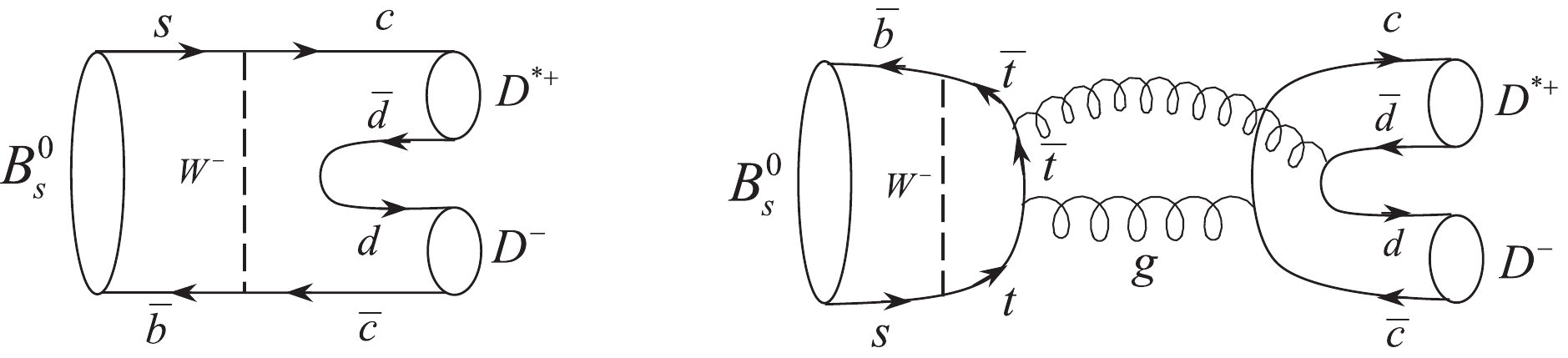
Figure 1. W-exchange and penguin-annihilation diagrams contributing to
$ B^0_s\rightarrow D^{*+}D^- $ decay.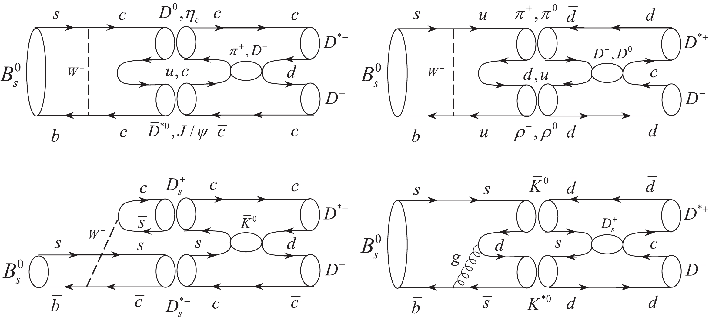
Figure 2. Intermediate state rescattering of
$ B^0_s\rightarrow P_1(p_1)P_2(p_2,\epsilon_2) \rightarrow D^{*+}(p_3,\epsilon_3)D^-(p_4) $ .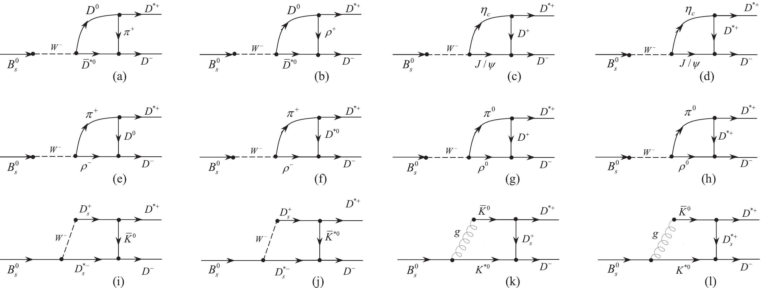
Figure 3. Hadronic loop level diagrams for long distance uncrossed t channel contribution to
$ B^0_s\rightarrow D^{*+}D^- $ decay.In these processes, the
$ \pi^+(\rho^+) $ ,$ D^+(D^{*+}) $ ,$ D^0(D^{*0}) $ ,$ D^+(D^{*+}) $ ,$ \bar{K}^0(\bar{K}^{*0}) $ , and$ D^+_s(D^{*+}_s) $ mesons are exchanged between the intermediate and final state mesons. The processes of producing these middle and exchanged particles are determined through Feynman diagrams. According to the final state interaction quark model, the Feynman graphs are presented in two channels: t and s. Unlike in D meson decays, in$ B_s $ meson decays there is no resonance with energy close to the mass of the$ B_s $ meson; consequently, the s channel is suppressed.The channel t occurs in both uncrossed and crossed ways. In uncrossed channels, two final mesons,
$ D^{*+} $ and$ D^- $ , share one quark and one anti-quark with the same flavor ($ d $ ). In this case, the intermediate mesons are produced by sharing$ u $ ,$ c $ , and$ s $ quarks (left graphs in the first and second rows in Fig. 2). If the intermediate mesons exchange a$ d $ quark, these mesons are identical to the final mesons, i.e.,$ B^0_s \rightarrow D^{*+}D^- \rightarrow D^{*+}D^- $ ; therefore, this mode is ignored.Moreover, in uncrossed channels, the
$ D^{*+} $ and$ D^- $ final mesons can share the$ c $ quark and$ \bar{c} $ anti-quark, respectively. In this case, the quarks that are shared between the final and middle mesons are$ d $ ,$ u $ , and$ s $ . The mode in which the middle mesons exchange quark$ c $ is ignored because a duplicate mode of$ B^0_s \rightarrow \bar{D}^{*0}\bar{D}^0 \rightarrow $ $ D^{*+}D^- $ is achieved.In crossed channels, two final mesons exchange
$ c $ (or$ d $ ) quark and$ \bar{c} $ (or$ \bar{d} $ ) anti-quark with intermediate mesons crosswise. Thus, the$ B^0_s \rightarrow D^{*+}D^- \rightarrow D^{*+}D^- $ process cannot take place. Twelve final state interaction diagrams in an uncrossed t channel are shown in Fig. 3.In factorization approaches, the perturbative strong phases arising from the penguin graph in
$ b\rightarrow s(d) $ transitions and from the vertex corrections can be in principle sizable. Modeling approaches based on final state interactions are soft rescattering processes. They are calculated through the nonperturbative theory. Therefore, the nonperturbative strong phases induced from power suppressed contributions should be considered. The idea that Hai-Yang Cheng reported about the existence of strong phases in final state interactions is that in charmless$ B $ decays, when the intermediate state mesons are charm, the elements of the CKM matrix of these states are dominant, and then, the absorptive part of the final state rescattering amplitude can cause large phases. However, if the final mesons are also charm (which is the case of the current study), the phases cannot have a significant contribution in the rates [6]. An interesting estimate on the basis of the Regge theory is provided by Donoghue et al. with this content: final state interactions appear even in the heavy quark limit and soft FSI phases are dominated by inelastic scattering [7]. However, it was later pointed out by Beneke et al. within the framework of QCD factorization that the above conclusion holds only for individual rescattering amplitudes. When summing over all possible intermediate states, there exist systematic cancellations in the heavy quark limit such that the strong phases must vanish in the limit$ m_b\rightarrow \infty $ [8]. -
Under the factorization approaches (Fa), the
$ B^0_s\rightarrow $ $ D^{*+}D^- $ decay occurs only through annihilation processes. These contributions to the matrix elements of the effective weak Hamiltonian can be written in the form [9]$ \langle D^{*+}D^-|\mathcal{H}_{\rm eff}|B^0_s \rangle = {\rm i}\frac{G_F}{\sqrt{2}}\lambda\langle D^{*+}D^-|\mathcal{T}^{\rm ann}|B^0_s \rangle, $

(3) where
$ \lambda $ is equal to$ V^*_{cb}V_{cs} $ and$ V^*_{tb}V_{ts} $ for the current-current tree and penguin level diagrams, respectively. The term$\mathcal{T}^{\rm ann}$ arises from weak annihilation contributions and the matrix elements of$\langle D^{*+}D^-|\mathcal{T}^{\rm ann}|B^0_s \rangle$ represent the$ b_i(D^*D) $ coefficients multiplied by the$ f_{B_s} $ ,$ f_{D^*} $ , and$ f_{D} $ decay constants. According to Fig. 1, the$ B^0_s\rightarrow D^{*+}D^- $ decay includes current-current annihilation$ (b_1(D^*D)) $ , penguin annihilation$ (b_4(D^*D)) $ , and electroweak penguin annihilation$(b_{4,\rm EW}(D^*D))$ coefficients, so the amplitude of this decay mode is obtained as follows:$\begin{aligned}[b] \mathcal{A}(B^0_s\rightarrow D^{+*}D^-)_{\rm fa} =& {\rm i}\frac{G_{F}}{\sqrt{2}}f_{B_s}f_{D^*}f_{D}\Bigg\{b_{1}V^*_{cb}V_{cs}\\&-\left(2b_4+\frac{1}{2}b_{4,\rm EW}\right)V^*_{tb}V_{ts}\Bigg\}, \end{aligned} $

(4) where the quantities
$ b_1 $ ,$ b_4 $ , and$b_{4,\rm EW}$ depend on the final-state mesons through the light-cone distribution amplitudes entering the expressions for$ A_{1,2}^i $ as [9]$\begin{aligned}[b]& b_{1} = \frac{C_{F}}{N_{c}^{2}}c_{1}A_{1}^{i},\quad b_{4} = \frac{C_{F}}{N_{c}^{2}}(c_{4}A_{1}^{i}+c_{6}A_{2}^{i}),\\& b_{4,\rm EW} = \frac{C_{F}}{N_{c}^{2}}(c_{10}A_{1}^{i}+c_{8}A_{2}^{i}), \end{aligned} $

(5) here
$ c_i $ denotes the Wilson coefficients,$ N_c $ is the color number, and$ C_F = (N_c^2-1)/(2N_c) $ . By considering a generic$ b $ -quark decay in the$ B_s\rightarrow M_1M_2 $ process, and using the convention that$ M_2 $ contains a quark and$ M_1 $ contains an antiquark from the weak vertices, it can be found that the type is$ B_s\rightarrow PV $ (Fig. 1 shows that the$ D^- $ meson has an antiquark and the$ D^{*+} $ meson has a quark, so they are considered as the pseudoscalar ($ P $ )$ M_1 $ and vector ($ V $ )$ M_2 $ mesons, respectively). For such a case, the basic building blocks of$ A_{1,2}^i $ are given by [9]$ \begin{aligned}[b]A_1^i =& 6\pi\alpha_s\int_0^1{\rm d}x{\rm d}y\Bigg\{6xy\bar{x}\bar{y}\Bigg[\frac{1}{y(1-x\bar{y})}+\frac{1}{\bar{x}^2y}\Bigg]+r_{\chi}^{D^*}r_{\chi}^{D} \frac{x-\bar{x}}{\bar{x}y}\Bigg\},\\ A_2^i =& -6\pi\alpha_s\int_0^1{\rm d}x{\rm d}y\Bigg\{6xy\bar{x}\bar{y}\Bigg[\frac{1}{\bar{x}(1-x\bar{y})} +\frac{1}{\bar{x}y^2}\Bigg]+r_{\chi}^{D^*}r_{\chi}^{D} \frac{x-\bar{x}}{\bar{x}y}\Bigg\}. \end{aligned}$

(6) In the above integrals, there are divergences for each of the final mesons: for the
$ D^- $ pseudoscalar meson, these divergences are$\int_0^1{\rm d}y/y$ and$\int_0^1 {\ln(y)}{\rm d}y/y$ , which are introduced with parameters$ X_A^D $ and$ -1/2(X_A^D)^2 $ , respectively, and similarly for the vector meson of$ D^{*+} $ with$ y\rightarrow \bar{x} $ . In general,$ X_A $ is allowed for three cases, namely$ PP $ ,$ PV $ , and$ VP $ . These values are modeled by using the parameterization [9]$ X_{A} = (1+\rho {\rm e}^{{\rm i}\phi})\ln{\frac{m_{B_s}}{\Lambda_h}}. $

(7) The quantity
$ \phi $ is an arbitrary strong-interaction phase that may be caused by soft rescattering. The values selected by Beneke and Neubert in Ref. [9] for the three cases, i.e.,$ PP $ ,$ PV $ , and$ VP $ are$ \phi = -55^\circ $ ($ PP $ ),$ \phi = -20^\circ $ ($ PV $ ), and$ \phi = -70^\circ $ ($ VP $ ), respectively. From the above discussion, it follows that because the final mesons are of$ PV $ type; thus, the value of$ \phi $ was set to$ -20^\circ $ . These authors also evaluated the Wilson coefficients$ b_i $ at an intermediate scale$\mu_h\sim(\Lambda_{\rm QCD}m_b)^{1/2}$ rather than$ \mu_h\sim m_b $ . Specifically, they used$ \mu_h = (\Lambda_h\mu)^{1/2} $ with$ \Lambda_h = 0.5 $ Gev. The value of the model parameter$ \rho $ is limited to$ \rho\leqslant 1 $ , so it was set as$ \rho = 0.5 $ in this study.Simple expressions can be obtained for
$ A_1^i $ and$ A_2^i $ [9]:$ A_{1}^{i}\approx -A_{2}^{i} = 6\pi\alpha_{s}\left[3\left(X_A-4+\frac{\pi^{2}}{3}\right)+r_{\chi}^{D^*}r_{\chi}^{D}(X_A^2-2X_A)\right]. $

(8) The light-cone expansion implies that only leading-twist distribution amplitudes are needed in the heavy-quark limit. There exist however a number of subleading quark-antiquark distribution amplitudes of twist 3 that have large normalization factors for pseudoscalar and vector mesons. For
$ D $ and$ D^* $ mesons, the ratios$ r_\chi^D $ and$ r_\chi^{D^*} $ are defined as [9]$ r_\chi^{D} = \frac{2m_D^2}{(m_b-m_c)(m_c+m_d)},\quad r_\chi^{D^*} = \frac{2m_D^*}{m_b}\frac{f_{D^*}^\perp}{f_{D^*}}.$

(9) For the running coupling constant, at two loop order (NLO), the solution of the renormalizaton group equation can always be written in the form
$ \alpha_s = \frac{4\pi}{\beta_{0}\mathrm{ln}\dfrac{\mu^2}{\Lambda_{\rm QCD}^2}}\left[1-\frac{\beta_1}{\beta_{0}^2} \frac{\mathrm{ln}\left(\mathrm{ln}\dfrac{\mu^2}{\Lambda_{\rm QCD}^2}\right)}{\mathrm{ln}\dfrac{\mu^2}{\Lambda_{\rm QCD}^2}}\right], $

(10) where
$ \beta_0 = (11N_c-2n_f)/3 $ ,$\beta_1 = (34N_c^2-10N_cn_f)/ $ $ 3-2C_Fn_f$ . In this study, the running$ \alpha_s(\mu) $ is evaluated with$ n_f = 5 $ .In the
$ B^0_s\rightarrow D^{*+}D^- $ decay, there is also the possibility of intermediate state rescattering, which greatly contributes to the calculation. Possible decays for the intermediate states derived from Feynman diagrams are shown in Fig. 4. Therefore, the amplitudes of the middle state decays used in the final state interactions are given by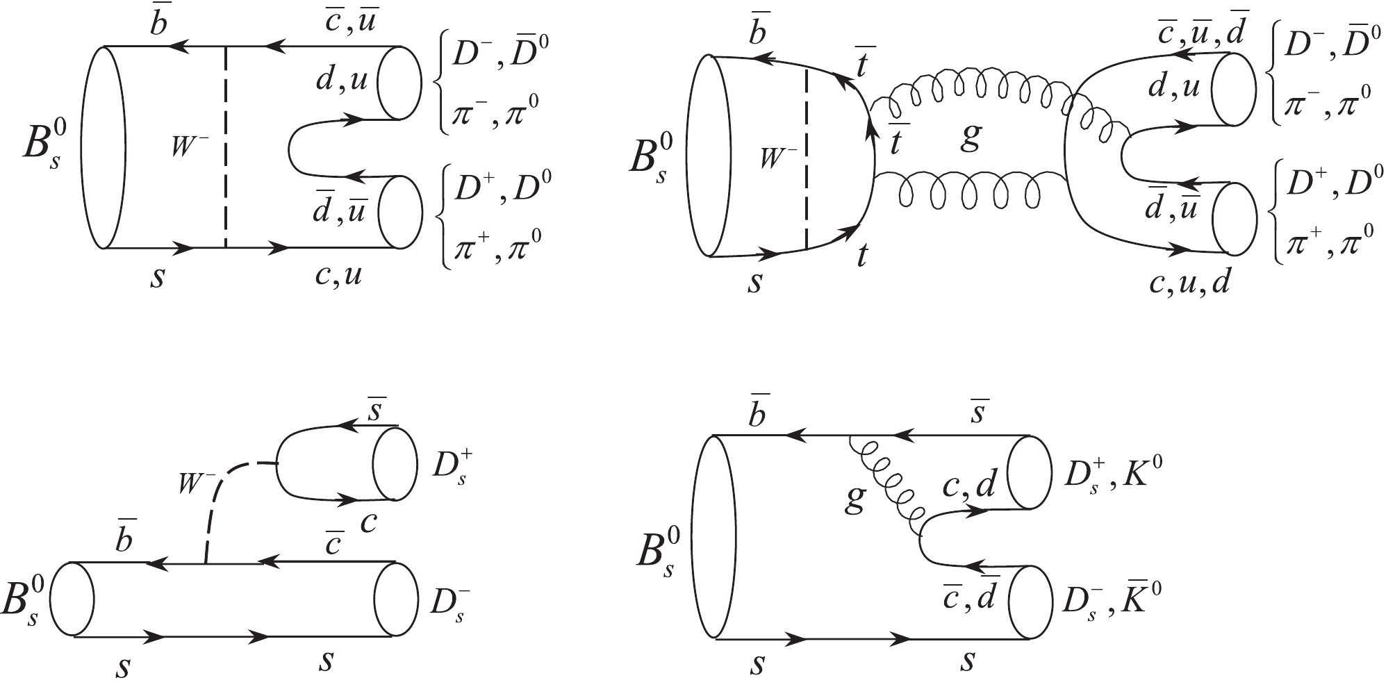
Figure 4.
$ B_s $ meson decay diagrams to intermediate state mesons in a rescattering process.$ \begin{aligned}[b] \mathcal{A}(B^0_s\rightarrow D^0\bar{D}^{*0}(\eta_cJ/\psi)) =& {\rm i}\frac{G_{F}}{\sqrt{2}}f_{B_s}f_{D}f_{D^*}(f_{\eta_c}f_{J/\psi}) [b_{1}V^*_{cb}V_{cs}\\&-(2b_4+2b_{4,\rm EW})V^*_{tb}V_{ts}],\\ \mathcal{A}(B^0_s\rightarrow \pi^+\rho^-) =& {\rm i}\frac{G_{F}}{\sqrt{2}}f_{B_s}f_{\pi}f_{\rho} [b_{1}V^*_{ub}V_{us}\\&-\left(2b_4+\frac{1}{2}b_{4,EW}\right)V^*_{tb}V_{ts}],\\ \mathcal{A}(B^0_s\rightarrow \pi^0\rho^0) =& {\rm i}\frac{G_{F}}{2}f_{B_s}f_{\pi}f_{\rho}b_{1}V^*_{ub}V_{us},\\ \mathcal{A}(B^0_s\rightarrow D^+_sD^{*-}_s) =& {\rm i}\sqrt{2}G_F m_{D_s^*}(\epsilon_{D_s^*}.p_{B_s}) f_{D_s} A_0^{B_s\rightarrow D_s^*}\\&\times(m_{D_s}^2)(a_1V^*_{cb}V_{cs}-a_4V^*_{tb}V_{ts}),\\ \mathcal{A}(B^0_s\rightarrow \bar{K}^0K^{*0}) =& -{\rm i}\sqrt{2}G_F m_{K^*}(\epsilon_{K^*}.p_{B_s})\\&\times f_{K}A_0^{B_s\rightarrow K^*}(m_{K}^2)a_4V^*_{tb}V_{ts}. \end{aligned}$

(11) -
Diagram (3a) in Fig. 3 shows the absorptive part of the amplitude for the
$ B^0_s\rightarrow D^0(p_1)\bar{D}^{*0}(\epsilon_2,p_2)\rightarrow D^{*+}(\epsilon_3,p_3) $ $ D^-(p_4) $ mode in the t channel one particle exchange process. In this process, intermediate state decay occurs by the annihilation topology and the exchanged meson is$ \pi^+ $ , so the absorptive part of the amplitude is given by$\begin{aligned}[b] \mathcal{A}bs^{3a} =& \frac{g_{D^*D\pi}^2}{8\pi m_{B_s}}\mathcal{A}(B^0_s\rightarrow D^0\bar{D}^{*0})\\&\times\int_{-1}^{1}|\vec{p_{1}}|d(\cos\theta)\frac{F^{2}(q^{2},m_{i}^{2})}{\mathcal{T}^{3a}}\mathcal{H}^{3a},\end{aligned} $

(12) where
$ \theta $ is the angle between$ \vec{p_{1}} $ and$ \vec{p_{3}} $ for which$ p_1 $ and$ p_3 $ are the four-momentums of the$ D^0 $ and$ D^{*+} $ mesons, q and$ m_{i} $ are the momentum and mass of the exchange$ \pi^+ $ meson, respectively, and$ \begin{aligned}[b] \mathcal{H}^{3a} =& (\epsilon_3.p_1)(\epsilon_2.p_4) \\=& \left(\frac{E_1|\vec{p_3}|-E_3|\vec{p_1}|\cos\theta}{m_{B_s}|\vec{p_3}|}\right) \left(\frac{E_4|\vec{p_2}|-E_2|\vec{p_4}|\cos\theta}{m_{B_s}|\vec{p_2}|}\right),\\ \mathcal{T}^{3a} =& (p_1-p_3)^{3}-m_\pi^{2} \\=& p_1^2+p_3^2-2p_1^0p_3^0+2p_1.p_2-m_\pi^2\\ =& m_D^{2}+m_{D^*}^{2}-m_\pi^{2}-2E_DE_{D^*}+2|\vec{p}_{D}||\vec{p}_{D^*}|\cos\theta. \end{aligned} $

(13) Note that
$ F(q^{2},m_{i}^{2}) $ is the form factor defined to account for the off-shell character of the exchange particles, defined as$ (\Lambda^{2}-m_{i}^{2})/(\Lambda^{2}-q^{2}) $ [10]. Concerning$ \Lambda $ , it is a phenomenological parameter that should not be far from the physical parameters of the exchange particle,$ m_{i} $ and q; it can be written in terms of another phenomenological parameter, for instance,$ \eta $ , as$\Lambda = m_{i}+\eta\Lambda_{\rm QCD}$ . The range of the strong interaction energy scale,$\Lambda_{\rm QCD}$ , goes from$ (90.6\pm3.4 $ ) MeV to$ (340\pm8) $ MeV [11]. We set it as$\Lambda_{\rm QCD} = 225$ MeV. The numerical value of the branching ratio in the final state interaction is very sensitive to the$ \eta $ parameter. According to the exchanged mesons, variable values ranging from 0.5 to 5 can be found. In Ref. [10], the exchanged mesons are$ D $ and$ D^* $ , so the authors set$ \eta = 0.5-3.0 $ . However, the authors of Ref. [12], with the same exchanged mesons, set$ \eta\sim 5 $ . In this regard, in [13], a value of 4 was set for this phenomenological parameter. On the other hand, in Ref. [14], the value of$ \eta $ was selected according to the mass of the meson exchanged:$ \eta = 2.2 $ for the exchanged particle$ D^* $ (or$ D $ ) and$ \eta = 1.1 $ for$ \rho $ (or$ \pi $ ). In the present study, given that the exchanged mesons are$ D^{(*)}_{(s)} $ ,$ \pi(\rho) $ , and$ K^{(*)} $ , to select the values of$ \eta $ , Ref. [14] was followed. Similarly, for diagram (3b), in which the decay of the intermediate state also occurs by the annihilation topology, the absorptive part of the amplitude can be written as$\begin{aligned}[b] \mathcal{A}bs^{3b} =& \frac{g^2_{D^*D\rho}}{8\pi m_{B_s}}\mathcal{A}(B^0_s\rightarrow D^0\bar{D}^{*0}) \\&\times\int_{-1}^{1}|\vec{p_{1}}|d(\cos\theta)\frac{F^{2}(q^{2},m_\rho^2)}{\mathcal{T}^{3b}}\mathcal{H}^{3b}, \end{aligned}$

(14) where
$ \begin{aligned}[b] \mathcal{H}^{3b} =& \epsilon_{\mu\nu\alpha\beta}\epsilon_{\rho\sigma\lambda\eta}\epsilon_\rho^{\nu}\epsilon_\rho^{\sigma} \epsilon_{3}^{\mu}\epsilon_{2}^{\rho}p_{1}^{\alpha}p_3^{\beta}p_2^{\lambda} p_{4}^{\eta},\\ \mathcal{T}^{3b} =& m_D^{2}+m_{D^*}^{2}-m_\rho^{2}-2E_DE_{D^*}+2|\vec{p}_D||\vec{p}_{D^*}|\cos\theta. \end{aligned} $

(15) -
The absorptive part of the amplitude for the
$B^0_s\rightarrow \eta_c(p_1)\times J/\psi(\epsilon_2,p_2)\rightarrow D^{*+}(\epsilon_3,p_3) D^-(p_4)$ mode with$ D^+ $ and$ D^{*+} $ exchanged mesons is obtained as follows (the intermediate state of this process is also based on the annihilation topology):$ \begin{aligned}[b] \mathcal{A}bs^{3c(3d)} =& \frac{g_{D^*D^{(*)}\eta_c}g_{J/\psi D^{(*)}D}}{8\pi m_{B_s}}\mathcal{A}(B^0_s\rightarrow \eta_cJ/\psi)\\&\times\int_{-1}^{1}|\vec{p_{1}}|d(\cos\theta)\frac{F^{2}(q^{2},m_{D(D^*)}^{2})}{\mathcal{T}^{3c(3d)}}\mathcal{H}^{3a(3d)},\end{aligned}$

(16) where
$ \begin{aligned}[b] \mathcal{T}^{3c} =& m_{\eta_c}^{2}+m_{D^*}^{2}-m_D^{2}-2E_{\eta_c}E_{D^*}+2|\vec{p}_{\eta_c}||\vec{p}_{D^*}|\cos\theta,\\ \mathcal{H}^{3d} =& \epsilon_{\mu\nu\alpha\beta}\epsilon_{\rho\sigma\lambda\eta}\epsilon_{D^*}^{\nu}\epsilon_{D^*}^{\sigma} \epsilon_{3}^{\mu}\epsilon_{2}^{\rho}p_{1}^{\alpha}p_3^{\beta}p_2^{\lambda} p_{4}^{\eta},\\ \mathcal{T}^{3d} =& m_{\eta_c}^{2}-2E_{\eta_c}E_{D^*}+2|\vec{p}_{\eta_c}||\vec{p}_{D^*}|\cos\theta. \end{aligned} $

(17) -
The intermediate state decays
$B^0_s\rightarrow \pi^+(p_1)\times $ $ \rho^-(\epsilon_2,p_2)$ and$ B^0_s\rightarrow \pi^0(p_1)\rho^0(\epsilon_2,p_2) $ are also transformed into final mesons through processes of annihilation. The absorptive part of the amplitudes for these decay modes are calculated by$ \begin{aligned}[b] \mathcal{A}bs^{3e(3f)} =& \frac{g_{D^*D^{(*)}\pi}g_{D D^{(*)}\rho}}{8\pi m_{B_s}}\mathcal{A}(B^0_s\rightarrow \pi^+\rho^-)\\&\times\int_{-1}^{1}|\vec{p_{1}}|d(\cos\theta)\frac{F^{2}(q^{2},m_{D(D^*)}^{2})}{\mathcal{T}^{3e(3f)}}\mathcal{H}^{3a(3d)}, \end{aligned}$

(18) where
$ \begin{aligned}[b] \mathcal{T}^{3e} =& m_\pi^{2}+m_{D^*}^{2}-m_D^{2}-2E_\pi E_{D^*}+2|\vec{p}_\pi||\vec{p}_{D^*}|\cos\theta,\\ \mathcal{T}^{3f} =& m_\pi^{2}-2E_\pi E_{D^*}+2|\vec{p}_\pi||\vec{p}_{D^*}|\cos\theta. \end{aligned} $

(19) Graphs (3g) and (3h) in Fig. 3 were also calculated for the
$ B^0_s\rightarrow \pi^0(p_1)\rho^0(\epsilon_2,p_2)\rightarrow D^{*+}(\epsilon_3,p_3) D^-(p_4) $ mode using Eqs. (18) and (19), with the difference that the amplitude of$ \mathcal{A}(B^0_s\rightarrow \pi^0\rho^0) $ was replaced by$ \mathcal{A}(B^0_s\rightarrow \pi^+\rho^-) $ . -
The
$ B^0_s\rightarrow D^+_s(p_1)D^{*-}_s(\epsilon_2,p_2) $ decay, which is considered to be another intermediate state decay, decays through a dominant tree and penguin contributions. The absorptive part of the amplitude for the mode of$ B^0_s\rightarrow D^+_s(p_1)D^{*-}_s(\epsilon_2,p_2)\rightarrow D^{*+}(\epsilon_3,p_3) D^-(p_4) $ can be obtained by$ \begin{aligned}[b] \mathcal{A}bs^{3i(3j)} =& {\rm i}\frac{G_{F}}{\sqrt{2} }\frac{g_{D^*D_sK^{(*)}}g_{D_s^*DK^{(*)}}}{4\pi m_{B_s}}\\&\times m_{D^*_s}f_{D_s}A_0^{B_s\rightarrow D^*_s}(m_{D_s}^2)(a_1V^*_{cb}V_{cs}+a_4V^*_{tb}V_{ts})\\ &\times\int_{-1}^{1}|\vec{p_{1}}|d(\cos\theta)\frac{F^{2}(q^{2},m_{K(K^*)}^{2})}{\mathcal{T}^{3i(3j)}}\mathcal{H}^{3i(3j)}, \end{aligned} $

(20) where
$ \begin{aligned}[b] \mathcal{H}^{3i} =& (\epsilon_2.p_1)(\epsilon_2.p_4)(\epsilon_3.p_1)\\ =& \left(-p_1.p_4+\frac{(p_1.p_2)(p_2.p_4)}{m^2_{D^*_s}}\right) \left(\frac{E_1|\vec{p_3}|-E_3|\vec{p_1}|\cos\theta}{m_{B_s}|\vec{p_3}|}\right),\\ \mathcal{H}^{3j} =& m_3^2(p_1.p_2)-(p_1.p_3)(p_2.p_3)\\&+\left(\frac{E_2|\vec{p_3}|-E_3|\vec{p_2}|\cos\theta} {m_{B_s}|\vec{p_3}|}\right)[(p_{B_s}.p_1)(p_3.p_4)\\&-(p_{B_s}.p_3)(p_1.p_4)],\\ \mathcal{T}^{3i(3j)} =& m_{D_s}^{2}+m_{D^*}^{2}-m_K^{2}(m_{K^*}^{2})\\&-2E_{D_s} E_{D^*}+2|\vec{p}_{D_s}||\vec{p}_{D^*}|\cos\theta. \end{aligned} $

(21) -
The last decay of the intermediate state under consideration, i.e., the decay of
$ B^0_s\rightarrow \bar{K}^0(p_1)K^{*0}(\epsilon_2,p_2) $ , occurs through a penguin contribution. Thus, the absorptive part of the amplitude reads$ \begin{aligned}[b] \mathcal{A}bs^{3k(3l)} =& {\rm i}\frac{G_{F}}{\sqrt{2} }\frac{g_{D^*D_s^{(*)}K}g_{D_s^{(*)}DK^*}}{4\pi m_{B_s}}\\&\times m_{K^*}f_KA_0^{B_s\rightarrow K^*}(m_K^2)a_4V^*_{tb}V_{ts}\\& \times\int_{-1}^{1}|\vec{p_{1}}|d(\cos\theta)\frac{F^{2}(q^{2},m_{D_s(D_s^*)}^{2})}{\mathcal{T}^{3k(3l)}}\mathcal{H}^{3k(3j)}, \end{aligned} $

(22) where
$ \mathcal{H}^{3k} $ is calculated following a procedure similar to that of$ \mathcal{H}^{3i} $ ; concerning$ \mathcal{H}^{3k} $ , the parameter$ m_{K^*}^2 $ was employed instead of$ m_{D^*_s}^2 $ , and$ \begin{aligned}[b] \mathcal{T}^{3k(3l)} =& m_K^{2}+m_{D^*}^{2}-m_{D_s}^{2}(m_{D_s^*}^{2})-2E_K E_{D^*}\\&+2|\vec{p}_K||\vec{p}_{D^*}|\cos\theta. \end{aligned}$

(23) -
The dispersive part of the intermediate state rescattering amplitudes can be obtained from the absorptive parts shown in Fig. 3 using the following dispersion relation [14,15]:
$ \begin{aligned}[b]& {\rm Dis}\mathcal{A}(m_{B_s}^2) = \frac{1}{\pi}\\&\times \int_{s}^{\infty}\frac{\mathcal{A}bs^{3a}(s')+\mathcal{A}bs^{3b}(s') +\mathcal{A}bs^{3c}(s')\ldots +\mathcal{A}bs^{3l}(s')}{s'-m_{B_s}^2}{\rm d}s'. \end{aligned}$

(24) where
$ s' $ is the square of the momentum carried by the exchanged particle and s is the threshold of intermediate states, in this case$ s\sim m_{B_s}^2 $ .The total amplitude of the absorptive and dispersive parts of the intermediate state rescattering (Isr) is estimated by
$\begin{aligned}[b] \mathcal{A}(B^0_s\rightarrow D^{*+}D^-)_{\rm Isr} =& {\rm i}\mathcal{A}bs^{3a}+{\rm i}\mathcal{A}bs^{3b}+\dots\\&+{\rm i}\mathcal{A}bs^{3l}+{\rm Dis}\mathcal{A}(m_{B_s}^2). \end{aligned} $

(25) -
The decay rate of
$ B^0_s\rightarrow D^{*+}D^- $ in$ B_s $ meson rest frame under the factorization approach can be written as [16]$ \Gamma(B^0_s\rightarrow D^{*+}D^-)_{\rm Fa} = \frac{1}{8\pi}\frac{|\vec{p}|}{m_{B_s}^2}|\mathcal{A}(B^0_s\rightarrow D^{*+}D^-)_{\rm Fa}|^2, $

(26) where
$ |\vec{p}| $ is the absolute value of the 3-momentum of the$ D^* $ or$ D $ final mesons, which can be calculated using$ \sqrt{(m_{B_s}^2+m_{D^*}^2-m_D^2)^2-4m_{B_s}^2m_{D^*}^2}/(2m_{B_s}) $ . The branching ratio of the$ B^0_s\rightarrow D^{*+}D^- $ decay using the factorization method is expressed as$ \mathcal{B}(B^0_s\rightarrow D^{*+}D^-)_{\rm Fa} = \frac{\Gamma(B^0_s\rightarrow D^{*+}D^-)_{\rm Fa}}{\Gamma_{\rm tot}},$

(27) where the value of
$\Gamma_{\rm tot}$ for the$ B_s $ meson is$ (4.34\pm0.01)\times10^{-13} $ GeV.Finally, the branching fraction of the
$ B^0_s\rightarrow D^{*+}D^- $ decay applying the factorization model while considering the effects of rescattering of intermediate states is given by$ \begin{aligned}[b] \mathcal{B}(B^0_s\rightarrow D^{*+}D^-)_{\rm Fa+Isr} =& \frac{1}{\Gamma_{\rm tot}}\frac{|\vec{p}|}{8\pi m_{B_s}^2}|\mathcal{A}(B^0_s\rightarrow D^{*+}D^-)_{\rm Fa}\\&+\mathcal{A}(B^0_s\rightarrow D^{*+}D^-)_{\rm Isr}|^2. \end{aligned}$

(28) -
The calculations of the branching fractions are provided next. The input parameters used in this paper are as follows:
$ \mathbf{masses\;and\;decay\;constants\;} $ (in units of MeV) [11]$\begin{aligned}[b]& m_{B^0_s} = 5366.88\pm0.14\quad m_{\eta_c} = 2983.9\pm0.5\\ & m_{D^*_s} = 2112.2\pm0.4 \quad m_{D^*} = 2006.85\pm0.05\\ & m_{D_s} = 1968.34\pm0.07 \quad m_D = 1869.65\pm0.05\\ & m_{K^*} = 891.66\pm0.26 \quad m_\rho = 775.26\pm0.25 \\ & m_K = 493.677\pm0.016 \quad m_\pi = 139.57039\pm0.00018 \\ & m_b = 4180\pm0.02 \quad m_c = 1270\pm20\\ & m_d = 4.69\pm0.32\quad f_{J/\psi} = 418\pm9 \quad f_{\eta_c} = 387\pm7 \\&f_{D^*} = 340\pm23\quad f_{D_s} = 294\pm7 \quad f_{B_s} = 245\pm25 \\&f_D = 234\pm15\quad f_{D^*}^\perp = 216\pm14 \quad f_\rho = 210\pm4\\ &f_K = 159.80\pm1.84\quad f_\pi = 130.70\pm0.46 \end{aligned} $

$ \mathbf{CKM\;matrix\;elements} $ [11]$ \begin{aligned}[b] &V_{cb} = (41.0\pm1.4)\times10^{-3} \quad V_{ub} = (3.82\pm0.24)\times10^{-3}\\& V_{ts} = (38.8\pm1.1)\times10^{-3} \quad V_{cs} = 0.987\pm0.011\\ & V_{us} = 0.2245\pm0.0008\quad V_{tb} = 1.013\pm0.030 \end{aligned} $

$ \mathbf{Wilson\;coefficients} $ $ (\mu = m_b,\;\alpha = 1/129) $ [17]$ \begin{aligned}[b] & c_1 = 1.081\quad c_4 = -0.036\quad c_6 = -0.042 \quad c_8/\alpha = 0.060\\& c_{10}/\alpha = 0.223 \end{aligned} $

$ \mathbf{coupling\;constants} $ [14,18,19,20]$ \begin{aligned}[b] &g_{J/\psi DD} = 7.71 \quad g_{J/\psi D^*D} = 8.64\quad g_{D^*D\pi} = 8.84\\ & g_{D^*D^*\pi} = 9.08 \quad g_{DD\rho} = 2.52 \quad g_{D^*D\rho} = 2.82\\ & g_{D^*D_sK} = 12.84 \quad g_{D^*D_sK^*} = 2.79 \quad g_{D_s^*DK^*} = 3.00\\ & g_{D_sDK^*} = 2.66 \quad g_{D^*_sDK} = 2.89 \quad g_{D^*D^*_sK} = 9.23\\& g_{D^*D\eta_c} = 8.52 \end{aligned} $

$ \mathbf{form\;factors} $ [21,22]$ A_0^{B_s\rightarrow K^*}(m_K^2) = 0.306\pm0.034 \quad A_0^{B_s\rightarrow D^*_s}(m_{D_s}^2) = 0.883\pm0.012 . $

Finally, the branching fractions for the
$ B^0_s\rightarrow D^{*+}D^- $ decay under the factorization approach and applying the factorization method while considering rescattering of the final state interaction read, respectively, as follows:$ \mathcal{B}(B^0_s\rightarrow D^{*+}D^-)_{\rm Fa} = (2.41\pm1.37)\times10^{-5}, $

(29) and
$ \mathcal{B}(B^0_s\rightarrow D^{*+}D^-)_{\rm Fa+Isr} = (8.27\pm2.23)\times10^{-5}. $

(30) There are some parameters in the hadronic decays that can be obtained from theoretical estimates, such as transition form factors. In practice, information about form factors often comes from theoretical calculations such as light-cone QCD sum rules or lattice calculations. Thus, they usually present large uncertainties. In this framework, the theoretical uncertainties expressed in Eqs. (29) and (30) arise from the uncertainties in the form factors, CKM matrix elements, decay constant, meson messes, and total decay rate of
$ B_s $ meson. The corresponding uncertainties in the form factors and CKM matrix elements have more impact on the results. -
In this study, the contribution of the uncrossed t channel final state interaction, i.e., inelastic re-scattering processes to the branching ratio of
$ B^0_s\rightarrow D^{*+}D^- $ decay, is calculated. For evaluating these effects, the absorptive and dispersive parts of the hadronic loop level diagrams were considered because the hadrons produced via weak interaction were on their mass shells.The branching ratio of the
$ B^0_s\rightarrow D^{*+}D^- $ decay was obtained through the factorization approach and final state interaction. The experimental result of this decay is$ \mathcal{B}(B^0_s\rightarrow D^{*+}D^-) = (8.41\pm1.02)\times 10^{-5} $ . The branching ratios of this decay reported in Refs. [4,5] were$ (6.1\pm3.6)\times10^{-5} $ and a much larger value,$ (3.6\pm0.6)\times10^{-3} $ , respectively. According to the factorization approach and considering the effects of final state interaction as an effective correction, the obtained results are$ \mathcal{B}(B^0_s\rightarrow D^{*+}D^-) = (2.41\pm1.37)\times10^{-5} $ and$ \mathcal{B}(B^0_s\rightarrow D^{*+}D^-) = (8.27\pm2.23)\times10^{-5} $ , respectively.There are some phenomenological parameters such as
$ \eta $ in the calculations on final state interaction effects and in the form factors of the hadronic loop level diagrams. The value of the phenomenological parameter$ \eta $ in the form factor is expected to be of the order of unity and can be determined from the measured rates. For a given exchanged particle,$ \eta = 2.2 $ was set for the exchanged particles$ D^*_{(s)} $ (or$ D_{(s)} $ ) and$ \eta = 1.1 $ for$ \rho $ ,$ K^* $ (or$ \pi $ ,$ K $ ).
Pure annihilation decay of strange beauty meson into two charm heavy mesons
- Received Date: 2021-09-13
- Available Online: 2022-02-15
Abstract: In this study, the heavy to heavy decay of


 DownLoad: