


 Abstract
 HTML
HTML Reference
 Related
 PDF
PDF


-
In a non-central heavy-ion collision (HIC), a large vorticity and strong magnetic field are expected to be generated in extremely hot quark gluon plasma (QGP). Straightforward electromagnetic (EM) computation reveals that the magnetic field would reach approximately
$ O(10^{14})T $ [1] in the early stage of a HIC, while kinetic and hydrodynamic simulations [2,3] indicate that the local vorticity would exceed$0.5\;{\rm fm}^{-1}$ with the total angular momentum of QGP in the range of$ O(10^{4})-O(10^{5})\hbar $ . Known as the Barnett and magnetization effects, spin particles are polarized by these pseudo vector fields; thus, their distributions differ from normal thermal distributions. Besides the chiral effects induced by such pseudo vector fields [4-6], studies on these distribution modifications are useful to understand the hadronization mechanism of the strong interaction. Inspired by the large amplitude and retention owing to angular momentum conservation, vorticity has recently attracted more attention.Compared with magnetic field effects, rotation-related effects are electric charge blind and only involve the kinetic properties of QGP and the strong interaction; these are the aspects we are most interested in. Experimentally, to screen out EM effects, neutral particles with finite spin numbers are chosen as carriers of vorticity polarization effects. As it is difficult to directly detect an uncharged particle, the distribution of its charged daughter particle serves as an alternative observable for the global polarization effect. With the help of the Λ meson, the average magnitude of the vorticity of QGP was extracted by the STAR collaboration [7]. In these measurements, the expectation of Λ polarization and the vorticity behavior of the collision energy were confirmed. The results may be understood by considering the energy shift induced by the vorticity polarization to the spins; however, this theory becomes slightly vague when the
$ K^{*0} $ and ϕ meson measurements, presented in [8], are considered. The mismatch between these measurements indicates that the fine structure of hadrons may play a non-negligible role in polarization processes.The mass is one of the most fundamental attributes of a hadron. For a composite particle, the mass is modified by the single-particle dispersion relation of the fundamental degree of freedom as well as its interactions. Studies of hadron masses enable us to discover many clues regarding the environment from which hadrons originate. As a well-known example,
$ \sigma $ meson and pion masses change with increasing temperature and chemical potential because of chiral restoration [9]. Recently, the mass of the vector meson ρ in an external magnetic field has been studied while taking into account the polarization effect on quarks. A lattice calculation demonstrated that a charged ρ meson mass first decreases and then increases, with a minimum of approximately$eB\simeq $ $ 1 \; {\rm GeV}^{2}$ [10]. Using effective models such as the Nambu–Jona-Lasinio (NJL) model with a vector channel, the ρ meson with different spin components has been studied [11,12]. As a result, the mass behavior in a background vorticity field, which initially appears to be similar to the magnetic case, is brought into question. For the rotating effect, the co-rotating frame [13] is usually adopted and a nontrivial spin connection term is introduced [14], which serves as a polarization term for angular momentum. With this extended NJL model, chiral phase transition may occur as angular velocity increases [15]. Additionally, more complicated phase diagrams that combine rotation and other physical conditions, such as chemical potential, isospin and magnetic fields [16-18], have been established. In those NJL models, the rotation always behaves as an effective chemical potential at the quark level. This analogy has been explained with a Hamiltonian shift of$ \hat{H}\rightarrow \hat{H}-\vec{\omega}\cdot\hat{J} $ , where the latter term may correspond to an effective chemical potential [18,19]. At the same quark level, holographic models also expand upon our understanding of rotating quark matter by using a four-dimensional AdS-Kerr-Newman black hole to construct a rotation-magnetism analogy [20]. However, for composite hadrons, such as vector mesons, there have been few studies on their mass behaviors.In this paper, we focus on scalar and vector mesons and investigate their masses under rotation at a finite chemical potential. To consider both the finite temperature and density cases, we introduce the two-flavor NJL model with a vector channel in the co-rotating frame in Sec. II. With this framework, we generate a dynamical quark mass with spontaneous chiral symmetry breaking and construct scalar and vector mesons with the dressed quark propagator, while extracting the corresponding masses using the random phase approximation (RPA), in Sec. III; the numerical results are presented in Sec. IV. Owing to the rich phase structure at large chemical potentials, only
$ \mu_q $ < 200 MeV is investigated in this study and discussions on rotating color superconductivity are reserved for future studies. We discovered that scalar meson masses are controlled by chiral phase transition, which can be driven by temperature, density, and rotation. In contrast, vector mesons, which carry the net angular momentum, are governed by the polarization effect on the total angular momentum before chiral symmetry restoration. At large angular velocities, the mass of the spin component$ s_z = 1 $ of the vector meson vanishes. This indicates the macroscopic condensate of the spin component$ s_z = 1 $ of the vector meson$ \langle \rho^{s_z = 1}\rangle $ ; thus, spontaneous spin polarization would be induced in the ultra-fast rotating system. In Sec. V, we summarize our main results and provide an outlook. -
The NJL model is an effective model with a four-fermion interaction, which is widely used to study quark-quark and quark-antiquark pairings that correspond to chiral phase transition, superfluidity, and superconductivity. Besides the usual scalar channels, we consider vector channels to construct vector ρ mesons. The Lagrangian of the two-flavor NJL model in a co-rotating frame is given by [16,21]
$ \begin{aligned}[b]\mathcal{L} =& \bar{\psi}[{\rm i}\bar{\gamma}^{\mu}(\partial_{\mu}+\Gamma_{\mu})-m]\psi+G_S[(\bar{\psi}\psi)^2+(\bar{\psi}{\rm i}\gamma_5\vec{\tau}\psi)^2]\\&-G_V[(\bar{\psi}\gamma_{\mu}\psi)^2+(\bar{\psi}\gamma_{\mu}\gamma_5\psi)^2],\end{aligned} $

(1) where m is the current quark mass, and
$ G_{S} $ and$ G_{V} $ are the coupling constants in the scalar and vector channels, respectively. In a curved co-rotating frame, the gamma matrices$ \bar{\gamma}^{\mu} $ should be defined according to the corresponding Clifford algebra. The curved gamma matrices are related to their flat counterparts using the vierbein as$ \bar{\gamma}^{\mu} = e_{a}^{\ \mu}\gamma^{a} $ in which$ e_{a}^{\ \mu} $ should satisfy$ g_{\mu\nu} = \eta_{ab}e^{a}_{\ \mu}e^{b}_{\ \nu} $ , where$ \eta_{ab} $ is the metric of flat space-time and$ \gamma^{a} $ represents the flat gamma matrices. In our case, a simple choice is$ e^{a}_{\ \mu} = \delta^a_{\ \mu}+ \delta^a_{\ i}\delta^0_{\ \mu} \, v_i $ and$ e_{a}^{\ \mu} = \delta_a^{\ \mu} - \delta_a^{\ 0}\delta_i^{\ \mu} \, v_i $ , where$ v_i $ is the linear velocity$ \vec{v} = \vec{\omega}\times\vec{x} $ in the presence of a constant angular velocity$ \vec{\omega} $ . The spinor connection is given by$ \Gamma_\mu = \dfrac{1}{4}\times\dfrac{1}{2}[\gamma^a,\gamma ^b] \, \Gamma_{ab\mu} $ , where$ \Gamma_{ab\mu} = \eta_{ac}(e^c_{\ \sigma} G^\sigma_{\ \mu\nu}e_b^{\ \nu}- $ $ e_b^{\ \nu}\partial_\mu e^c_{\ \nu}) $ , and$ G^\sigma_{\ \mu\nu} $ is the general Christoffel connection determined by$ g_{\mu\nu} $ [13-15]. Within the slow velocity limit$ |\vec{\omega}\times\vec{x}|\ll c $ , only the$ O(\vec{v}) $ terms can be retained, which are reduced to the ordinary polarization form$ \vec{\omega}\cdot\vec{J} $ , where$ \vec{J} = \vec{x}\times\vec{p}+\vec{S} $ is the total angular momentum [14,15], and$ \vec{S} = \dfrac{1}{2}\left( \begin{array}{cc} \vec{\sigma} & 0 \\ 0 & \vec{\sigma} \\ \end{array} \right) $ is the spin operator.By applying the mean field approximation and choosing the direction of rotation to be the z-axis, the bilinear part of the Lagrangian at a finite chemical potential is given by [16]
$ \mathcal{L} = \bar{\psi}[{\rm i}\gamma^{\mu}\partial_{\mu}+\gamma^{0}(\omega \hat{J_{z}}+\mu)-M]\psi-\frac{(M-m)^{2}}{4G_{S}}, $

(2) where
$ J_{z} $ is the third component of the total angular momentum$ \vec{J} $ , and μ is the quark chemical potential. The angular velocity plays a similar role to the chemical potential, and M is the constituent quark mass, which is given by the chiral condensate using$M = m - $ $ 2G_S\left < \bar\psi\psi\right >$ .Quantum field theory for a rotating system was established by Vilenkin in [22], in which the Green function without the boundary condition was introduced. However, it was emphasized that a rotating system cannot have a radius R size larger than
$ \omega^{-1} $ , which is constrained by causality with the angular velocity ω and the radius of the system R. In this study, we apply an explicit form of the propagator in [22]. In realistic heavy-ion collisions, the average global velocity$ \langle\omega\rangle $ of QGP generally requires approximately 20 MeV [3,23], which should be safe when using an infinite size approximation. When considering the local vorticity, as shown in [3], the boundary conditions would become more important for a small vorticity lattice with a high angular velocity. In general, one should consider the inhomogeneity of the rotating fluid and solve M as r-dependent while considering the boundary conditions, as investigated in Refs. [24-34]. It was observed in [24] that M is almost constant except in the vicinity of the boundary. Furthermore, the bounded rotating system was studied self-consistently in [25], that is, beyond the local potential approximation. It is shown that the chiral condensate suppression effect is qualitatively unchanged by the boundary conditions and are quantitatively comparable in the bounded and boundless cases at finite temperatures. From a realistic point of view, boundary conditions always have effects in the near-surface part of QGP, and chiral condensation will not be significantly affected in the inner part of QGP. Instead of fully considering the inhomogeneous rotation and subtle boundary conditions, we choose a simplified scheme as the first step of this study to introduce the$ M(\omega) $ qualitative relation, which is easily estimated by noting the energy shifts of quarks owing to the polarization effects induced by rotation. We reserve the more self-consistent treatment of$ M(\omega) $ for future studies.In this study, we aim to investigate meson properties under rotation. To perform calculations in the NJL model, a
$ M(\omega) $ relation is required; hence,$ M(\omega) $ is extracted from the general grand potential given by [15,16]$ \begin{aligned}[b] \\[-8pt] \Omega(T,\mu,M,\omega) = &\int {\rm d}^3 \mathbf{r}\; \Bigg\{\frac{(M-m)^2}{4G_S} -\frac{N_c N_f}{16\pi^2} T \sum_n\int {\rm d} k_t^2 \int {\rm d} k_z[J_n(k_t r)^2+J_{n+1}(k_t r)^2]\left[ \ln(1+{\rm e}^{(E_k-(n+\frac{1}{2})\omega-\mu)/T})\right. \\& + \left. \ln(1+{\rm e}^{-(E_k-(n+\frac{1}{2})\omega-\mu)/T})+\ln(1+{\rm e}^{-(E_k+(n+\frac{1}{2})\omega+\mu)/T})+ \ln(1+ {\rm e}^{(E_k+(n+\frac{1}{2})\omega+\mu)/T})\right]\Bigg\}. \\ \end{aligned} $ 
(3) Here,
$ E_k = \sqrt{k_t^2+k_z^2+M^2} $ and$ k_{t, z} $ are the transverse and longitudinal momenta, respectively. The local potential approximation$ \partial_r M(r)\simeq 0 $ is adopted while solving the eigen modes, and$ N_c = 3 $ and$ N_f = 2 $ are chosen for subsequent computation. In this study, we neglect four-fermion contributions to the ground state; therefore, the chiral condensate is entirely computed by the gap equation$ \dfrac{\partial \Omega}{\partial M} = 0 $ with the constraint$ \dfrac{\partial^2 \Omega}{\partial M^2} > 0 $ . In Sec. IV, we will reveal the numerical result for the constituent quark mass M. For the constituent quark mass at a particular radial coordinate, we have chosen$r = 0.1\; {\rm GeV}^{-1}$ , as in Ref. [15]. This serves as the environment in which mesons originate and thus modifies their masses. In the mean field approximation, the gap equation is simply a one-loop diagram of the quark propagator, which reads as$ \begin{aligned}[b]\\[-8pt] S(\tilde{r};\tilde{r'}) =& \frac{1}{(2 \pi )^2}\sum\limits_n\int\frac{{\rm d} k_0}{2\pi } \int k_t {\rm d} k_t \int d k_z \frac{{\rm e}^{{\rm i} n \left(\phi -\phi '\right)}{\rm e}^{-{\rm i} k_0 \left(t-t'\right)+{\rm i} k_z \left(z-z'\right)}}{\left[k_{0}+\left(n+\dfrac{1}{2}\right)\omega\right]^{2}-k_{t}^{2}-k_{z}^{2}-M^{2}+{\rm i}\epsilon} \\ & \times\Bigg\{\left[\left[k_{0}+\left(n+\frac{1}{2}\right)\omega\right]\gamma^{0}-k_{z}\gamma^{3}+M\right][J_{n}(k_{t}r)J_{n}(k_{t}r')\mathcal{P}_++{\rm e}^{{\rm i} (\phi-\phi)'}J_{n+1}(k_{t}r)J_{n+1}(k_{t}r')\mathcal{P}_-]\\ &-{\rm i}\gamma^{1}k_{t}{\rm e}^{{\rm i} \phi}J_{n+1}(k_{t}r)J_{n}(k_{t}r')\mathcal{P}_+-\gamma^{2}k_{t}{\rm e}^{-{\rm i}\phi '}J_{n}(k_{t}r)J_{n+1}(k_{t}r')\mathcal{P}_- \Bigg\}, \end{aligned} $ 
(4) where
$\mathcal{P}_{\pm} = \dfrac{1}{2}(1\pm {\rm i}\gamma^{1}\gamma^{2})$ are projection operators, and$ \tilde{r} = (t,r,\phi,z) $ is the expression for position in cylindrical coordinates. -
In the NJL model, meson are regarded as
$ q \bar q $ bound states or resonances, which can be obtained from the quark-antiquark scattering amplitude [9,35-37]. The mesonmass is extracted from the pole of the one-loop quark polarization function, as described in detail in [9].In the RPA, the full propagator of the σ meson
$ D_{\sigma}(q^2) $ can be expressed to its leading order with$ 1/N_c $ as an infinite sum of quark-loop chains.$ D_{\sigma}(q^2) = \frac{2G_{S}}{1-2G_{S}\Pi_{s}(q^2)},$

(5) where
$ \Pi_{s}(q^2) $ is the one-loop quark polarization function and takes the form [11,38,39]$ \Pi_{s}(q) = -{\rm i} \int {\rm d}^{4}\tilde{r}{\rm Tr}_{sfc}[{\rm i} S(0;\tilde{r}){\rm i} S(\tilde{r};0)]{\rm e}^{{\rm i} q\cdot \tilde{r}}, $

(6) where
${\rm Tr}_{sfc}$ represents the trace in spin, flavor, and color space. In Appendix A, the polarization function is simplified to the following form:$ \begin{aligned}[b]\\[-10pt] \Pi_{s}(q^2)=& -2 {\rm i} N_{f}N_{c}\int \frac{{\rm d}^{4} p}{(2\pi)^{4}} \left\{ \frac{\left(p_{0}+q_{0}+\dfrac{1}{2}\omega \right) \left(p_{0}+\dfrac{1}{2}\omega \right)+M^2-(\vec{p}+\vec{q})\cdot \vec{p}} {\left[\left(p_{0}+q_{0}+\dfrac{1}{2}\omega\right)^{2}-(\vec{p}+\vec{q})^{2}-M^{2}\right] \left[\left(p_{0}+\dfrac{1}{2}\omega\right)^{2}-\vec{p}^{2}-M^{2}\right]}\right.\\ &+ \left.\frac{\left(p_{0}+q_{0}-\dfrac{1}{2}\omega \right) \left(p_{0}-\dfrac{1}{2}\omega \right)+M^2-(\vec{p}+\vec{q})\cdot \vec{p}} {\left[\left(p_{0}+q_{0}-\dfrac{1}{2}\omega\right)^{2}-(\vec{p}+\vec{q})^{2}-M^{2}\right] \left[\left(p_{0}-\dfrac{1}{2}\omega\right)^{2}-\vec{p}^{2}-M^{2}\right]} \right\}. \end{aligned} $ 
(7) If we use the finite temperature theory with a chemical potential [40], the polarization function will be
$ \Pi_{s}(\vec{q},{\rm i}\nu_{n}) = 2N_{f} N_{c}T \sum\limits_{s = \pm}\sum\limits_N\int \frac{{\rm d}^{3}\vec{p}}{(2\pi)^{3}} \frac{\left[({\rm i} \tilde{\omega}_{N}+{\rm i} \nu_{n})+\dfrac{1}{2}s\omega+\mu\right]\left[{\rm i} \tilde{\omega}_{N}+\dfrac{1}{2}s\omega+\mu\right]+M^{2}-(\vec{p}+\vec{q})\cdot\vec{p}}{\left[\left({\rm i} \tilde{\omega}_{N}+{\rm i} \nu_{n}+\dfrac{1}{2}s\omega+\mu\right)^{2}-(\vec{p}+\vec{q})^{2}-M^{2}\right]\left[\left({\rm i} \tilde{\omega}_{N}+\dfrac{1}{2}s\omega+\mu\right)^{2}-\vec{p}^{2}-M^{2}\right]}, $

(8) where
$ \tilde{\omega}_{N} = (2N+1)\pi T $ is the Matsubara frequency. By considering the analytic continuation$\Pi_{s}(\vec{q},\tilde{\nu}) = \Pi_{s}(\vec{q},{\rm i}\nu_{n})|_{\tilde{\nu}+{\rm i} \eta}$ and setting$ \vec{q} = 0 $ , an explicit form of$ \Pi_{s}(0,\tilde{\nu}) $ can be contructed, as shown in Appendix A.From the pole of propagator used in Eq. (5), the σ mass can be obtained by solving
$ 1-2 G_{S} \Pi_{s}(0,\tilde{\nu}) = 0, $

(9) We perform a similar operation for the pseudoscalar meson π. In the polarization functions, the operators are defined as
$\tau^{\pm} = {1}/{\sqrt{2}}(\tau_{1}\pm {\rm i}\tau_{2})$ , where$ \tau_{i} $ are the Pauli Matrices, and we choose$ \tau^a = \tau^3,\tau^b = \tau^3 $ for neutral pions and$ \tau^a = \tau^+,\tau^b = \tau^- $ for charged pions. However, these polarization functions have the same form for different charged mesons.$ \begin{aligned}[b]\\[-10pt] \Pi_{ps}(q^2) =& -{\rm i} \int {\rm d}^{4}\tilde{r}Tr_{sfc}[{\rm i} \gamma^{5}\tau^{a} {\rm i} S(0;\tilde{r}){\rm i} \gamma^{5}\tau^{b}{\rm i} S(\tilde{r};0)]{\rm e}^{{\rm i} q\cdot \tilde{r}} \\ = & 4 {\rm i} N_{f}N_{c}\int \frac{{\rm d}^{4} p}{(2\pi)^{4}} \left\{ \frac{\left(p_{0}+q_{0}+\dfrac{1}{2}\omega \right) \left(p_{0}+\dfrac{1}{2}\omega \right)-M^2-(\vec{p}+\vec{q})\cdot \vec{p}} {\left[\left(p_{0}+q_{0}+\dfrac{1}{2}\omega\right)^{2}-(\vec{p}+\vec{q})^{2}-M^{2}\right] \left[\left(p_{0}+\dfrac{1}{2}\omega\right)^{2}-\vec{p}^{2}-M^{2}\right]}\right. \end{aligned} $ 
$\begin{aligned}[b]+ \left.\frac{\left(p_{0}+q_{0}-\dfrac{1}{2}\omega \right) \left(p_{0}-\dfrac{1}{2}\omega \right)-M^2-(\vec{p}+\vec{q})\cdot \vec{p}} {\left[\left(p_{0}+q_{0}-\dfrac{1}{2}\omega\right)^{2}-(\vec{p}+\vec{q})^{2}-M^{2}\right] \left[\left(p_{0}-\dfrac{1}{2}\omega\right)^{2}-\vec{p}^{2}-M^{2}\right]} \right\} . \end{aligned} $

(10) For the finite temperature formalism with a chemical potential, the polarization function will be
$ \Pi_{ps}(\vec{q},{\rm i}\nu_{n}) = -4N_{f} N_{c}T \sum\limits_{s = \pm}\sum\limits_N\int \frac{{\rm d}^{3}\vec{p}}{(2\pi)^{3}} \frac{\left[({\rm i} \tilde{\omega}_{N}+{\rm i} \nu_{n})+\dfrac{1}{2}s\omega+\mu\right]\left[{\rm i} \tilde{\omega}_{N}+\dfrac{1}{2}s\omega+\mu\right]-M^{2}-(\vec{p}+\vec{q})\cdot\vec{p}}{\left[\left({\rm i} \tilde{\omega}_{N}+{\rm i} \nu_{n}+\dfrac{1}{2}s\omega+\mu\right)^{2}-(\vec{p}+\vec{q})^{2}-M^{2}\right]\left[\left({\rm i} \tilde{\omega}_{N}+\dfrac{1}{2}s\omega+\mu\right)^{2}-\vec{p}^{2}-M^{2}\right]}. $

(11) By considering the analytic continuation
$\Pi_{ps}(\vec{q},\tilde{\nu}) = $ $ \Pi_{ps}(\vec{q}, {\rm i}\nu_{n})|_{\tilde{\nu}+{\rm i} \eta}$ and setting$ \vec{q} = 0 $ , an explicit form of$ \Pi_{ps}(0,\tilde{\nu}) $ can be constructed, as shown in Appendix A.From the pole of above propagator, the pion mass can be obtained by solving
$ 1-2 G_{S} \Pi_{ps}(0,\tilde{\nu}) = 0. $

(12) -
For a vector meson under magnetic fields and rotation, the medium has a preferred direction along z, and the extraction process for the vector meson pole mass is more complex. In [11], the vector meson polarization tensor was divided into its transverse and longitudinal parts and eventually divided into its spin-components
$ s_z = \pm1,0 $ ; thus, the pole mass can be extracted as spin-components.Following Ref. [11], we construct a vector meson using a similar method with rotation-modified quark propagators. For the two-flavor model, we take, for example, the vector ρ meson. Its one-loop polarization function reads as
$ \Pi^{\mu\nu,ab}(q) = -{\rm i} \int {\rm d}^{4}\tilde{r}{\rm Tr}_{sfc}[{\rm i} \gamma^{\mu}\tau^{a}S(0;\tilde{r}){\rm i} \gamma^{\nu}\tau^{b}S(\tilde{r};0)]{\rm e}^{{\rm i} q\cdot \tilde{r}}. $

(13) As there is no isospin breaking in the quark propagators
$ S(0;\tilde{r}) $ , the polarization functions of charged and neutral ρ mesons are expected to be the same under rotation. Nonzero elements of the matrix read as$ \Pi^{\mu\nu}_{\rho} = \left( \begin{array}{cccc} 0 & 0 & 0 & 0 \\ 0 & \Pi^{11} & \Pi^{12} & 0 \\ 0 & \Pi^{21} & \Pi^{22} & 0 \\ 0 & 0 & 0 & \Pi^{33} \end{array} \right). $

(14) Explicit expressions for the matrix elements are shown in Appendix B. The analysis of the Lorentz structure suggests the tensor can be divided according to its polarization directions, as follows:
$ \Pi^{\mu\nu}_{\rho} = A_{1}^{2}P^{\mu\nu}_{1}+A_{2}^{2}P^{\mu\nu}_{2}+A_{3}^{2}L^{\mu\nu}+A_{4}^{2}u^{\mu}u^{\nu}, $

(15) where
$ u^{\mu} $ is the four momentum in the rest frame,$ u^\mu = (1,0,0,0) $ is a unit vector, and the projection operators are given as$\begin{aligned}[b] P^{\mu\nu}_{1}& = -\epsilon^{\mu}_{1}\epsilon^{\nu}_{1}, ~~ (s_{z} = -1 \text{ for } \rho \text{ meson }),\\ P^{\mu\nu}_{2}& = -\epsilon^{\mu}_{2}\epsilon^{\nu}_{2}, ~~ (s_{z} = +1\text{ for } \rho \text{ meson }),\\ L^{\mu\nu}& = -b^{\mu}b^{\nu}, ~~ (s_{z} = 0 \text{ for } \rho \text{ meson }). \end{aligned} $

(16) In the flat frame,
$\epsilon^{\mu}_{1} = \dfrac{1}{\sqrt{2}}(0,1,{\rm i},0)$ and$\epsilon^{\mu}_{2} = \dfrac{1}{\sqrt{2}} $ $ (0,1,-{\rm i},0)$ are the right- and left-hand polarization vectors, respectively, and$ b^{\mu} = (0,0,0,1) $ is the direction of rotation. As a result, the ρ meson propagator can be broken down in a similar way.$\begin{aligned}[b] D^{\mu\nu}_{\rho}(q^{2}) =& D_{1}(q^{2})P^{\mu\nu}_{1}+D_{2}(q^{2})P^{\mu\nu}_{2}\\&+D_{3}(q^{2})L^{\mu\nu}+D_{4}(q^{2})u^{\mu}u^{\nu}, \end{aligned}$

(17) where the coefficients
$ D_{i} $ are of the RPA summation form$ D_{i}(q^2) = \frac{2G_{V}}{1+2G_{V}A_{i}^2}. $

(18) Here, the momentum poles correspond to the masses of vector ρ mesons, which are solutions to the equation
$ 1+2G_{V}A_{i}^{2} = 0, $

(19) where
$ \begin{aligned}[b] A_{1}^{2}& = -(\Pi_{11} - {\rm i} \Pi_{12}), ~~ (s_{z} = -1 \text{ for } \rho \text{ meson }),\\ A_{2}^{2}& = -\Pi_{11} - {\rm i} \Pi_{12}, ~~ (s_{z} = +1\text{ for } \rho \text{ meson }),\\ A_{3}^{2}& = -\Pi_{33}, ~~ (s_{z} = 0 \text{ for } \rho \text{ meson }). \end{aligned} $

(20) -
To evaluate the mass of the ρ meson at a finite chemical potential and relatively large vorticity, we choose the soft cut-off scheme to prevent leakage of the energy scale. The cut-off function is [41-43]
$ f_{\Lambda}(\mathit{\boldsymbol{p}}) = \frac{\Lambda^{10}}{\Lambda^{10}+\mathit{\boldsymbol{p}}^{10}}, $

(21) where Λ = 582 MeV. In numerical calculations, momentum integrals are understood as [41]
$ \int \frac{{\rm d} \mathit{\boldsymbol{p}}}{2 \pi}\rightarrow \int \frac{{\rm d} \mathit{\boldsymbol{p}}}{2 \pi}f_{\Lambda}(\mathit{\boldsymbol{p}}). $

(22) The other parameters are taken from Ref. [11], i.e.,
$ G_{S}\Lambda^{2} = 2.388 $ ,$ G_{V}\Lambda^{2} = 1.73 $ , and the current quark mass$ m_{0} = 5 $ MeV. We use a soft cutoff in the calculation and maintain the angular velocity at less than 1 GeV and the chemical potential at less than 200 MeV; hence, for each quark, the energy shift owing to rotation and chemical potential is no more than 700 MeV. This is a safe value for the model.By neglecting meson fluctuations, the gap equation for the chiral condensate at a finite temperature as well as chemical potential under rotation can be easily solved. As shown in the phase diagram of Refs. [15,16,18], the vorticity serves as another form of chemical potential that weakens the chiral condensate in the finite temperature case and complements the chemical potential in the finite density case. As shown in Fig. (2b), there is a crossover at medium temperatures along the rotation speed. At low temperatures, the increase in chemical potential changes the first-order chiral restoration to a crossover in Fig. (2a), (2c), and (2d). Because the phase structure determines the macroscopic properties of the system, it is reasonable to expect that the dependence of meson mass on the rotation speed would be smooth at medium temperatures and in high-density systems and kinked at the first-order point for low density systems.
-
As it carries no net angular momentum, the profile of scalar meson mass is completely determined by chiral symmetry in our model. For the zero chemical potential case shown in Fig. (2a) and (2b), as the rotation speed increases, the chiral condensate behaves the same as that in [15]. At extremely low temperatures, chiral restoration is first order; thus, the masses remain invariant before jumping together at the critical rotation speed. In hot matter, the condensate steadily melts until the crossover range
$ \omega\sim 0.6 $ GeV. As a consequence, the σ meson mass remains almost static, and pions serve as Goldstone particles in the chiral breaking phase. Once ω nears the crossover range, they approach each other and eventually become almost degenerate because of chiral symmetry restoration. The behavior at a finite density could also be explained using chiral symmetry by noticing the order of phase transition. As Fig. (2a), (2c), and (2d) show, at low densities, i.e.,$ \mu<100 $ MeV, and zero temperature, there is a first order gap at$ \omega\simeq 0.8 $ GeV owing to the dependence of the chiral condensate on rotation speed. Subsequently, the pion breaks the constraint of the Goldstone theorem, that is, the mass increases to meet that of the σ meson, which is driven by chiral symmetry. As the chemical potential increase further, the phase transition weakens into the crossover, and the mass dependence on the rotation speed becomes smoother, as shown in Fig. (2c) and (2d).The constituent quark mass at
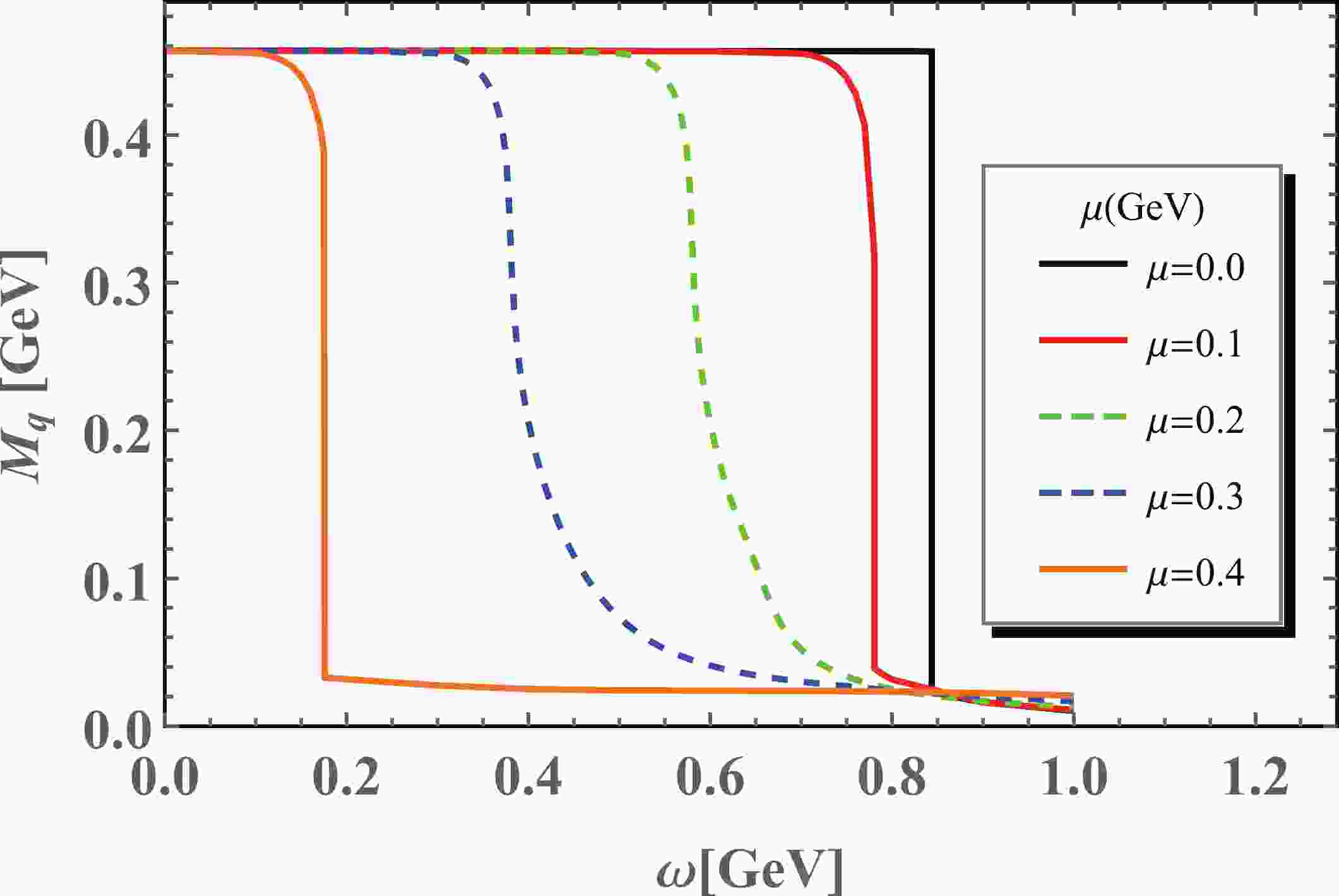
$r = 0.1\; {\rm GeV}^{-1}$ is calculated using$ M = m - 2G_S\left<\bar\psi\psi\right> $ , and the constituent quark mass as a function of angular velocity is shown in Fig. 1 for different chemical potentials. The chiral condensate exhibits a first order phase transition at large angular velocities for small chemical potentials, while this is exhibited at small angular velocities for large chemical potentials; this is in agreement with the results presented in [16], where a first order phase transition was observed in two corners of the three-dimensional$ T-\mu-\omega $ phase diagram.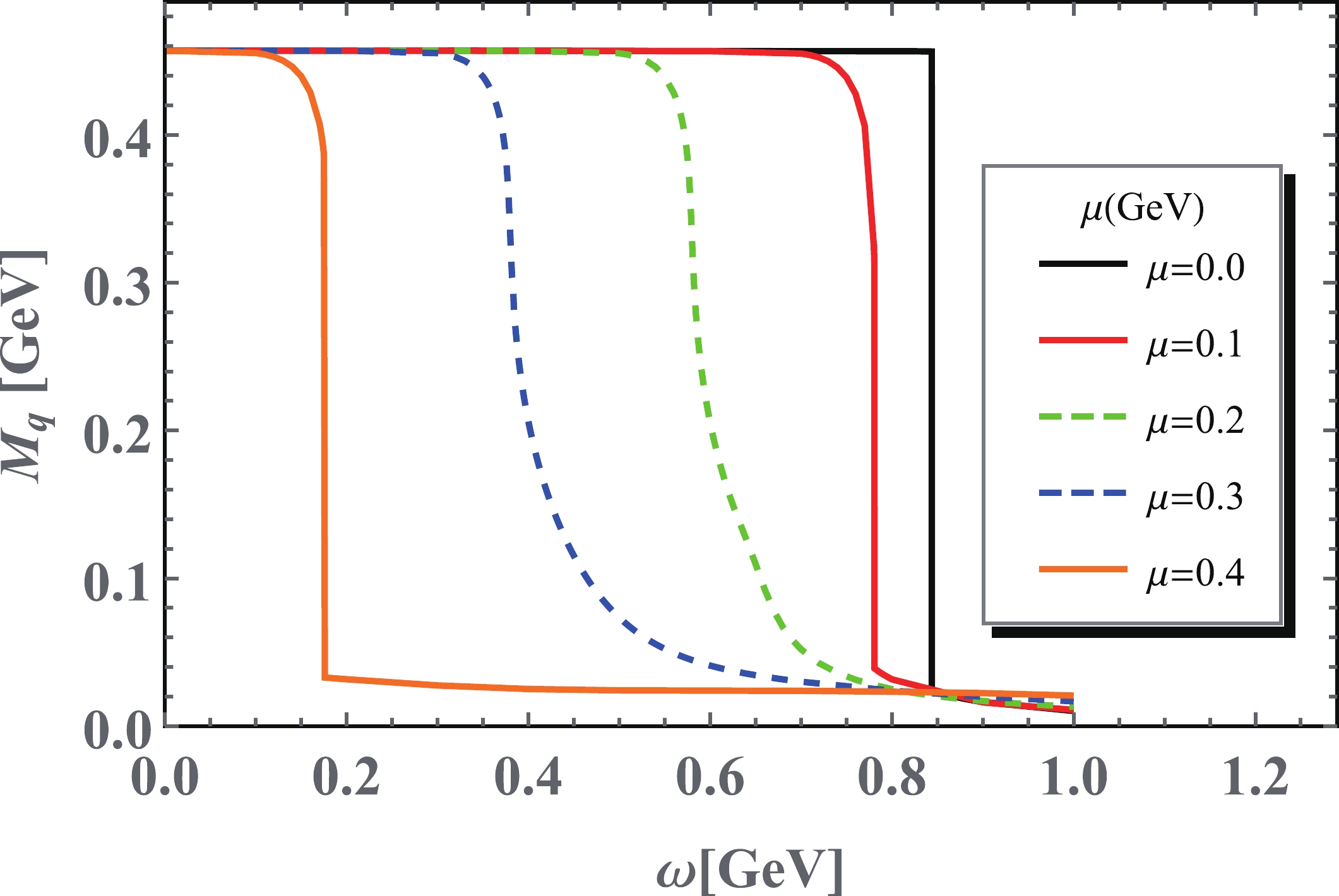
Figure 1. (color online) The constituent quark mass as a function of angular velocity for different chemical potentials.
From the numerical results, it is clear that the rotation speed and chemical potential are complementary when driven by chiral restoration. At low chemical potentials, the critical/crossover rotation speed is large. This decreases with increasing chemical potential. However it is clear that the chemical potential and rotation speed are not exactly equivalent because, physically, the chemical potential is the energy shift from the difference between the particle and anti-particle, while the shift induced by rotation polarization occurs from the difference between spin up and spin down. From this aspect, the
$ \pm \dfrac{1}{2}\omega $ could be treated as the spin chemical potential. Analytically, the difference may be explicitly observed in the gap equation and the polarization functions, as follows:$ \begin{aligned}[b] \\[-8pt] \Pi_{s}(0,{\rm i} \nu_{n}) = &N_{f}N_{c}\sum\limits_{s = \pm}\int\frac{{\rm d}^{3}\vec{p}}{(2\pi)^{3}}\left[ {\rm Res}1(\vec{p},\nu_{n}) \theta \left(-\mu -\frac{s\omega }{2}+E_{p}\right) n_{f}\left(E_{p}-\mu -\frac{s\omega }{2},T\right)\right.\\ &+{\rm Res}3(\vec{p},\nu_{n}) \theta \left(-\mu -\frac{s\omega }{2}+E_{p}\right) n_{f}\left(E_{p}-\mu -\frac{s\omega }{2},T\right)-{\rm Res}1(\vec{p},\nu_{n}) \theta \left(\mu +\frac{s\omega }{2}-E_{p}\right) n_{f}\left(-E_{p}+\mu +\frac{s\omega }{2},T\right)\\ & -{\rm Res}2(\vec{p},\nu_{n}) n_{f}\left(E_{p}+\mu +\frac{s\omega }{2},T\right)-{\rm Res}3(\vec{p},\nu_{n}) \theta \left(\mu +\frac{s\omega }{2}-E_{p}\right) n_{f}\left(-E_{p}+\mu +\frac{s\omega }{2},T\right)\\ & -{\rm Res}4(\vec{p},\nu_{n}) n_{f}\left(E_{p}+\mu +\frac{s\omega }{2},T\right)+{\rm Res}1(\vec{p},\nu_{n}) \theta \left(\mu +\frac{s\omega }{2}-E_{p}\right) +{\rm Res}3(\vec{p},\nu_{n}) \theta \left(\mu +\frac{s\omega }{2}-E_{p}\right)\\ &-{\rm Res}1\left(\vec{p},\nu_{n}\right)-{\rm Res}3\left(\vec{p},\nu_{n}\right) \Big], \end{aligned} $ 
(23) where
${\rm Res}1(\vec{p},\nu_{n}),{\rm Res}2(\vec{p},\nu_{n}),{\rm Res}3(\vec{p},\nu_{n})$ , and${\rm Res}4(\vec{p},\nu_{n})$ are residues in Eq. (40).The polarization function
$ \Pi_{ps} $ is given as$ \begin{aligned}[b] \Pi_{ps}(0,{\rm i} \nu_{n}) = &N_{f}N_{c}\sum\limits_{s = \pm}\int\frac{{\rm d}^{3}\vec{p}}{(2\pi)^{3}}\left[ {\rm Res}1'(\vec{p},\nu_{n}) \theta \left(-\mu -\frac{s\omega }{2}+E_{p}\right) n_{f}\left(E_{p}-\mu -\frac{s\omega }{2},T\right)\right.\\ &+{\rm Res}3'(\vec{p},\nu_{n}) \theta \left(-\mu -\frac{s\omega }{2}+E_{p}\right) n_{f}\left(E_{p}-\mu -\frac{s\omega }{2},T\right)-{\rm Res}1'(\vec{p},\nu_{n}) \theta \left(\mu +\frac{s\omega }{2}-E_{p}\right) n_{f}\left(-E_{p}+\mu +\frac{s\omega }{2},T\right) \\ &-{\rm Res}2'(\vec{p},\nu_{n}) n_{f}\left(E_{p}+\mu +\frac{s\omega }{2},T\right)-{\rm Res}3'(\vec{p},\nu_{n}) \theta \left(\mu +\frac{s\omega }{2}-E_{p}\right) n_{f}\left(-E_{p}+\mu +\frac{s\omega }{2},T\right) \end{aligned} $

$ \begin{aligned}[b] &-{\rm Res}4'(\vec{p},\nu_{n}) n_{f}\left(E_{p}+\mu +\frac{s\omega }{2},T\right)+{\rm Res}1'(\vec{p},\nu_{n}) \theta \left(\mu +\frac{s\omega }{2}-E_{p}\right) +{\rm Res}3'(\vec{p},\nu_{n}) \theta \left(\mu +\frac{s\omega }{2}-E_{p}\right)\\ &-{\rm Res}1'(\vec{p},\nu_{n})-{\rm Res}3'(\vec{p},\nu_{n})\Big]. \end{aligned} $

(24) Here,
${\rm Res}1'(\vec{p},\nu_{n}),\; {\rm Res}2'(\vec{p},\nu_{n}),\; {\rm Res}3'(\vec{p},\nu_{n})$ , and${\rm Res}4'(\vec{p}, $ $ \nu_{n})$ are residues in Eq. (A18).It is clear that the functions depend on both
$ \mu\pm\omega/2 $ combinations. However, it is also reasonable to assume that the critical behavior will occur at a rotation speed that satisfies$ E_p-\mu\pm\dfrac{\omega}{2} = 0 $ . If we choose a positive value for both the chemical potential and rotation speed, the$ \omega = 2(m-\mu) $ part would dominate the critical behavior. Hence, the chemical potential and rotation speed appear to be complementary when determining the critical point. -
Taking the direction of rotation as the z-axis, the three components of a massive vector meson can be represented as
$ s_{z} = \pm 1 $ and$ s_{z} = 0 $ . The nonzero spin components are polarized by the Barnett effect, which introduces the shift$ -{\vec\omega}\cdot{\vec S} $ to the energy levels under rotation. In our two-flavor model, we use the ρ meson to explore the rotation-induced energy shift with self-consistent numerical calculations at the quark level. Fig. 3 shows the numerical results for ρ masses with$ s_{z} = \pm 1 $ and$ s_{z} = 0 $ as functions of angular velocity at temperature$ T = 10 $ MeV. It is clear that the splitting mass curves reveal the different influences of rotation. In the$ s_z = 0 $ case, there is no net angular momentum for particle polarization by rotation. This indicates that the mass dependence on rotation is similar to the scalar case, which remains invariant while the chiral condensate is below the critical rotation speed. In the$ s_z = \pm 1 $ cases, the rotation polarization generates the energy shift$ \mp \omega $ for the corresponding masses; this is confirmed by the numerical results in Fig. 3. The mass dependence on the rotation speed is indicated by two straight lines for the$ s_z = \pm 1 $ components. The behavior could be analytically proven with an explicit form of the polarization functions. In the pole approximation, the masses are determined by the pole of the meson propagators, as in Eq. (19). With straightforward computation, as shown in the Appendix, the polarization functions of the vector meson satisfy
Figure 2. (color online) Scalar meson mass as a function of angular velocity at different chemical potentials and temperatures.
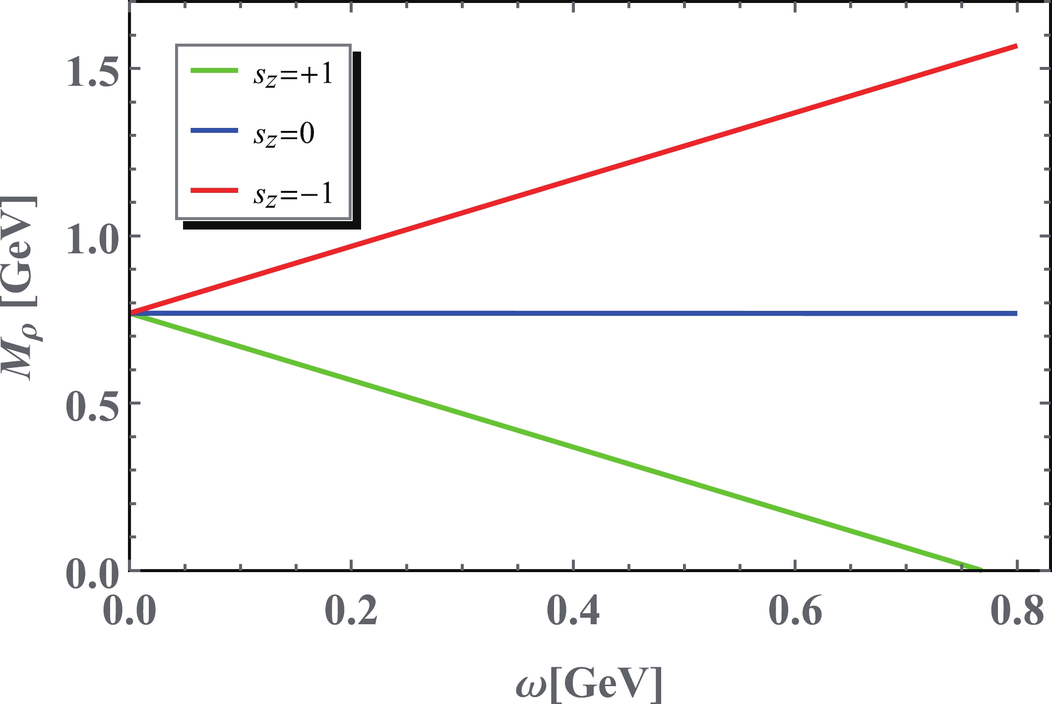
Figure 3. (color online) ρ meson masses as a function of angular velocity at temperature T=10 MeV.
$ \frac{1}{2}A_{1}^{2}(m_{\rho}+\omega)+\frac{1}{2}A_{2}^{2}(m_{\rho}-\omega) = A_{3}^{2}(m_{\rho}). $

(25) Therefore,
$ m_\rho(\omega = 0)-s_z\omega $ is the exact mass of the$ s_z = 0,\pm 1 $ components. The mass of the$ s_z = 1 $ spin component decreases linearly with angular velocity and reaches zero at the critical angular velocity$\omega_c = $ $ m_\rho(\omega = 0)$ . Beyond this, the$ s_z = 1 $ spin component of the vector meson will develop condensation in the vacuum, indicating that the system will be spontaneously spin polarized under strong rotation. -
Using the NJL model with vector channel interactions, we calculated scalar, pseudoscalar, and vector meson masses at a finite temperature, chemical potential, and rotation speed. In the RPA and pole approximation, the mesons are treated as the effective degree of freedoms, which transmit the interaction between quarks, and the masses are determined by the polarization functions. This approximation could explicitly preserve the Goldstone theorem; however, the meson back reaction to phase transitions is neglected. Because of the four-fermion point interaction and pole approximation, the microscopic details of mesons have been lost, and they all behave as fundamental particles that are polarized by rotation according to their net spin angular momentum. In the scalar and pseudoscalar cases, the mass spectra are controlled by the chiral condensate, which is the main mechanism generating hadron mass in the NJL model. At low temperatures and chemical potentials, chiral restoration is first order, which causes the meson masses to suddenly jump at the critical rotation speed. As the temperature or chemical potential increases, the phase transition degenerates to crossovers, which smoothens the meson mass curves along the rotation speed. At a large enough rotation speed, it is easy to expect that the vector condensate vacuum would be preferred and the corresponding effective mass would be zero. Therefore, we have only studied the behavior of vector meson masses below
$ \omega = m_\rho $ . Although the polarization function computation uses masses of the three components,$ s_z = 0, \pm 1 $ are the same as the results obtained by treating them as fundamental particles, that is,$ m_\rho $ and$ m_\rho\pm \omega $ . Once the chiral is restored, the vector condensate will emerge simultaneously, which will be investigated in our next study.In non-central heavy-ion collisions, the created system carries a large angular momentum, and the properties of particles will be changed in a rotating medium. In this paper, we investigated the behavior of scalar and vector meson mass under rotation. It is found that the behavior of scalar and pseudoscalar meson masses under angular velocity ω is similar to that at a finite chemical potential; both rely on the behavior of their constituent quark masses and reflect the property related to chiral symmetry. However, vector meson masses have a more profound relation to rotation. After tedious calculation, it turns out that, at low temperatures and a small chemical potential, the mass of the spin component
$ s_z = 0,\pm 1 $ of a vector meson under rotation exhibits a very simple mass splitting relation$ m_{\rho}^{s_z}(\omega) = m_\rho(\omega = 0)-\omega s_z $ similar to the Zeeman splitting of a charged meson in magnetic fields. In particular, the mass of the spin component$ s_z = 1 $ of the vector meson ρ decreases linearly with ω and reaches zero at$ \omega_c = m_\rho(\omega = 0) $ , which indicates that the system will develop$ s_z = 1 $ vector meson condensation and the system will be spontaneously spin-polarized under rotation. Further investigation is required to compare the spin polarization with$ s_z = 1 $ vector meson condensation and the spin polarization defined by the condensation of$< {\bar\psi}{\rm i}\sigma^{\mu\nu}\psi >$ proposed in [44-47].It should be noted that we did not consider inhomogeneous rotation and subtle boundary conditions in this study; for this first attempt, we chose a simplified scheme to introduce the qualitative
$ M(\omega) $ relation, which is easily estimated from the quark energy shift due to polarization effects induced by rotation. We can consider a more self-consistent treatment of$ M(\omega) $ in the near future. Even though the$ M(\omega) $ relation is simplified, we believe that this study is valuable, and, to the best of our knowledge, this is the first result for meson properties in a rotating background. This simplified result can be regarded as a reference, which can be compared with future results from lattice calculations and other effective models. -
We thank Kun Xu for useful discussions.
-
Rotating systems are not translationally invariant; however, a Green's function and polarization function can be defined in momentum space [22]. For the σ meson, the scalar polarization function under rotation is defined as [38,39]
$ \Pi_{s}(q) = -{\rm i} \int {\rm d}^{4}\tilde{r}{\rm Tr}_{sfc}\left[{\rm i} S(0;\tilde{r}){\rm i} S(\tilde{r};0)\right]{\rm e}^{{\rm i} q\cdot \tilde{r}} \tag{A1}$

where position
$ \tilde{r} $ can be expressed as$ (t,x,y,z) $ in Cartesian coordinates or$ (t,r,\phi,z) $ in cylindrical coordinates. Here, we have set$ \tilde{r}' = 0 $ for the propagators. Substituting Eq. (4) into the definition of the polarization function, a derivation can be expressed in cylindrical coordinates$ \begin{aligned}[b]\\[-8pt] \Pi_{s}(q) =& -{\rm i} N_{f} N_{c} \sum\limits_{n = -\infty}^{+\infty}\sum\limits_{l = -\infty}^{+\infty}\int {\rm d}^{4}\tilde{r} \int \frac{{\rm d} k_{0}{\rm d} k_{z}}{(2\pi)^{2}}\int_{0}^{+\infty}\frac{k_{t}{\rm d} k_{t}}{2\pi} \int \frac{{\rm d} p_{0}{\rm d} p_{z}}{(2\pi)^{2}} \int_{0}^{+\infty}\frac{p_{t}{\rm d} p_{t}}{2\pi} \\ &\times {\rm Tr}(A_{n}B_{l})\times \frac{{\rm e}^{-{\rm i}k_{0}t+ {\rm i}k_{z}z} {\rm e}^{{\rm i} n\phi}}{\left[k_{0}+\left(n+\dfrac{1}{2}\right)\omega\right]^{2}-k_{t}^{2}-k_{z}^{2}-M^{2}+{\rm i}\epsilon} \times \frac{{\rm e}^{{\rm i}p_{0}t-{\rm i}p_{z}z}{\rm e}^{-{\rm i} l\phi}}{\left[p_{0}+\left(l+\dfrac{1}{2}\right)\omega\right]^{2}-p_{t}^{2}-p_{z}^{2}-M^{2}+{\rm i}\epsilon}\times {\rm e}^{{\rm i} q\cdot \tilde{r}}, \end{aligned} \tag{A2}$ 
where
$ \begin{aligned}[b] A_{n}& = \begin{array}{l} \begin{pmatrix} \begin{smallmatrix} \left(k_{0}+M+\left(n+\frac{1}{2}\right) \omega \right) J_n(k_t r) J_n(0) & 0 & -k_z J_n(k_t r) J_n(0) & {\rm i} k_t J_n(k_t r) J_{n+1}(0) \\ 0 & \left(k_0+M+\left(n+\frac{1}{2}\right) \omega \right) {\rm e}^{{\rm i} \phi } J_{n+1}(k_{t} r) J_{n+1}(0) & -{\rm i} {\rm e}^{{\rm i} \phi } k_{t} J_{n+1}(k_{t} r) J_n(0) & k_{z} {\rm e}^{{\rm i} \phi } J_{n+1}(k_{t} r) J_{n+1}(0) \\ k_{z} J_n(k_{t} r) J_n(0) & -{\rm i} k_{t} J_n(k_{t} r) J_{n+1}(0) & -\left(k_{0}-M+\left(n+\frac{1}{2}\right) \omega \right) J_n(k_{t} r) J_n(0) & 0 \\ {\rm i} {\rm e}^{{\rm i} \phi } k_{t} J_{n+1}(k_{t} r) J_n(0) & -k_{z} {\rm e}^{{\rm i} \phi } J_{n+1}(k_{t} r) J_{n+1}(0) & 0 & -\left(k_{0}-M+\left(n+\frac{1}{2}\right) \omega \right) {\rm e}^{{\rm i} \phi } J_{n+1}(k_{t} r) J_{n+1}(0)\\ \end{smallmatrix} \end{pmatrix}, \end{array}\\ B_{l}& = \begin{array} {l} \begin{pmatrix} \begin{smallmatrix} \left(M+p_{0}+\left(l+\frac{1}{2}\right) \omega \right) J_l(p_{t} r) J_l(0) & 0 & -p_{z} J_l(p_{t} r) J_l(0) & {\rm i} p_{t} {\rm e}^{-{\rm i} \phi } J_{l+1}(p_{t} r) J_l(0) \\ 0 & \left(M+p_{0}+\left(l+\frac{1}{2}\right) \omega \right) {\rm e}^{-{\rm i} \phi } J_{l+1}(p_{t} r) J_{l+1}(0) & -{\rm i} p_{t} J_l(p_{t} r) J_{l+1}(0) & p_{z} {\rm e}^{-{\rm i} \phi } J_{l+1}(p_{t} r) J_{l+1}(0)\\ p_{z} J_l(p_{t} r) J_l(0) & -{\rm i} p_{t} {\rm e}^{-{\rm i} \phi } J_{l+1}(p_{t} r) J_l(0) & -\left(-M+p_{0}+\left(l+\frac{1}{2}\right) \omega \right) J_l(p_{t} r) J_l(0) & 0\\ {\rm i} p_{t} J_l(p_{t} r) J_{l+1}(0) & -p_{z} {\rm e}^{-{\rm i} \phi } J_{l+1}(p_{t} r) J_{l+1}(0) & 0 & -\left(-M+p_{0}+\left(l+\frac{1}{2}\right) \omega \right) {\rm e}^{-{\rm i} \phi } J_{l+1}(p_{t} r) J_{l+1}(0)\\ \end{smallmatrix} \end{pmatrix}. \end{array} \end{aligned} \tag{A3}$

Here, we provide a matrix form instead of the summation of the projection operators in Eq. (4). The term "
${\rm Tr}_{sfc}$ " represents the evaluation of the trace on the spinor, flavor, and color space. After simplification calculations, we get$ \begin{aligned}[b] {\rm Tr}(A_{n}B_{l}) =& \left[\frac{1}{2} (2 k_{0}+2 n \omega +\omega ) (2 l \omega +2 p_{0}+\omega )+2 M^2 -2 k_{z} p_{z}\right] J_l(0) J_n(0) J_n(k_{t} r) J_l(p_{t} r)\\ &+\left[\frac{1}{2} (2 k_{0}+2 n \omega +\omega ) (2 l \omega +2 p_{0}+\omega )+2 M^2 -2 k_{z} p_{z}\right]J_{l+1}(0) J_{n+1}(0) J_{n+1}(k_{t} r) J_{l+1}(p_{t} r)\\ &-2 k_{t} p_{t} J_{l+1}(0) J_{n+1}(0) J_n(k_{t} r) J_l(p_{t} r)-2 k_{t} p_{t} J_l(0) J_n(0) J_{n+1}(k_{t} r) J_{l+1}(p_{t} r). \end{aligned} \tag{A4}$

When
$ n\neq 0 $ , it is clear that$ J_{n}(0) = 0 $ and$ J_{0}(0) = 1 $ . As a consequence, the result of the summation will have finite terms.$ \begin{aligned}[b] \Pi_{s}(q) =& -{\rm i} \int {\rm d}^{4}\tilde{r} {\rm Tr}_{sfc}\left[S(0;\tilde{r})S(\tilde{r};0)\right]{\rm e}^{{\rm i} q\cdot \tilde{r}} = -{\rm i} N_{f}N_{c}\int {\rm d}^{4}\tilde{r} \int \frac{{\rm d} k_{0}{\rm d} k_{z}}{(2\pi)^{2}}\int_{0}^{+\infty}\frac{k_{t}{\rm d} k_{t}}{2\pi} \int \frac{{\rm d} p_{0}{\rm d} p_{z}}{(2\pi)^{2}} \int_{0}^{+\infty}\frac{p_{t}{\rm d} p_{t}}{2\pi} \\ &\times \left\{ \left[\frac{1}{2} (2 k_{0}+\omega ) ( 2 p_{0}+\omega )+2 M^{2}-2 k_{z} p_{z}\right] \times \frac{J_{0}(k_{t} r)J_{0}(p_{t}r){\rm e}^{-{\rm i} k_{0}t+{\rm i} k_{z}z}{\rm e}^{{\rm i} p_{0}t-{\rm i} p_{z}z}}{\left[\left(k_{0}+\dfrac{1}{2}\omega\right)^{2}-k_{t}^{2}-k_{z}^{2}-M^{2}+{\rm i}\epsilon\right] \left[\left(p_{0}+\dfrac{1}{2}\omega\right)^{2}-p_{t}^{2}-p_{z}^{2}-M^{2}+{\rm i}\epsilon\right]}\right.\\ &+\left[\frac{1}{2} (2 k_{0}-\omega ) ( 2 p_{0}-\omega )+2 M^{2}-2 k_{z} p_{z}\right]\times\frac{J_{0}(k_{t} r)J_{0}(p_{t}r){\rm e}^{-{\rm i} k_{0}t+{\rm i} k_{z}z}{\rm e}^{{\rm i} p_{0}t-{\rm i} p_{z}z}}{\left[\left(k_{0}-\dfrac{1}{2}\omega\right)^{2}-k_{t}^{2}-k_{z}^{2}-M^{2}+{\rm i}\epsilon\right] \left[\left(p_{0}-\dfrac{1}{2}\omega\right)^{2}-p_{t}^{2}-p_{z}^{2}-M^{2}+i\epsilon\right]}\\ &-2k_{t}p_{t}\times\frac{J_{1}(k_{t} r)J_{1}(p_{t}r){\rm e}^{-{\rm i} k_{0}t+{\rm i} k_{z}z}{\rm e}^{{\rm i} p_{0}t-{\rm i} p_{z}z}}{\left[\left(k_{0}+\dfrac{1}{2}\omega\right)^{2}-k_{t}^{2}-k_{z}^{2}-M^{2}+{\rm i}\epsilon\right] \left[\left(p_{0}+\dfrac{1}{2}\omega\right)^{2}-p_{t}^{2}-p_{z}^{2}-M^{2}+{\rm i}\epsilon\right]}\\ &-2k_{t}p_{t}\times\left.\frac{J_{-1}(k_{t} r)J_{-1}(p_{t}r){\rm e}^{-{\rm i} k_{0}t+{\rm i} k_{z}z}{\rm e}^{{\rm i} p_{0}t-{\rm i} p_{z}z}}{\left[\left(k_{0}-\dfrac{1}{2}\omega\right)^{2}-k_{t}^{2}-k_{z}^{2}-M^{2}+{\rm i}\epsilon\right] \left[\left(p_{0}-\dfrac{1}{2}\omega\right)^{2}-p_{t}^{2}-p_{z}^{2}-M^{2}+{\rm i}\epsilon\right]} \right\}\times {\rm e}^{{\rm i} q\cdot \tilde{r}}. \end{aligned}\tag{A5} $

Applying the integral representation of the Bessel functions, the polarization function can be simplified. In integral representation, Bessel functions are expressed as
$ \begin{aligned}[b] J_{n}(r)& = \frac{1}{2\pi}\int_{-\pi}^{+\pi}{\rm e}^{{\rm {\rm i}}(r\sin\theta-n\theta)}{\rm d}\theta,\\ J_{0}(r)& = \frac{1}{2\pi}\int_{0}^{2\pi}{\rm e}^{\pm {\rm i} r\cos\theta}{\rm d}\theta,\\ J_{1}(r)& = \frac{1}{2\pi {\rm i}}\int_{0}^{2\pi}{\rm e}^{{\rm i} r\cos\theta\pm {\rm i}\theta}{\rm d}\theta,\\ J_{1}(r)& = -\frac{1}{2\pi {\rm i}}\int_{0}^{2\pi}{\rm e}^{-{\rm i} r\cos\theta\pm {\rm i}\theta}{\rm d}\theta. \end{aligned}\tag{A6} $

Let
$ \vec{k_{t}} = (k_{t},\phi+\theta) = (k_{x},k_{y}),\vec{r} = (r,\phi) = (x,y) $ , and then we have the transformation formulae$ \int_{0}^{\infty}\frac{k_{t}{\rm d} k_{t}}{2\pi}\int_{0}^{2\pi}\frac{{\rm d}\theta}{2\pi {\rm i}}{\rm i} k_{t}{\rm e}^{{\rm i} \phi}{\rm e}^{{\rm i} k_{t}r \cos \theta+{\rm i} \theta} = \int \frac{{\rm d} k_{x}{\rm d} k_{y}}{(2\pi)^2}(k_{x}+{\rm i} k_{y}){\rm e}^{{\rm i}\vec{k_{t}}\cdot \vec{r}}, \tag{A7}$

$ \int_{0}^{\infty}\frac{k_{t}{\rm d} k_{t}}{2\pi}\int_{0}^{2\pi}\frac{{\rm d}\theta}{2\pi {\rm i}}{\rm i} k_{t}{\rm e}^{-{\rm i} \phi}{\rm e}^{-{\rm i} k_{t}r \cos \theta-{\rm i} \theta} = \int \frac{{\rm d} k_{x}{\rm d} k_{y}}{(2\pi)^2}(k_{x}-{\rm i} k_{y}){\rm e}^{-{\rm i}\vec{k_{t}}\cdot \vec{r}}. \tag{A8}$

After the transformation formulae are applied, the polarization function for scalar mesons can be expressed without the Bessel function. This will be more efficient for numerical calculations.
$ \begin{aligned}[b] \Pi_{s}(q) =& -{\rm i} N_{f}N_{c}\int {\rm d}^{4}\tilde{r} \int \frac{{\rm d}^{4} k}{(2\pi)^{4}} \int \frac{{\rm d}^{4} p}{(2\pi)^{4}} \\ &\times \left\{ \left[\frac{1}{2} (2 k_{0}+\omega ) ( 2 p_{0}+\omega )+2 M^{2}-2 k_{z} p_{z}\right] \times \frac{{\rm e}^{-{\rm i} k\cdot\tilde{r}}{\rm e}^{{\rm i} p\cdot\tilde{r}}}{\left[\left(k_{0}+\dfrac{1}{2}\omega\right)^{2}-\vec{k}^{2}-M^{2}+{\rm i}\epsilon\right] \left[\left(p_{0}+\dfrac{1}{2}\omega\right)^{2}-\vec{p}^{2}-M^{2}+{\rm i}\epsilon\right]}\right.\\ &+ \left[\frac{1}{2} (2 k_{0}-\omega )( 2 p_{0}-\omega )+2 M^{2}-2 k_{z} p_{z}\right]\times\frac{{\rm e}^{-{\rm i} k\cdot\tilde{r}}{\rm e}^{{\rm i} p\cdot\tilde{r}}}{\left[\left(k_{0}-\dfrac{1}{2}\omega\right)^{2}-\vec{k}^{2}-M^{2}+{\rm i}\epsilon\right] \left[\left(p_{0}-\dfrac{1}{2}\omega\right)^{2}-\vec{p}^{2}-M^{2}+{\rm i}\epsilon\right]}\\ &-2(k_{x}+{\rm i} k_{y})(p_{x}-{\rm i} p_{y})\times \frac{{\rm e}^{-{\rm i} k\cdot\tilde{r}}{\rm e}^{{\rm i} p\cdot\tilde{r}}}{\left[\left(k_{0}+\dfrac{1}{2}\omega\right)^{2}-\vec{k}^{2}-M^{2}+{\rm i}\epsilon\right] \left[\left(p_{0}+\dfrac{1}{2}\omega\right)^{2}-\vec{p}^{2}-M^{2}+{\rm i}\epsilon\right]}\\ &-2(k_{x}+{\rm i} k_{y})(p_{x}-{\rm i} p_{y})\times \frac{{\rm e}^{-{\rm i} k\cdot\tilde{r}}{\rm e}^{{\rm i} p\cdot\tilde{r}}}{\left[\left(k_{0}-\dfrac{1}{2}\omega\right)^{2}-\vec{k}^{2}-M^{2}+{\rm i}\epsilon\right] \left[\left(p_{0}-\dfrac{1}{2}\omega\right)^{2}-\vec{p}^{2}-M^{2}+{\rm i}\epsilon\right]} \}\times {\rm e}^{{\rm i} q\cdot \tilde{r}}.\\ \end{aligned} \tag{A9}$

Furthermore, by integrating
$ \tilde{r} $ and k analytically, we can obtain the polarization function, as follows:$ \begin{aligned}[b] \Pi_{s}(q) =& -{\rm i} N_{f}N_{c}\int \frac{{\rm d}^{4} p}{(2\pi)^{4}} \left\{ \frac{\left[2 \left(p_{0}+q_{0}+\dfrac{1}{2}\omega \right) \left( p_{0}+\dfrac{1}{2}\omega \right)+2 M^{2}-2 (p_{z}+q_{z}) p_{z}\right]-2\left[(p_{x}+q_{x})+{\rm i} (p_{y}+q_{y})\right](p_{x}-{\rm i} p_{y})} {\left[\left(p_{0}+q_{0}+\dfrac{1}{2}\omega\right)^{2}-(\vec{p}+\vec{q})^{2}-M^{2}+{\rm i}\epsilon\right] \left[\left(p_{0}+\dfrac{1}{2}\omega\right)^{2}-\vec{p}^{2}-M^{2}+{\rm i}\epsilon\right]}\right.\\ &+ \left.\frac{\left[2 \left(p_{0}+q_{0}-\dfrac{1}{2}\omega \right) \left( p_{0}-\dfrac{1}{2}\omega \right)+2 M^{2}-2 (p_{z}+q_{z}) p_{z}\right]-2\left[(p_{x}+q_{x})+{\rm i} (p_{y}+q_{y})\right](p_{x}-{\rm i} p_{y})} {\left[\left(p_{0}+q_{0}-\dfrac{1}{2}\omega\right)^{2}-(\vec{p}+\vec{q})^{2}-M^{2}+{\rm i}\epsilon\right] \left[\left(p_{0}-\dfrac{1}{2}\omega\right)^{2}-\vec{p}^{2}-M^{2}+{\rm i}\epsilon\right]} \right\}. \end{aligned}\tag{A10} $

Due to the symmetric integration analysis, the expression can be simplified, as follows:
$ \begin{aligned}[b] \Pi_{s}(q^2) =& -2 {\rm i} N_{f}N_{c}\int \frac{{\rm d}^{4} p}{(2\pi)^{4}} \left\{ \frac{\left (p_{0}+q_{0}+\dfrac{1}{2}\omega \right) \left(p_{0}+\dfrac{1}{2}\omega \right)+M^2-(\vec{p}+\vec{q}) \vec{p}} {\left[\left(p_{0}+q_{0}+\dfrac{1}{2}\omega\right)^{2}-(\vec{p}+\vec{q})^{2}-M^{2}\right] \left[\left(p_{0}+\dfrac{1}{2}\omega\right)^{2}-\vec{p}^{2}-M^{2}\right]}\right.\\ &+ \left.\frac{\left(p_{0}+q_{0}-\dfrac{1}{2}\omega \right) \left(p_{0}-\dfrac{1}{2}\omega \right)+M^2-(\vec{p}+\vec{q}) \vec{p}} {\left[\left(p_{0}+q_{0}-\dfrac{1}{2}\omega\right)^{2}-(\vec{p}+\vec{q})^{2}-M^{2}\right] \left[\left(p_{0}-\dfrac{1}{2}\omega\right)^{2}-\vec{p}^{2}-M^{2}\right]} \right\}. \end{aligned} \tag{A11}$

For the finite temperature formalism,
$ p_{0}\rightarrow {\rm i} \tilde{\omega}_{N}, \quad q_{0}\rightarrow {\rm i} \nu_{n}, \quad \int \frac{p_{0}}{2\pi}\rightarrow {\rm i} T\sum\limits_{N}, \quad \tilde{\omega}_{N} = (2N+1)\pi T. \tag{A12}$

The polarization function at a finite temperature and chemical potential under rotation can be rewritten as
$ \Pi_{s}(\vec{q},{\rm i}\nu_{n}) = 2N_{f} N_{c}T \sum\limits_{s = \pm}\sum\limits_N\int \frac{{\rm d}^{3}\vec{p}}{(2\pi)^{3}} \frac{\left[({\rm i} \tilde{\omega}_{N}+{\rm i} \nu_{n})+\dfrac{1}{2}s\omega+\mu\right]\left({\rm i} \tilde{\omega}_{N}+\dfrac{1}{2}s\omega+\mu\right)+M^{2}-(\vec{p}+\vec{q})\cdot\vec{p}}{\left[\left({\rm i} \tilde{\omega}_{N}+{\rm i} \nu_{n}+\dfrac{1}{2}s\omega+\mu\right)^{2}-(\vec{p}+\vec{q})^{2}-M^{2}\right]\left[\left({\rm i} \tilde{\omega}_{N}+\dfrac{1}{2}s\omega+\mu\right)^{2}-\vec{p}^{2}-M^{2}\right]}. \tag{A13} $

Setting
$ \vec{q} = 0 $ , the Matsubara summation will give us a result in terms of the residue theorem.$ \begin{aligned}[b] \Pi_{s}(0,{\rm i} \nu_{n}) = &N_{f}N_{c}\sum\limits_{s = \pm}\int\frac{{\rm d}^{3}\vec{p}}{(2\pi)^{3}}\left[ {\rm Res}1(\vec{p},\nu_{n}) \theta \left(-\mu -\frac{s\omega }{2}+E_{p}\right) n_{f}\left(E_{p}-\mu -\frac{s\omega }{2},T\right)\right.\\ &+{\rm Res}3(\vec{p},\nu_{n}) \theta \left(-\mu -\frac{s\omega }{2}+E_{p}\right) n_{f}\left(E_{p}-\mu -\frac{s\omega }{2},T\right)\\ &-{\rm Res}1(\vec{p},\nu_{n}) \theta \left(\mu +\frac{s\omega }{2}-E_{p}\right) n_{f}\left(-E_{p}+\mu +\frac{s\omega }{2},T\right) -{\rm Res}2(\vec{p},\nu_{n}) n_{f}\left(E_{p}+\mu +\frac{s\omega }{2},T\right)\\ &-{\rm Res}3(\vec{p},\nu_{n}) \theta \left(\mu +\frac{s\omega }{2}-E_{p}\right) n_{f}\left(-E_{p}+\mu +\frac{s\omega }{2},T\right) -{\rm Res}4(\vec{p},\nu_{n}) n_{f}\left(E_{p}+\mu +\frac{s\omega }{2},T\right)\\ &+{\rm Res}1(\vec{p},\nu_{n}) \theta \left(\mu +\frac{s\omega }{2}-E_{p}\right) +{\rm Res}3(\vec{p},\nu_{n}) \theta \left(\mu +\frac{s\omega }{2}-E_{p}\right)\\ &-{\rm Res}1\left(\vec{p},\nu_{n}\right)-{\rm Res}3\left(\vec{p},\nu_{n}\right) \Big], \end{aligned} \tag{A14}$

where
$n_{f}(x,T) = \dfrac{1}{{\rm e}^{x/T}+1}$ is the distribution function, and four residues are given, as follows:$ \begin{aligned}[b] {\rm Res}1(\vec{p},\nu_{n}) = &\frac{-{\rm i} \nu_{n} E_{p}+E_{p}^{2}+M^{2}-\vec{p}^{2}}{E_{p} \left(-\nu_{n}^2-2 {\rm i} \nu_{n} E_{p}\right)},\qquad {\rm Res}2(\vec{p},\nu_{n}) = \frac{-{\rm i} \nu_{n} E_{p}-E_{p}^{2}-M^{2}+\vec{p}^{2}}{E_{p} \left(-\nu_{n}^2+2 {\rm i} \nu_{n} E_{p}\right)},\\ {\rm Res}3(\vec{p},\nu_{n}) = &\frac{+{\rm i} \nu_{n} E_{p}+E_{p}^{2}+M^{2}-\vec{p}^{2}}{E_{p} \left(-\nu_{n}^2+2 {\rm i} \nu_{n} E_{p}\right)},\qquad {\rm Res}4(\vec{p},\nu_{n}) = \frac{{\rm i} \nu_{n} E_{p}-E_{p}^{2}-M^{2}+\vec{p}^{2}}{E_{p} \left(-\nu_{n}^2-2 {\rm i} \nu_{n} E_{p}\right)}. \end{aligned}\tag{A15} $

We should note that
$ E_{\mathit{\boldsymbol{p}}} = \sqrt{\mathit{\boldsymbol{p}}^{2}+M^{2}} $ , and the quark mass M is a function of angular velocity ω. For a psuadoscalar meson, the finite temperature version of the polarization function is$ \Pi_{ps}(\vec{q},{\rm i}\nu_{n}) = -4N_{f} N_{c}T \sum\limits_{s = \pm}\sum\limits_N\int \frac{{\rm d}^{3}\vec{p}}{(2\pi)^{3}} \frac{\left[({\rm i} \tilde{\omega}_{N}+{\rm i} \nu_{n})+\dfrac{1}{2}s\omega+\mu\right]\left[{\rm i} \tilde{\omega}_{N}+\dfrac{1}{2}s\omega+\mu\right]-M^{2}-(\vec{p}+\vec{q})\cdot\vec{p}}{\left[\left({\rm i} \tilde{\omega}_{N}+{\rm i} \nu_{n}+\dfrac{1}{2}s\omega+\mu\right)^{2}-(\vec{p}+\vec{q})^{2}-M^{2}\right]\left[\left({\rm i} \tilde{\omega}_{N}+\dfrac{1}{2}s\omega+\mu\right)^{2}-\vec{p}^{2}-M^{2}\right]}.\tag{A16} $

Seting
$ \vec{q} = 0 $ , the Matsubara summation gives$ \begin{aligned}[b] \Pi_{ps}(0,{\rm i} \nu_{n}) = &N_{f}N_{c}\sum\limits_{s = \pm}\int\frac{{\rm d}^{3}\vec{p}}{(2\pi)^{3}}\left[ {\rm Res}1'(\vec{p},\nu_{n}) \theta \left(-\mu -\frac{s\omega }{2}+E_{p}\right) n_{f}\left(E_{p}-\mu -\frac{s\omega }{2},T\right)\right.\\ &+{\rm Res}3'(\vec{p},\nu_{n}) \theta \left(-\mu -\frac{s\omega }{2}+E_{p}\right) n_{f}\left(E_{p}-\mu -\frac{s\omega }{2},T\right)\\ &-{\rm Res}1'(\vec{p},\nu_{n}) \theta \left(\mu +\frac{s\omega }{2}-E_{p}\right) n_{f}\left(-E_{p}+\mu +\frac{s\omega }{2},T\right) -{\rm Res}2'(\vec{p},\nu_{n}) n_{f}\left(E_{p}+\mu +\frac{s\omega }{2},T\right)\\ &-{\rm Res}3'(\vec{p},\nu_{n}) \theta \left(\mu +\frac{s\omega }{2}-E_{p}\right) n_{f}\left(-E_{p}+\mu +\frac{s\omega }{2},T\right) -{\rm Res}4'(\vec{p},\nu_{n}) n_{f}\left(E_{p}+\mu +\frac{s\omega }{2},T\right)\\ &+{\rm Res}1'(\vec{p},\nu_{n}) \theta \left(\mu +\frac{s\omega }{2}-E_{p}\right) +{\rm Res}3'(\vec{p},\nu_{n}) \theta \left(\mu +\frac{s\omega }{2}-E_{p}\right)\\ &-{\rm Res}1'(\vec{p},\nu_{n})-{\rm Res}3'(\vec{p},\nu_{n})\Big], \end{aligned}\tag{A17} $

where
$ \begin{aligned}[b] {\rm Res}1'(\vec{p},\nu_{n}) = &\frac{{\rm i} \nu_{n} E_{p}+E_{p}^{2}+M^{2}+\vec{p}^{2}}{E_{p} \left(-\nu_{n}^2-2 {\rm i} \nu_{n} E_{p}\right)},\qquad {\rm Res}2'(\vec{p},\nu_{n}) = \frac{{\rm i} \nu_{n} E_{p}+E_{p}^{2}-M^{2}-\vec{p}^{2}}{E_{p} \left(-\nu_{n}^2+2 {\rm i} \nu_{n} E_{p}\right)},\\ {\rm Res}3'(\vec{p},\nu_{n}) = &\frac{-{\rm i} \nu_{n} E_{p}-E_{p}^{2}+M^{2}+\vec{p}^{2}}{E_{p} \left(-\nu_{n}^2+2 {\rm i} \nu_{n} E_{p}\right)},\qquad {\rm Res}4'(\vec{p},\nu_{n}) = \frac{-{\rm i} \nu_{n} E_{p}+E_{p}^{2}-M^{2}-\vec{p}^{2}}{E_{p} \left(-\nu_{n}^2-2 {\rm i} \nu_{n} E_{p}\right)}. \end{aligned} \tag{A18}$

-
For a ρ meson, the polarization function with a one loop contribution can be expressed as
$ \Pi^{\mu\nu,ab} = -{\rm i} \int {\rm d}^{4}\tilde{r}{\rm Tr}_{sfc}\left[{\rm i} \gamma^{\mu}\tau^{a}S(0;\tilde{r}){\rm i} \gamma^{\nu}\tau^{b}S(\tilde{r};0)\right]{\rm e}^{{\rm i} q\cdot \tilde{r}}. \tag{B1}$

Using the approach introduced in Appendix A, it is clear that the charge of the ρ meson will make no difference with the polarization function under rotation. We can obtain the nonzero elements of the matrix
$ \Pi^{\mu\nu}_{\rho} = \left( \begin{array}{cccc} 0 & 0 & 0 & 0 \\ 0 & \Pi^{11} & \Pi^{12} & 0 \\ 0 & \Pi^{21} & \Pi^{22} & 0 \\ 0 & 0 & 0 & \Pi^{33} \\ \end{array} \right).\tag{B2} $

Using the same method in Appendix A and by setting
$ \vec{q} = 0 $ , we can obtain the nonzero elements$ \begin{aligned}[b] \Pi^{11}(q_{0})x =& N_{f}N_{c}\int \frac{{\rm d}^{4} p}{(2\pi)^{4}} \\ &\times \left\{-\frac{2 M^2-2 \left(p_{0}+\dfrac{\omega}{2}\right) \left(p_{0}+q_{0}-\dfrac{\omega}{2}\right)-2 p_{x}^2+2 p_{y}^2+2 p_{z}^2} {\left[\left(p_{0}+\dfrac{\omega }{2}\right)^2-\vec{p}^2-M^2\right] \left[\left(p_{0}+q_{0}-\dfrac{\omega }{2}\right)^2-\vec{p}^2-M^2\right]} -\frac{2 M^2-2 \left(p_{0}-\dfrac{\omega }{2}\right) \left(p_{0}+q_{0}+\dfrac{\omega }{2}\right)-2 p_{x}^2+2 p_{y}^2+2 p_{z}^2} {\left[\left(p_{0}-\dfrac{\omega }{2}\right)^2-\vec{p}^2-M^2\right] \left[\left(p_{0}+q_{0}+\dfrac{\omega }{2}\right)^2-\vec{p}^2-M^2\right]}\right\}, \end{aligned} \tag{B3}$ 
$ \begin{aligned}[b] \Pi^{12}(q_{0})=& -{\rm i} N_{f}N_{c}\int \frac{{\rm d}^{4} p}{(2\pi)^{4}} \\ &\times \left\{\frac{2 M^2-2 \left(p_{0}+\dfrac{\omega}{2}\right) \left(p_{0}+q_{0}-\dfrac{\omega}{2}\right)-2 p_{x}^2+2 p_{y}^2+2 p_{z}^2} {\left[\left(p_{0}+\dfrac{\omega }{2}\right)^2-\vec{p}^2-M^2\right] \left[\left(p_{0}+q_{0}-\dfrac{\omega }{2}\right)^2-\vec{p}^2-M^2\right]} -\frac{2 M^2-2 \left(p_{0}-\dfrac{\omega }{2}\right) \left(p_{0}+q_{0}+\dfrac{\omega }{2}\right)-2 p_{x}^2+2 p_{y}^2+2 p_{z}^2} {\left[\left(p_{0}-\dfrac{\omega }{2}\right)^2-\vec{p}^2-M^2\right] \left[\left(p_{0}+q_{0}+\dfrac{\omega }{2}\right)^2-\vec{p}^2-M^2\right]}\right\}, \end{aligned}\tag{B4} $

$ \begin{aligned}[b] \Pi^{21}(q_{0}) =& {\rm i} N_{f}N_{c}\int \frac{{\rm d}^{4} p}{(2\pi)^{4}} \\ &\times \left\{\frac{2 M^2-2 \left(p_{0}+\dfrac{\omega}{2}\right) \left(p_{0}+q_{0}-\dfrac{\omega}{2}\right)+2 p_{x}^2-2 p_{y}^2+2 p_{z}^2} {\left[\left(p_{0}+\dfrac{\omega }{2}\right)^2-\vec{p}^2-M^2\right] \left[\left(p_{0}+q_{0}-\dfrac{\omega }{2}\right)^2-\vec{p}^2-M^2\right]} -\frac{2 M^2-2 \left(p_{0}-\dfrac{\omega }{2}\right) \left(p_{0}+q_{0}+\dfrac{\omega }{2}\right)+2 p_{x}^2-2 p_{y}^2+2 p_{z}^2} {\left[\left(p_{0}-\dfrac{\omega }{2}\right)^2-\vec{p}^2-M^2\right] \left[\left(p_{0}+q_{0}+\dfrac{\omega }{2}\right)^2-\vec{p}^2-M^2\right]}\right\}, \end{aligned}\tag{B5} $

$ \begin{aligned}[b] \Pi^{22}(q_{0}) =& -N_{f}N_{c}\int \frac{{\rm d}^{4} p}{(2\pi)^{4}} \\ &\times \left\{\frac{2 M^2-2 \left(p_{0}+\dfrac{\omega}{2}\right) \left(p_{0}+q_{0}-\dfrac{\omega}{2}\right)-2 p_{x}^2+2 p_{y}^2+2 p_{z}^2} {\left[\left(p_{0}+\dfrac{\omega }{2}\right)^2-\vec{p}^2-M^2\right] \left[\left(p_{0}+q_{0}-\dfrac{\omega }{2}\right)^2-\vec{p}^2-M^2\right]} +\frac{2 M^2-2 \left(p_{0}-\dfrac{\omega }{2}\right) \left(p_{0}+q_{0}+\dfrac{\omega }{2}\right)-2 p_{x}^2+2 p_{y}^2+2 p_{z}^2} {\left[\left(p_{0}-\dfrac{\omega }{2}\right)^2-\vec{p}^2-M^2\right] \left[\left(p_{0}+q_{0}+\dfrac{\omega }{2}\right)^2-\vec{p}^2-M^2\right]}\right\}, \end{aligned} \tag{B6}$

$ \begin{aligned}[b] \Pi^{33}(q_{0}) =& -N_{f}N_{c}\int \frac{{\rm d}^{4} p}{(2\pi)^{4}} \\ &\times \left\{\frac{2 M^2-2 \left(p_{0}-\dfrac{\omega}{2}\right) \left(p_{0}+q_{0}-\dfrac{\omega}{2}\right)+2 p_{x}^2+2 p_{y}^2-2 p_{z}^2} {\left[\left(p_{0}-\dfrac{\omega }{2}\right)^2-\vec{p}^2-M^2\right] \left[\left(p_{0}+q_{0}-\dfrac{\omega }{2}\right)^2-\vec{p}^2-M^2\right]} +\frac{2 M^2-2 \left(p_{0}+\dfrac{\omega }{2}\right) \left(p_{0}+q_{0}+\dfrac{\omega }{2}\right)+2 p_{x}^2+2 p_{y}^2-2 p_{z}^2} {\left[\left(p_{0}+\dfrac{\omega }{2}\right)^2-\vec{p}^2-M^2\right] \left[\left(p_{0}+q_{0}+\dfrac{\omega }{2}\right)^2-\vec{p}^2-M^2\right]}\right\}. \end{aligned}\tag{B7} $

We rewrite the relation in Eq. (20).
$ \begin{aligned}[b] A_{1}^{2} = -(\Pi_{11} - {\rm i} \Pi_{12}),(s_{z} = -1 \text{ for } \rho \text{ meson }),\quad A_{2}^{2}= -\Pi_{11} - {\rm i} \Pi_{12},(s_{z} = +1\text{ for } \rho \text{ meson }),\quad A_{3}^{2} = -\Pi_{33},(s_{z} = 0 \text{ for } \rho \text{ meson }). \end{aligned} \tag{B8}$

The explicit form of the coefficients can be given by
$ A^{2}_{1}(q_{0}) = 2N_{f}N_{c}\int \frac{{\rm d}^{4} p}{(2\pi)^{4}} \frac{2 M^2-2 \left(p_{0}+\dfrac{\omega}{2}\right) \left(p_{0}+q_{0}-\dfrac{\omega}{2}\right)-2 p_{x}^2+2 p_{y}^2+2 p_{z}^2} {\left[\left(p_{0}+\dfrac{\omega }{2}\right)^2-\vec{p}^2-M^2\right] \left[\left(p_{0}+q_{0}-\dfrac{\omega }{2}\right)^2-\vec{p}^2-M^2\right]}, \tag{B9}$

$ A^{2}_{2}(q_{0}) = 2N_{f}N_{c}\int \frac{{\rm d}^{4} p}{(2\pi)^{4}} \frac{2 M^2-2 \left(p_{0}-\dfrac{\omega }{2}\right) \left(p_{0}+q_{0}+\dfrac{\omega }{2}\right)-2 p_{x}^2+2 p_{y}^2+2 p_{z}^2} {\left[\left(p_{0}-\dfrac{\omega }{2}\right)^2-\vec{p}^2-M^2\right] \left[\left(p_{0}+q_{0}+\dfrac{\omega }{2}\right)^2-\vec{p}^2-M^2\right]}, \tag{B10}$

$\begin{aligned}[b] A^{2}_{3}(q_{0}) =& N_{f}N_{c}\int \frac{{\rm d}^{4} p}{(2\pi)^{4}} \left\{\frac{2 M^2-2 \left(p_{0}-\dfrac{\omega}{2}\right) \left(p_{0}+q_{0}-\dfrac{\omega}{2}\right)+2 p_{x}^2+2 p_{y}^2-2 p_{z}^2} {\left[\left(p_{0}-\dfrac{\omega }{2}\right)^2-\vec{p}^2-M^2\right] \left[\left(p_{0}+q_{0}-\dfrac{\omega }{2}\right)^2-\vec{p}^2-M^2\right]}\right.\\ &+\left.\frac{2 M^2-2 \left(p_{0}+\dfrac{\omega }{2}\right) \left(p_{0}+q_{0}+\dfrac{\omega }{2}\right)+2 p_{x}^2+2 p_{y}^2-2 p_{z}^2} {\left[\left(p_{0}+\dfrac{\omega }{2}\right)^2-\vec{p}^2-M^2\right] \left[\left(p_{0}+q_{0}+\dfrac{\omega }{2}\right)^2-\vec{p}^2-M^2\right]}\right\}. \end{aligned}\tag{B11}$

Now, it is clear that
$ \frac{1}{2}A_{1}^{2}(m_{\rho}+\omega)+\frac{1}{2}A_{2}^{2}(m_{\rho}-\omega) = A_{3}^{2}(m_{\rho}). \tag{B12}$

Mass splitting of vector mesons and spontaneous spin polarization under rotation
- Received Date: 2021-09-01
- Available Online: 2022-02-15
Abstract: In this study, we investigate the effect of rotation on the masses of scalar and vector mesons in the framework of the 2-flavor Nambu-Jona-Lasinio model. The existence of rotation produces a tedious quark propagator and a corresponding polarization function. By applying the random phase approximation, the meson mass is numerically calculated. It is found that the behavior of scalar and pseudoscalar meson masses under angular velocity ω is similar to that at a finite chemical potential; both rely on the behavior of the constituent quark mass and reflect the property related to chiral symmetry. However, vector meson ρ masses have a more profound relation to rotation. After analytical and numerical calculations, it turns out that at low temperature and small chemical potential, the mass for spin component


 DownLoad: