


 Abstract
 HTML
HTML Reference
 Related
 PDF
PDF


-
Additional testing and development of the standard model (SM) and exploration of evidence for the existence of new physics (NP) beyond the SM are the most important research projects in the field of particle physics. The
$ B/D $ to light meson exclusive decay processes provide a good platform for these major research projects. The physical quantities of interest in these processes, such as the decay amplitude, decay width, and decay branching ratio, can usually be expressed in the form of a convolution of the distribution amplitudes (DAs) of the final state light mesons. Therefore, light meson DAs, particularly leading-twist DAs, are the key parameters for predicting these exclusive decay processes, and they also constitute the main error sources. Their accuracy is directly related to the theoretical prediction accuracy of such processes. The discussion on meson DAs began in 1980, when Lepage and Brodsky used collinear factorization to study the large momentum transition process [1]. In the following 40 years, the pionic leading-twist DA$ \phi_{2;\pi}(x,\mu) $ has attracted considerable attention. However, a completely consistent understanding of the pionic leading-twist DA behavior is still lacking.Generally, the pionic leading-twist DA
$ \phi_{2;\pi}(x,\mu) $ describes the momentum fraction distributions of partons in a pion in a particular Fock state, which is a universal nonperturbative object, and cannot be obtained directly through experiments. In principle, nonperturbative QCD methods should be used to study the pionic leading-twist DA. However, owing to the difficulty associated with nonperturbative QCD,$ \phi_{2;\pi}(x,\mu) $ is usually studied by combining nonperturbative QCD such as QCD sum rules and the lattice QCD theory (LQCD) with the phenomenological model [2, 3] or by combining the phenomenological model with relevant experimental data [4–7]. Evidently, the information regarding the pionic leading-twist DA obtained from the nonperturbative methods and related experiments must be expressed by the phenomenological model. The relevant literature highlights several phenomenological models commonly used to describe the pionic leading-twist DA behavior; these models include the truncation form of the Gegenbauer polynomial series based on$ \{C_n^{3/2}\} $ -basis (TF model), the light-cone harmonic oscillator model (LCHO model) [2–10] based on the Brodsky-Huang-Lepage (BHL) description [11], the form obtained from Dyson-Schwinger equations (DSE model) [12], the model derived from light-front holographic AdS/QCD (AdS/QCD model) [13, 14] , and the power-law parametrization form (PLP model) [15]. In addition, the pionic leading-twist DA has been studied using the light-front quark model [16, 17], the light-front constituent quark model [18], the nonlocal chiral-quark model (NLChQM) from the instanten vacuum [19], and the Nambu-Jona-Lasinio model [20–22] or by considering the infinite-momentum limit for the quasidistribution amplitude within NLChQM and LQCD based on the large-momentum effective theory [23].As a first-principles method, however, the computation of LQCD is usually limited to the first few moments of
$ \phi_{2;\pi}(x,\mu) $ [15, 24–33]. Owing to the systematic error arising from the truncation of the high-dimensional condensation terms and the approximation of the spectral density based on the quark-hadron duality, research on the pionic leading-twist DA using QCD sum rules is also limited to the lowest moments [34–44]. However, one can also abstract information on the pionic twist-2 DA via exclusive processes involving pions, such as the pion-photon transition form factor [45–52], pion electromagnetic form factor [53–56], and$ B/D\to \pi l\nu $ semileptonic decays [57–59]. The information regarding the pionic leading-twist DA obtained from nonperturbative methods and relevant experimental data is usually incomplete or indirect. Therefore, the choice of the phenomenological model is particularly important to accurately describe the behavior of the pionic leading-twist DA.Although the calculation of moments using nonperturbative methods is usually limited to the lowest orders, several studies that attempt to calculate adequate moments to obtain more complete information on the pionic leading-twist DA have been reported in the literature. For example, in the aforementioned DSE model, the first 50 x-moments are calculated by analyzing the corresponding gap and Bethe-Salpeter equations [12]. Very recently, to resolve the long-term limitation on the applications of the QCD sum rules, Li proposed a new dispersion relation for the moments of the pionic leading-twist DA [60] and obtained the first 18 Gegenbauer moments by solving the dispersion relation as an inverse problem in the inverse matrix method [61]. In Ref. [3], we studied the pionic leading-twist DA using QCD sum rules within the framework of the background field theory [62]. We clarified the fact that the sum rule of the zeroth ξ-moment of the pionic leading-twist DA cannot be normalized in the entire Borel parameter region, and we proposed a new sum rule formula for the nth ξ-moments. This new formula can reduce the systematic error of the sum rules of the ξ-moments, and it enables us to calculate higher-order moments. Following this, we calculated the values of the ξ-moments up to the 10th order and fitted those values with the LCHO model via the least squares method to determine the behavior of DA
$ \phi_{2;\pi}(x,\mu) $ . This method avoids the unreliability problem encountered in calculating the higher-order Gegenbauer moments of the DA by using the QCD sum rules. More ξ-moments create stronger constraints on the DA behavior. The research idea proposed in Ref. [3] improves the prediction ability of the QCD sum rules in the study of meson DAs and has been used to study the kaon leading-twist DA [63] and axial-vector$ a_1(1260) $ -meson longitudinal leading-twist DA [64]. Inspired by the results reported in Ref. [3], we attempt to calculate the values of more ξ-moments with orders higher than 10 and analyze several commonly used and relatively simple models from the literature, such as the TF model, LCHO model, DSE model, AdS/QCD model, and PLP model, using the least squares method.The remainder of this paper is organized as follows. In Sec. II, we provide a brief overview of several pionic leading-twist DA models to be analyzed. In Sec. III, we present the sum rules of the nth ξ-moment obtained in Ref. [3] for subsequent discussions. A numerical analysis is described in Sec. IV, and Sec. V provides a summary.
-
TF model By solving the renormalization group equation, the pionic leading-twist DA at a scale μ can be expanded into a Gegenbauer polynomial series [65, 66]. Its truncation form truncated from the Nth term may be the most common phenomenological model, and it is described as
$ \phi_{2;{\pi}}^{\rm TF}(x,\mu) = 6x(1-x) \left[ 1 + \sum^N_{n=2} a_n^{2;{\pi}}(\mu) C^{3/2}_n(2x-1) \right], $

(1) where
$ C^{3/2}_n(2x-1) $ is the nth order Gegenbauer polynomial, and the coefficient$ a_n^{2;{\pi}}(\mu) $ is the corresponding Gegenbauer moment. Owing to isospin symmetry, the odd Gegenbauer moments vanish, and only the even Gegenbauer moments are retained. The Gegenbauer moments$ a_n^{2;{\pi}}(\mu) $ can be calculated directly using nonperturbative LQCD [15, 24–33] or QCD sum rules [34–44]. However, owing to the limitations of LQCD and QCD sum rules and the fact that the stability of the Gegenbauer moments calculated based on these two nonperturbative methods decreases sharply with increasing order n [3], the ability of the TF model in describing the dependence on the parton momentum fraction x is difficult to improve. Therefore, the following two forms for the TF model have been usually adopted in the literature①:$ \phi_{2;{\pi}}^{\rm TF,I}(x,\mu) = 6x(1-x) \left[ 1 + a_2^{2;{\pi}}(\mu) C^{3/2}_2(2x-1) \right], $

(2) and
$ \begin{aligned}[b] \phi_{2;{\pi}}^{\rm TF,II}(x,\mu) =& 6x(1-x) \left[ 1 + a_2^{2;{\pi}}(\mu) C^{3/2}_2(2x-1) \right. \\ &+ \left. a_4^{2;{\pi}}(\mu) C^{3/2}_4(2x-1) \right]. \end{aligned} $

(3) LCHO model By using the approximate bound-state solution of a hadron in terms of the quark model as the starting point, BHL suggest that the hadronic wave function (WF) can be obtained by connecting the equal-time WF in the rest frame with the WF in the infinite-momentum frame. This is the so-called BHL description [11]. Based on the BHL description, the LCHO model for the pionic leading-twist DA is established and improved [2–10], and this can be expressed as [3]
$ \begin{aligned}[b] \phi_{2;\pi}^{\rm LCHO}(x,\mu_0) =& \frac{\sqrt{3} A_{2;\pi} \hat{m}_q \beta_{2;\pi}}{2\pi^{3/2}f_\pi} \sqrt{x(1-x)} \varphi_{2;\pi}(x) \\ &\times \left\{ \rm{Erf}\left[ \sqrt{\frac{\hat{m}_q^2 + \mu_0^2}{8\beta_{2;\pi}^2 x(1-x)}} \right] \right. \\ &- \left. \rm{Erf}\left[ \sqrt{\frac{\hat{m}_q^2}{8\beta_{2;\pi}^2 x(1-x)}} \right] \right\}, \end{aligned} $

(4) with the longitudinal distribution function
$ \varphi_{2;\pi}(x) = \left[ x(1-x) \right]^{\alpha_{2;\pi}} \left[ 1 + B_2^{2;\pi} C_2^{3/2}(2x-1) \right], $

(5) where
$ \hat{m}_q $ is the constituent u or d quark mass, and$ f_\pi $ is the pion decay constant. Several mass schemes for$ \hat{m}_q $ have been proposed in the literature. In Ref. [3], however, we find that by fitting the values of the ξ-moments with the LCHO model (4), the goodness of fit increases as$ \hat{m}_q $ decreases. Thus, we consider$ \hat{m}_q = 150\ {\rm MeV} $ in this paper. In addition,$ A_{2;\pi} $ is the normalization constant,$ \beta_{2;\pi} $ is a harmonious parameter, and${\rm Erf}(x) = 2\int^x_0 {\rm e}^{-t^2} {\rm d} x/{\sqrt{\pi}}$ is the error function. The LCHO model is based on four model parameters:$ A_{2;\pi} $ ,$ \beta_{2;\pi} $ ,$ \alpha_{2;\pi} $ , and$ B_2^{2;\pi} $ . Usually, two constraints are imposed: the DA normalization condition resulting from the process$ \pi \to \mu\nu $ , and the sum rule derived from the$ \pi^0 \to \gamma\gamma $ decay amplitude [3]. Only two model parameters are independent, which can be constrained by the ξ-moments [3] or experimental data [4–7].DSE model In Ref. [12], the authors suggest a new form of the pionic leading-twist DA by combining the truncation of the series of the Gegenbauer polynomials with order α,
$ C_n^\alpha(2x-1) $ , and$ [x(1-x)]^{\alpha_-} $ with$ \alpha_- = \alpha - 1/2 $ . Compared with the TF model based on the$ \{C_n^{3/2}\} $ -basis, its advantage is that one can accelerate the convergence of the procedure by optimizing α, reducing the non-zero coefficients, and reducing the introduced spurious oscillations. The parameters of the DSE model are determined by using the first$ 50 $ x-moments,$\left < x^n\right > = \int^1_0 {\rm d} x x^n \phi_{2;\pi}(x,\mu)$ , obtained by analyzing the corresponding gap and Bethe-Salpeter equations [12]. However, the results depend on the kernels. Evident differences are noted between the behaviors with the rainbow-ladder and dynamical-chiral-symmetry-breaking-improved kernels [12]. Based on Ref. [12], the DSE model for the pionic leading-twist DA is described as$ \phi^{\rm DSE}_{2;\pi}(x) = \mathcal{N} [x(1-x)]^{\alpha^{\rm DSE}_-} \left[ 1 + a_2^{\rm DSE} C_2^{\alpha^{\rm DSE}}(2x-1) \right], $

(6) where
$ \alpha^{\rm DSE}_- = \alpha^{\rm DSE} - 1/2 $ , and$ \mathcal{N} $ is the normalization constant. With the normalization condition of the pionic leading-twist DA,$ \mathcal{N} = 4^{\alpha^{\rm DSE}} \Gamma(\alpha^{\rm DSE} + 1) / \left[ \sqrt{\pi} \Gamma(\alpha^{\rm DSE} + 1/2) \right] $ .AdS/QCD model The light-front (LF) holographic AdS/QCD was developed more than 10 years ago [67–71], and it is a semiclassical first approximation to strongly coupled QCD. In this approach, a holographic duality exists between the hadron dynamics in physical four-dimensional spacetime at a fixed LF time
$ \tau = x^+ = x^0 + x^3 $ and the dynamics of the gravitational theory in five-dimensional anti-de Sitter (AdS) space. Based on the LF holographic AdS/QCD, Ref. [13] suggests two forms for the pionic leading-twist DA, which are described as$ \begin{aligned}[b] \phi^{\rm AdS,I}_{2;\pi}(x,\mu)=& \frac{\sqrt{3}}{\pi f_\pi} \int^{| {k}_\perp| < \mu} \frac{{\rm d}^2 {k}_\perp}{(2\pi)^2} \frac{N_1}{(x\bar{x})^{1/2}} \\ &\times \hat{m}_q \psi^{\rm AdS}_{2;\pi}(x, {k}_\perp), \end{aligned} $

(7) $ \begin{aligned}[b] \phi^{\rm AdS,II}_{2;\pi}(x,\mu) =& \frac{\sqrt{3}}{\pi f_\pi} \int^{| {k}_\perp| < \mu} \frac{{\rm d}^2 {k}_\perp}{(2\pi)^2} \frac{N_2}{(x\bar{x})^{1/2}} \\ &\times \left( \hat{m}_q + x\bar{x} \widetilde{m}_\pi \right) \psi^{\rm AdS}_{2;\pi}(x, {k}_\perp), \end{aligned} $

(8) with the radial WF
$ \psi^{\rm AdS}_{2;\pi}(x, {k}_\perp) = \frac{4\pi}{\sqrt{\lambda}} \frac{1}{\sqrt{x\bar{x}}} {\rm e}^{-\frac{ {k}^2_\perp}{2\lambda x\bar{x}}} {\rm e}^{-\frac{\hat{m}_q^2}{2\lambda x\bar{x}} }. $

(9) Here,
$ \sqrt{\lambda} $ is the mass scale parameter;$ {k}_\perp $ is the transverse momentum;$ N_1 $ and$ N_2 $ are the normalization constants and can be obtained with the normalization condition for$ \phi^{\rm AdS,I}_{2;\pi}(x,\mu) $ and$ \phi^{\rm AdS,II}_{2;\pi}(x,\mu) $ , respectively; and$ \widetilde{m}_\pi = \dfrac{\hat{m}_q^2 + {k}_\perp^2}{x(1-x)} $ is the invariant mass of the$ q\bar{q} $ pair in the pseudoscalar meson [14]. The difference between$ \phi^{\rm AdS,I}_{2;\pi}(x,\mu) $ and$ \phi^{\rm AdS,II}_{2;\pi}(x,\mu) $ can be attributed to the fact that the latter is constructed by further considering the impact of the Dirac structure such as$\not p \gamma_5$ on the spin WF. By substituting Eq. (9) into Eqs. (7) and (8) and after integrating over the transverse momentum$ {k}_\perp $ , the explicit forms of$ \phi^{\rm AdS,I}_{2;\pi}(x,\mu) $ and$ \phi^{\rm AdS,II}_{2;\pi}(x,\mu) $ can be obtained as$ \begin{aligned}[b] \phi^{\rm AdS,I}_{2;\pi}(x,\mu) =& \frac{2\sqrt{3}N_1\sqrt{\lambda}}{\pi f_\pi} \hat{m}_q \exp \left( -\frac{\hat{m}_q^2}{2\lambda x\bar{x}} \right) \\ &\times\left[ 1 - \exp \left( -\frac{\mu^2}{2\lambda x\bar{x}} \right) \right], \end{aligned} $

(10) $ \begin{aligned}[b] \phi^{\rm AdS,II}_{2;\pi}(x,\mu) =& \frac{2\sqrt{3}N_2\sqrt{\lambda}}{\pi f_\pi} \left( x\bar{x} \right)^{1/2} \left\{ \exp \left( - \frac{\hat{m}_q^2 + \mu^2}{2\lambda x\bar{x}} \right) \right. \\ &\times \left[ \hat{m}_q \exp \left( \frac{\mu^2}{2\lambda x\bar{x}} \right) \left( 1 + (x\bar{x})^{-1/2} \right) \right. \\ &-\left. \hat{m}_q (x\bar{x})^{-1/2} - \sqrt{\hat{m}_q^2 + \mu^2} \right] \\ &+ \sqrt{\frac{\pi}{2}} \sqrt{\lambda} \left( x\bar{x} \right)^{1/2} \left[ {\rm Erf} \left( \sqrt{\frac{\hat{m}_q^2 + \mu^2}{2\lambda x\bar{x}}} \right) \right. \\ &- \left.\left. {\rm Erf} \left( \sqrt{\frac{\hat{m}_q^2}{2\lambda x\bar{x}}} \right) \right] \right\}. \end{aligned} $

(11) As pointed out in Refs. [13, 72], the light-quark mass
$ \hat{m}_q $ in the AdS/QCD model is the effective quark mass obtained from the reduction of higher Fock states as functionals of the valence states. Hence, we do not fix it as in the LCHO model. Here,$ \hat{m}_q $ and$ \sqrt{\lambda} $ should be the undetermined parameters of the AdS/QCD model, and these can be extracted from observable measurements [13, 72, 73].PLP model By analyzing 35 different Coordinated Lattice Simulation ensembles with
$ N_f = 2+1 $ flavors of dynamical Wilson-Clover fermions, Ref. [15] presents the lattice determination for the first Gegenbauer moments of the pionic leading-twist DA and suggests a model for the pion leading-twist DA based on a simple power-law parametrization:$ \phi_{2;\pi}^{\rm PLP}(x) = \frac{\Gamma[2\alpha + 2]}{\Gamma[\alpha + 1]^2} x^\alpha (1-x)^\alpha. $

(12) Evidently, the PLP model
$ \phi_{2;\pi}^{\rm PLP}(x) $ satisfies the normalization condition owing to the coefficient$\Gamma[2\alpha + 2]/ \Gamma[\alpha + 1]^2$ . Recently, the PLP model was also used in Ref. [60] to fit the first 18 Gegenbauer moments by solving the dispersion relation as an inverse problem in the inverse matrix method [61] within the framework of the QCD sum rule method. -
Considering the fact that the sum rule of the zeroth order ξ-moment of the pionic leading-twist DA cannot be normalized in the entire Borel parameter region, we suggested the following form for the nth order ξ-moment in Ref. [3]:
$ \langle\xi^n\rangle_{2;\pi} = \frac{\langle\xi^n\rangle_{2;\pi} \langle \xi^0\rangle_{2;\pi}}{\sqrt{\langle \xi^0\rangle_{2;\pi}^2}}. $

(13) Here, the numerator is obtained based on the following sum rules:
$ \begin{aligned}[b]\\[-5pt] \frac{\langle\xi^n\rangle_{2;\pi} \langle \xi^0\rangle_{2;\pi} f_{\pi}^2}{M^2 {\rm e}^{m_\pi^2/M^2}} =& \frac{3}{4\pi^2} \frac{1}{(n+1)(n+3)} \Big( 1 - {\rm e}^{-s_\pi/M^2} \Big) + \frac{(m_d + m_u) \langle\bar{q}q \rangle }{(M^2)^2} \; +\; \frac{\langle \alpha_sG^2\rangle }{(M^2)^2}\; \frac{1 + n\theta(n-2)}{12\pi(n+1)} \\ & - \frac{(m_d + m_u)\langle g_s\bar{q}\sigma TGq \rangle }{(M^2)^3}\frac{8n+1}{18} + \frac{\langle g_s\bar{q}q\rangle ^2}{(M^2)^3} \frac{4(2n+1)}{81} - \frac{\langle g_s^3fG^3\rangle }{(M^2)^3}\frac{n \theta(n-2)}{48\pi^2} + \frac{\langle g_s^2\bar{q}q\rangle ^2}{(M^2)^3} \frac{2+\kappa^2}{486\pi^2} \\ & \times \Big\{ -2(51n+ 25)\Big( -\ln \frac{M^2}{\mu^2} \Big) + 3(17n+35) + \theta(n-2)\Big[ 2n \Big( -\ln \frac{M^2}{\mu^2} \Big) + \frac{49n^2 +100n+56}n \\ & - 25(2n+1)\Big[ \psi\Big(\frac{n+1}{2}\Big) - \psi\Big(\frac{n}{2}\Big) + \ln4 \Big] \Big] \Big\}. \end{aligned} $ 
(14) The denominator in Eq. (13) can be obtained by substituting
$ n = 0 $ in Eq. (14), i.e.,$ \begin{aligned}[b] \frac{\langle \xi^0\rangle_{2;\pi} ^2 f_{\pi}^2}{M^2 {\rm e}^{m_\pi^2/M^2}} =& \frac{1}{4\pi^2} \Big( 1 - {\rm e}^{-s_\pi / M^2} \Big) + (m_d + m_u)\; \frac{ \langle \bar{q}q \rangle }{(M^2)^2} \\ & + \frac{\langle \alpha_sG^2\rangle }{(M^2)^2} \frac{1}{12\pi} - \frac{1}{18}(m_d + m_u) \frac{ \langle g_s\bar{q}\sigma TGq \rangle }{(M^2)^3} \\ &+ \frac{4}{81} \frac{\langle g_s\bar{q}q\rangle ^2}{(M^2)^3} + \frac{\langle g_s^2\bar{q}q\rangle ^2}{(M^2)^3} \frac{2+\kappa^2}{486\pi^2}\\ &\times \Big[ -50 \Big( -\ln \frac{M^2}{\mu^2} \Big) + 105 \Big]. \end{aligned} $

(15) In Eqs. (14) and (15),
$ m_\pi $ is the mass of a pion, M is the Borel parameter,$ m_{u(d)} $ is the current$ u(d) $ quark mass,$s_\pi \simeq 1.05~{\rm GeV}^2$ [3] is the continuum threshold, and$ \psi(x) $ is the digamma function. In addition,$ \langle \bar{q}q \rangle $ ,$ \langle \alpha_sG^2 \rangle $ ,$ \langle g_s\bar{q}\sigma TGq \rangle $ , and$ \langle g_s^3fG^3\rangle $ are the double-quark condensate, double-gluon condensate, quark-gluon mixed condensate, and triple-gluon condensate, respectively;$ \langle g_s\bar{q}q\rangle ^2 $ and$ \langle g_s^2\bar{q}q\rangle ^2 $ are two four-quark condensates; and κ is the ratio of the double s quark condensate and double$ u/d $ quark condensate.As discussed in Ref. [3], the sum rules in Eq. (13) can provide more accurate values for the ξ-moments, owing to the elimination of some systematic errors caused by the continuum state, the absence of high-dimensional condensates, and various input parameters. In particular, we obtain appropriate Borel windows for the first five nonzero ξ-moments of the pionic leading-twist DA by constraining the dimension-six contribution for all
$ \left<\xi^n\right>_{2;\pi} $ to be no more than$5$ % and the continuum contribution of$ \left<\xi^n\right>_{2;\pi} $ to be less than$(30,35,40,40,40)$ % for$ n = (2,4,6,8,10) $ [3]. This, in turn, implies that the systematic error caused by the missing higher-dimension condensates and the continuum and excited states under the quark-hadron duality approximation does not increase with the increasing order n. Following this, the sum rules (13) indeed alleviate the limitation of the system error on the prediction ability of the QCD sum rule method for higher-order ξ-moments. Inspired by this, we calculate the ξ-moments$ \left<\xi^n\right>_{2;\pi} (n = 12, 14, 16, 18, 20) $ in the next section. Based on the criteria set to obtain the allowable Borel windows for these ξ-moments, one can find that the values of the ξ-moments$ \left<\xi^n\right>_{2;\pi} (n = 12, 14, 16, 18, 20) $ obtained in the next section are credible. -
The first five nonzero ξ-moments of the pionic leading-twist DA have been calculated using the sum rules in Eq. (13) in Ref. [3], and these can be summarized as
$ \begin{aligned}[b] \left<\xi^2\right>_{2;\pi} =& 0.271 \pm 0.013, \quad \left<\xi^4\right>_{2;\pi} =0.138 \pm 0.010, \\ \left<\xi^6\right>_{2;\pi} =& 0.087 \pm 0.006, \quad \left<\xi^8\right>_{2;\pi} = 0.064 \pm 0.007, \\ \left<\xi^{10}\right>_{2;\pi} =& 0.050 \pm 0.006 \end{aligned} $

(16) on the scale of
$\mu = 1~{\rm GeV}$ .To calculate the values of the ξ-moments
$ \left<\xi^n\right>_{2;\pi} (n = 12, 14, 16, 18, 20) $ , we consider the same inputs as those in Ref. [3], i.e.,$ \begin{aligned}[b] m_\pi =& 139.57039 \pm 0.00017 {\rm MeV}, \\ f_\pi =& 130.2 \pm 1.2 ~{\rm MeV}, \\ m_u =& 2.16^{+0.49}_{-0.26}~ {\rm MeV}, \\ m_d =& 4.67^{+0.48}_{-0.17} ~{\rm MeV}, \\ \left<\bar{q}q\right> =& \left( -289.14^{+9.34}_{-4.47} \right)^3 ~{\rm MeV}^3, \\ \left<g_S \bar{q}\sigma TGq \right> =& \left( -1.934^{+0.188}_{-0.103} \right) \times 10^{-2} ~{\rm GeV}^5, \\ \left<g_s\bar{q}q\right>^2 =& \left( 2.082^{+0.734}_{-0.697} \right) \times 10^{-3} ~{\rm GeV}^6, \\ \left<g_s^2\bar{q}q\right>^2 =& \left( 7.420^{+2.614}_{-2.483} \right) \times 10^{-3} ~{\rm GeV}^6, \\ \left<\alpha_sG^2\right> =& 0.038 \pm 0.011 ~{\rm GeV}^4, \\ \left<g_s^3 fG^3 \right>\simeq& 0.045 ~{\rm GeV}^6, \\ \kappa =& 0.74\pm 0.03, \end{aligned} $

(17) on the scale of
$\mu = 2~{\rm GeV}$ . For the scale evolutions of the above inputs, readers can refer to Ref. [3].Substituting the inputs presented in Eq. (17) into the sum rules in Eq. (13), the ξ-moments
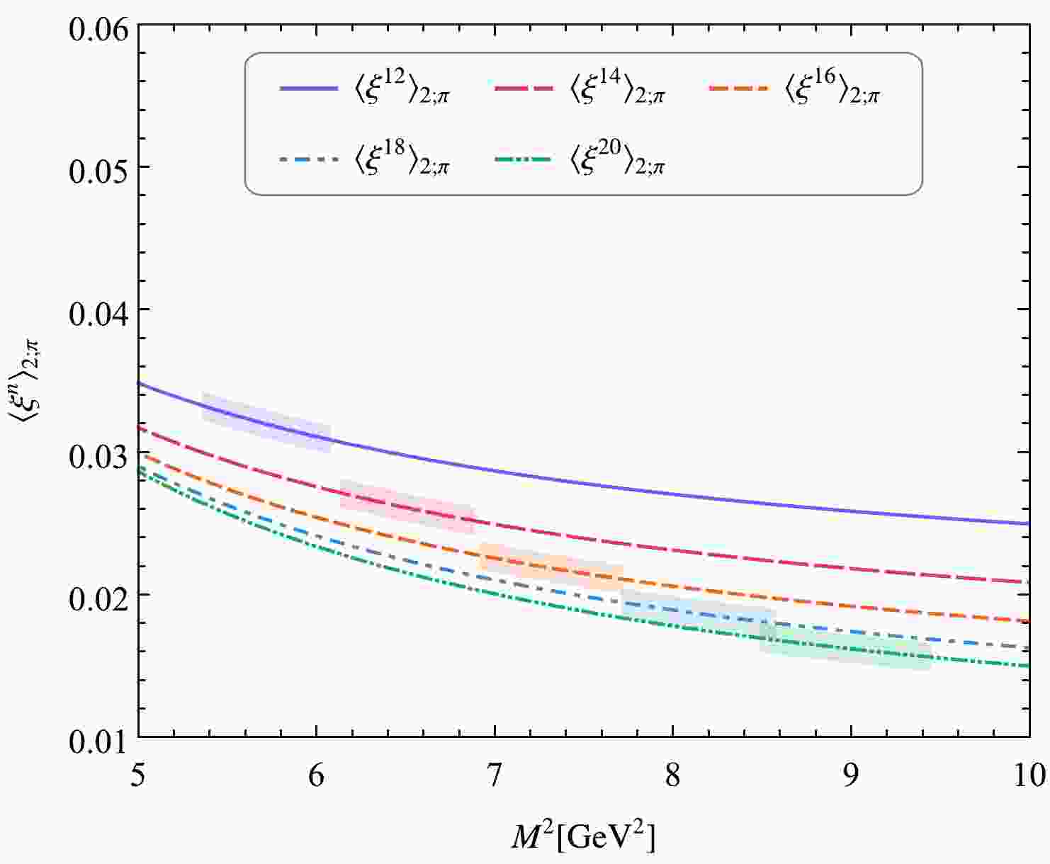
$ \left<\xi^n\right>_{2;\pi} (n = $ 12, 14, 16, 18, 20) and the corresponding contributions from the continuum states and dimension-six condensates versus the Borel parameter$ M^2 $ can be obtained. To obtain the allowable Borel windows for$ \left<\xi^n\right>_{2;\pi} (n = $ 12, 14, 16, 18, 20), we require the continuum state contribution and the dimension-six condensate contribution to be less than$ 40 $ % and$ 5 $ % for the ξ-moments, respectively. The obtained Borel windows and the corresponding values of$ \left<\xi^n\right>_{2;\pi} (n = $ 12, 14, 16, 18, 20) are listed in Table 1. Visually, we present the pionic leading-twist DA moments$ \langle\xi^n\rangle_{2;\pi} $ with$ n= $ (12, 14, 16, 18, 20) versus the Borel parameter$ M^2 $ in Fig. 1. In the calculations displayed in Table 1 and Fig. 1, all input parameters are set to their central values.n $ M^2 $ 

$ \langle\xi^n\rangle_{2;\pi} $ 

$ 12 $ 

$ [5.356,6.082] $ 

$ [0.0333,0.0308] $ 

$ 14 $ 

$ [6.137,6.888] $ 

$ [0.0271,0.0252] $ 

$ 16 $ 

$ [6.921,7.721] $ 

$ [0.0227,0.0211] $ 

$ 18 $ 

$ [7.706,8.578] $ 

$ [0.0194,0.0180] $ 

$ 20 $ 

$ [8.493,9.456] $ 

$ [0.0169,0.0156] $ 

Table 1. Determined Borel windows and corresponding pionic leading-twist DA ξ-moments
$ \langle\xi^n\rangle_{2;\pi} $ with$ n= $ (12, 14, 16, 18, 20); here, all input parameters are set to their central values.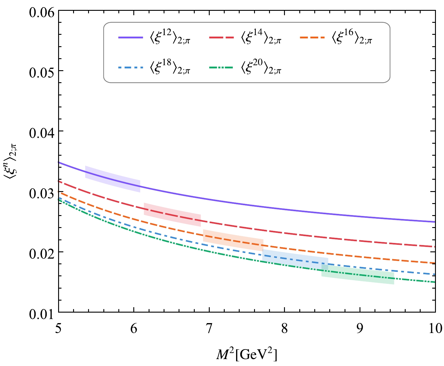
Figure 1. (color online) Pionic leading-twist DA moments
$ \langle\xi^n\rangle_{2;\pi} $ with$ n=(12,14,16,18,20) $ versus the Borel parameter$ M^2 $ ; here, all input parameters are set to their central values. The shaded bands indicate the Borel windows for$ n=(12,14,16,18,20) $ .After considering all uncertainty sources, the values of the pionic leading-twist DA ξ-moments
$ \langle\xi^n\rangle_{2;\pi}|_{\mu} $ with$ n=(12,14,16,18,20) $ can be obtained as$ \begin{aligned}[b] \left<\xi^{12}\right>_{2;\pi} =& 0.0408^{+0.0050}_{-0.0049}, \quad \left<\xi^{14}\right>_{2;\pi} = 0.0346^{+0.0045}_{-0.0045}, \\ \left<\xi^{16}\right>_{2;\pi} =& 0.0301^{+0.0042}_{-0.0041}, \quad \left<\xi^{18}\right>_{2;\pi} = 0.0266^{+0.0039}_{-0.0038}, \\ \left<\xi^{20}\right>_{2;\pi} =& 0.0239^{+0.0037}_{-0.0036} \end{aligned} $

(18) on the scale of
$\mu = 1~{\rm GeV}$ .Next, we can fit the values of the ξ-moments listed in Eqs. (16) and (18) with the models introduced in Sec. II by adopting the least squares method. For the specific fitting procedure, readers can refer to Refs. [3, 63]. Based on the brief review on pionic leading-twist DA models such as the TF model, LCHO model, DSE model, AdS/QCD model, and PLP model presented in Sec. II, we first specify the fitting parameters
$ \mathbf{\theta} $ as follows:$ \mathbf{\theta} = (a_2^{2;\pi}) $ ,$ (a_2^{2;\pi}, a_4^{2;\pi}) $ ,$ (\alpha_{2;\pi}, B_2^{2;\pi}) $ ,$ (\alpha^{\rm DSE}, a_2^{\rm DSE}) $ ,$ (\sqrt{\lambda}, \hat{m}_q) $ ,$ (\sqrt{\lambda}, \hat{m}_q) $ , and$ (\alpha) $ for$ \phi_{2;\pi}^{\rm TF,I} $ ,$ \phi_{2;\pi}^{\rm TF,II} $ ,$ \phi_{2;\pi}^{\rm LCHO} $ ,$ \phi_{2;\pi}^{\rm DSE} $ ,$ \phi_{2;\pi}^{\rm AdS,I} $ ,$ \phi_{2;\pi}^{\rm AdS,II} $ , and$ \phi_{2;\pi}^{\rm PLP} $ , respectively.To analyze the constraint strength of the moments on the model, we use the pionic leading-twist DA models introduced in Sec. II to fit the values of the first nonzero three ξ-moments, five ξ-moments, seven ξ-moments, nine ξ-moments, and ten ξ-moments. That is, we set the values of the ξ-moments listed in Eqs. (16) and (18) to the form of the following five groups as the fitting samples:
$ \begin{aligned}[b] {\rm NS}: 3,& \quad \left\{ \left<\xi^2\right>_{2;\pi}, \left<\xi^4\right>_{2;\pi}, \left<\xi^6\right>_{2;\pi} \right\}; \\ {\rm NS}: 5,& \quad \left\{ \left<\xi^2\right>_{2;\pi}, \left<\xi^4\right>_{2;\pi}, \left<\xi^6\right>_{2;\pi}, \left<\xi^8\right>_{2;\pi}, \left<\xi^{10}\right>_{2;\pi} \right\}; \\ {\rm NS}: 7,& \quad \left\{ \left<\xi^2\right>_{2;\pi}, \left<\xi^4\right>_{2;\pi}, \left<\xi^6\right>_{2;\pi}, \left<\xi^8\right>_{2;\pi}, \left<\xi^{10}\right>_{2;\pi}, \left<\xi^{12}\right>_{2;\pi}, \left<\xi^{14}\right>_{2;\pi} \right\}; \\ {\rm NS}: 9,& \quad \left\{ \left<\xi^2\right>_{2;\pi}, \left<\xi^4\right>_{2;\pi}, \left<\xi^6\right>_{2;\pi}, \left<\xi^8\right>_{2;\pi}, \left<\xi^{10}\right>_{2;\pi}, \left<\xi^{12}\right>_{2;\pi}, \left<\xi^{14}\right>_{2;\pi}, \left<\xi^{16}\right>_{2;\pi}, \left<\xi^{18}\right>_{2;\pi} \right\}; \\ {\rm NS}: 10,& \quad \left\{ \left<\xi^2\right>_{2;\pi}, \left<\xi^4\right>_{2;\pi}, \left<\xi^6\right>_{2;\pi}, \left<\xi^8\right>_{2;\pi}, \left<\xi^{10}\right>_{2;\pi}, \left<\xi^{12}\right>_{2;\pi}, \left<\xi^{14}\right>_{2;\pi}, \left<\xi^{16}\right>_{2;\pi}, \left<\xi^{18}\right>_{2;\pi}, \left<\xi^{20}\right>_{2;\pi} \right\}, \end{aligned} $ 
(19) where
$ \rm NS $ is an abbreviation denoting the number of samples.The fitting results are summarized in Table 2, and the corresponding model curves are displayed in Fig. 2. In the fitting process, the errors of the ξ-moments
$ - $ arising from error sources such as the hadron parameters, light quark masses, and vacuum condensates$ - $ are assumed to be variances. One can discuss the uncertainties of the fitted model parameters by setting an appropriate threshold for$ P_{\chi^2} $ , as in Ref. [63]. However, to better analyze the constraint imposed by different numbers of ξ-moments on the different pion DA models, only the optimal fitted results are provided here. From Table 2 and Fig. 2, one can observe the following:Models NS $ 3 $ 

$ 5 $ 

$ 7 $ 

$ 9 $ 

$ 10 $ 

$ \phi_{2;\pi}^{\rm TF,I} $ 

$ a_2^{2;\pi} $ 

$ 0.225 $ 

$ 0.247 $ 

$ 0.268 $ 

$ 0.285 $ 

$ 0.293 $ 

$ \chi^2_{\rm min} $ 

$ 0.565723 $ 

$ 4.14428 $ 

$ 11.4704 $ 

$ 21.9983 $ 

$ 28.1611 $ 

$ P_{\chi^2_{\rm min}} $ 

$ 0.753624 $ 

$ 0.386832 $ 

$ 0.0748825 $ 

$ 0.00491901 $ 

$ 0.000896493 $ 

$ \phi_{2;\pi}^{\rm TF,II} $ 

$ a_2^{2;\pi} $ 

$ 0.205 $ 

$ 0.197 $ 

$ 0.187 $ 

$ 0.177 $ 

$ 0.172 $ 

$ a_4^{2;\pi} $ 

$ 0.060 $ 

$ 0.098 $ 

$ 0.131 $ 

$ 0.158 $ 

$ 0.170 $ 

$ \chi^2_{\rm min} $ 

$ 0.0162808 $ 

$ 0.480741 $ 

$ 1.6772 $ 

$ 3.78499 $ 

$ 5.17049 $ 

$ P_{\chi^2_{\rm min}} $ 

$ 0.898467 $ 

$ 0.923102 $ 

$ 0.891759 $ 

$ 0.804182 $ 

$ 0.739208 $ 

$ \phi_{2;\pi}^{\rm LCHO} $ 

$ A_{2;\pi} $ 

$ 5.61391 $ 

$ 6.6104 $ 

$ 8.78724 $ 

$ 8.78198 $ 

$ 8.90258 $ 

$ \alpha_{2;\pi} $ 

$ -0.789 $ 

$ -0.684 $ 

$ -0.504 $ 

$ -0.504 $ 

$ -0.493 $ 

$ B_2^{2;\pi} $ 

$ -0.163 $ 

$ -0.155 $ 

$ -0.136 $ 

$ -0.135 $ 

$ -0.133 $ 

$ \beta_{2;\pi} $ 

$ 1.56878 $ 

$ 1.60137 $ 

$ 1.61753 $ 

$ 1.62474 $ 

$ 1.62855 $ 

$ \chi^2_{\rm min} $ 

$ 0.0522982 $ 

$ 0.188917 $ 

$ 0.478592 $ 

$ 1.0968 $ 

$ 1.53822 $ 

$ P_{\chi^2_{\rm min}} $ 

$ 0.819111 $ 

$ 0.979358 $ 

$ 0.992886 $ 

$ 0.993112 $ 

$ 0.992055 $ 

$ \phi_{2;\pi}^{\rm DSE} $ 

$ \alpha^{\rm DSE} $ 

$ 1.130 $ 

$ 0.948 $ 

$ 0.829 $ 

$ 0.738 $ 

$ 0.703 $ 

$ a_2^{\rm DSE} $ 

$ 0.129 $ 

$ 0.048 $ 

$ -0.035 $ 

$ -0.124 $ 

$ -0.166 $ 

$ \chi^2_{\rm min} $ 

$ 0.00559501 $ 

$ 0.174471 $ 

$ 0.422942 $ 

$ 0.694404 $ 

$ 0.818127 $ 

$ P_{\chi^2_{\rm min}} $ 

$ 0.940374 $ 

$ 0.981061 $ 

$ 0.994674 $ 

$ 0.998378 $ 

$ 0.999157 $ 

$ \phi_{2;\pi}^{\rm AdS,I} $ 

$ N_1 $ 

$ 6.24998 $ 

$ 5.58365 $ 

$ 7.40491 $ 

$ 4.99094 $ 

$ 8.06215 $ 

$ \sqrt{\lambda} $ 

$ 0.319 $ 

$ 0.344 $ 

$ 0.305 $ 

$ 0.379 $ 

$ 0.301 $ 

$ \hat{m}_q $ 

$ 0.076 $ 

$ 0.077 $ 

$ 0.064 $ 

$ 0.075 $ 

$ 0.058 $ 

$ \chi^2_{\rm min} $ 

$ 0.0395365 $ 

$ 1.13085 $ 

$ 3.82526 $ 

$ 7.94241 $ 

$ 10.3942 $ 

$ P_{\chi^2_{\rm min}} $ 

$ 0.84239 $ 

$ 0.769632 $ 

$ 0.574839 $ 

$ 0.3377 $ 

$ 0.238443 $ 

$ \phi_{2;\pi}^{\rm AdS,II} $ 

$ N_2 $ 

$ 0.443594 $ 

$ 0.405197 $ 

$ 0.399993 $ 

$ 0.395313 $ 

$ 0.392851 $ 

$ \sqrt{\lambda} $ 

$ 1.342 $ 

$ 1.212 $ 

$ 1.248 $ 

$ 1.286 $ 

$ 1.300 $ 

$ \hat{m}_q $ 

$ 0.042 $ 

$ 0.084 $ 

$ 0.082 $ 

$ 0.080 $ 

$ 0.080 $ 

$ \chi^2_{\rm min} $ 

$ 0.00512763 $ 

$ 0.256752 $ 

$ 1.20083 $ 

$ 2.9544 $ 

$ 4.08025 $ 

$ P_{\chi^2_{\rm min}} $ 

$ 0.942914 $ 

$ 0.967946 $ 

$ 0.944797 $ 

$ 0.889188 $ 

$ 0.849812 $ 

$ \phi_{2;\pi}^{\rm PLP} $ 

α $ 0.380 $ 

$ 0.379 $ 

$ 0.370 $ 

$ 0.359 $ 

$ 0.354 $ 

$ \chi^2_{\rm min} $ 

$ 0.199311 $ 

$ 0.219225 $ 

$ 0.452207 $ 

$ 1.04863 $ 

$ 1.46392 $ 

$ P_{\chi^2_{\rm min}} $ 

$ 0.905149 $ 

$ 0.994414 $ 

$ 0.998372 $ 

$ 0.997922 $ 

$ 0.997406 $ 

Table 2. Fitting results for different DA models obtained by fitting the values of the first several nonzero pionic leading-twist DA ξ-moments listed in Eqs. (16) and (18) via the least squares method.
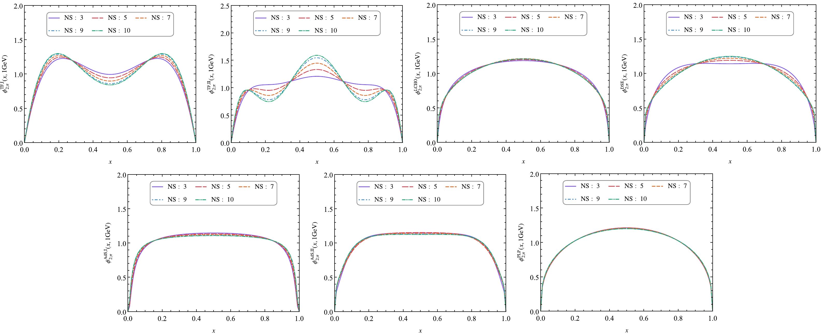
Figure 2. (color online) Curves of pionic leading-twist DA models such as the TF model, LCHO model, DSE model, AdS/QCD model, and PLP model corresponding to the fitting results presented in Table 2.
● At
$ {\rm NS} = 10 $ ,$ P_{\chi^2_{\rm min}} $ for$ \phi_{2;\pi}^{\rm TF,I} $ and$ \phi_{2;\pi}^{\rm AdS,I} $ is far less than$ 1 $ ,$ P_{\chi^2_{\rm min}} \simeq 0.74 $ for$ \phi_{2;\pi}^{\rm TF,II} $ , and$ P_{\chi^2_{\rm min}} \simeq 0.85 $ for$ \phi_{2;\pi}^{\rm AdS,II} $ ; however,$ P_{\chi^2_{\rm min}} > 0.99 $ and is very close to$ 1 $ for$ \phi_{2;\pi}^{\rm LCHO} $ ,$ \phi_{2;\pi}^{\rm DSE} $ , and$ \phi_{2;\pi}^{\rm PLP} $ . This indicates that the results of the LCHO model, DSE model, and PLP model are very consistent with our values for the first ten nonzero ξ-moments listed in Eqs. (16) and (18) obtained based on the QCD sum rules.● The goodness of fits for the models
$ \phi_{2;\pi}^{\rm TF,I} $ and$ \phi_{2;\pi}^{\rm AdS,I} $ decrease with increasing NS, whereas the goodness of fits for the models$ \phi_{2;\pi}^{\rm LCHO} $ ,$ \phi_{2;\pi}^{\rm DSE} $ , and$ \phi_{2;\pi}^{\rm PLP} $ are very close to each other for different NS. This indicates that more numerous moments impose stronger constraints on the DA behavior. Thus, adequate moments can easily help us eliminate inappropriate models and select an appropriate model to better describe the correct DA behavior.● The goodness of fit for model
$ \phi_{2;\pi}^{\rm AdS,II} $ is better than that for$ \phi_{2;\pi}^{\rm AdS,I} $ under$ {\rm NS} = 3,5,7,9,10 $ . This indicates that$ \phi_{2;\pi}^{\rm AdS,II} $ based on a consideration of the influence of the Dirac structure$ \not p\gamma_5 $ on the WF is more consistent with our sum rule results for ξ-moments. However, by fitting the first ten nonzero ξ-moments with$ \phi_{2;\pi}^{\rm AdS,II} $ , we obtain the following model parameters:$ \sqrt{\lambda} = 1.300~ {\rm GeV} $ and$ \hat{m}_q = 80~ {\rm MeV} $ . The obtained value of$ \sqrt{\lambda} $ is much greater than that reported in the literature. The obtained value of$ \hat{m}_q $ is consistent with the value obtained by fitting the pion and kaon decay constants in Ref. [13]; however, it is larger than the value obtained by fitting the Regge trajectories of pseudoscalar mesons in Ref. [72].● The curves of
$ \phi_{2;\pi}^{\rm TF,I} $ and$ \phi_{2;\pi}^{\rm TF,II} $ with different NS are significantly different from each other. This implies that models$ \phi_{2;\pi}^{\rm TF,I} $ and$ \phi_{2;\pi}^{\rm TF,II} $ are far from being enough to describe the behavior of the pionic leading-twist DA. Therefore, the DAs obtained by calculating the second and/or fourth Gegenbauer moments using LQCD or QCD sum rules and substituting them into$ \phi_{2;\pi}^{\rm TF,I} $ and$ \phi_{2;\pi}^{\rm TF,II} $ in Eqs. (2) and (3) are also far from being adequate to describe the behavior of the pionic leading-twist DA. However, the goodness of fit of$ \phi_{2;\pi}^{\rm TF,II} $ is better than that of$ \phi_{2;\pi}^{\rm TF,I} $ with the same NS. This indicates that by increasing the number of terms in the TF, i.e., N in Eq. (1), the ability of the TF model to describe the behavior of the pionic leading-twist DA can be improved.● The curves of
$ \phi_{2;\pi}^{\rm LCHO} $ with$ {\rm NS = 3,5,7,9,10} $ almost coincide with each other; the same results are observed for$ \phi_{2;\pi}^{\rm AdS,I} $ ,$ \phi_{2;\pi}^{\rm AdS,II} $ , and$ \phi_{2;\pi}^{\rm PLP} $ . This indicates that the LCHO model, AdS/QCD model, and PLP model present strong prediction abilities for the behavior of the pionic leading-twist DA. The three models obtained by using the first few Gegenbauer moments or ξ -moments to constrain the model parameters are adequate to describe the behavior of the pionic leading-twist DA. However, from the goodness of fits for$ \phi_{2;\pi}^{\rm AdS,I} $ and$ \phi_{2;\pi}^{\rm AdS,II} $ summarized in Table 2, one can find that these two models are not very consistent with our QCD sum rule results. -
In this paper, we calculate the pionic leading-twist DA ξ-moments
$ \left<\xi^n\right>_{2;\pi}(n = 12,14,16,18,20) $ using the sum rule formula for the nth ξ-moment, Eq. (13), suggested in our previous study [3]. In this calculation, the contributions from the continuum state and dimension-six condensate are less than$ 40 $ % and$ 5 $ % for the obtained five ξ-moments. Owing to the form of the sum rules in Eq. (13), the limitation of the system error, which results from the missing higher-dimension condensates and the continuum and excited states under the quark-hadron duality approximation, on the prediction ability of the QCD sum rule method for higher-order ξ-moments is alleviated. The values of the ξ-moments$ \left<\xi^n\right>_{2;\pi}(n = 12,14,16, 18,20) $ are hence reliable and are listed in Eq. (18). By combining the values of$ \left<\xi^n\right>_{2;\pi}(n = 2,4,6,8,10) $ calculated in our previous study [3] and considering the values of the first ten nonzero ξ-moments as samples, we analyze several common and relatively simple models of the pionic leading-twist DA, including the TF model, LCHO model, DSE model, AdS/QCD model, and PLP model, based on the least squares method. Consequently, we find that the TF model is not sufficient to describe the behavior of the pionic leading-twist DA. By contrast, the LCHO model, AdS/QCD model, and PLP model have strong prediction abilities for the pionic leading-twist DA. The results of the LCHO model, DSE model, and PLP model are extremely consistent with our values for the first ten nonzero ξ-moments listed in Eqs. (16) and (18) obtained based on the QCD sum rules.The relevant literature contains several calculation approaches for the ξ-moments and Gegenbauer moments of the pionic leading-twist DA. However, most of the associated studies only focus on the lowest order. Our numerical analysis reveals that only the lowest order moment is far from being enough to determine the overall behavior of the DA. Therefore, we believe that if higher-order and more accurate ξ-moments can be calculated based on new methods, we may be able to judge various phenomenological models more strictly and estimate the behavior of the pionic leading-twist DA more accurately.
-
We are grateful to Professor Qin Chang for helpful discussions and valuable suggestions.
Constraints of ξ-moments computed using QCD sum rules on piondistribution amplitude models
- Received Date: 2022-09-08
- Available Online: 2023-01-15
Abstract: To date, the behavior of the pionic leading-twist distribution amplitude (DA)


 DownLoad: