Globally Stable Dark Energy in F(R) Gravity

Since the discovery of the current acceleration of the cosmic expansion about a quarter-century ago [1, 2], numerous attempts have been made to explain the underlying repulsive energy source, referred to as dark energy [3−6]. In addition to the static cosmological constant [7−9], dark energy could also be attributed to a dynamical scalar field emerging, for instance, from $ F(R) $ gravity [10−12]. By replacing the Ricci scalar R with a general function $ F(R) $, $ F(R) $ gravity introduces an additional scalar degree of freedom, dubbed scalaron.

Capozziello was the first to explore cosmic acceleration within the framework of $ F(R) $ gravity by incorporating quintessence, called curvature quintessence [13]. Subsequently, Carroll et al. proposed the first well-studied model [14], while Nojiri et al. proposed the first potential unified model to describe both primordial and late-time acceleration within a single $ F(R) $ Lagrangian [15]. Such a light scalar field would mediate a long-range fifth force, which is tightly constrained by solar-system tests through the Parameterized Post-Newtonian (PPN) parameter. Fortunately, nonlinear effects can screen the propagation of the fifth force via the chameleon mechanism [16−18]. After a few years of exploration, several viable models have been successfully developed [19−23].

However, it was soon recognized that these models typically lead to a weak curvature singularity, occurring in the past [20, 22, 24, 25] (for discussions on finite-time singularities, see [26−29]). As a result, the scalaron mass exceeds the Planck mass even during the matter-dominated era, signaling the breakdown of $ F(R) $ gravity as an effective field theory. It has been found that adding an $ R^2 $ term can naturally remove the singularity, and the resulting $ R^2 $-corrected dark energy may provide a unified description of primordial and late-time acceleration of the cosmic expansion [30−33]. For general considerations or related work, see Refs. [34−41].

In such a unified scenario, the standard sequence of inflation, reheating, radiation-dominated, matter-dominated, and dark energy-dominated epochs must be preserved. In the original $ R^2 $ inflationary model, post-inflationary reheating begins when the linear R term dominates over the nonlinear $ R^2 $ term and oscillates around the vacuum state $ R=0 $. Adhering to this reheating mechanism suggests that not all viable dark energy models can fulfill these criteria, as many become unstable when $ R<0 $. The only viable model, to the best of my knowledge, is the Appleby-Battye model [31], which, unlike others, was specifically designed with the condition $ F_R>0 $ for all ranges of Ricci scalar [21]. For recent cosmological constraints, see [42].

In this paper, we will generalize the idea from the Appleby-Battye model and demonstrate that the favored form of $ F_R(R) $ is a bounded function with a sigmoid shape, with its midpoint (or center of symmetry) determined by the critical curvature. In addition, the ΛCDM model (for positive R) can be regarded as an extreme case of these sigmoid functions, i.e., the Heaviside delta function of R.

The Appleby-Battye model contains exponential terms, and as we will show, the first derivative is actually the logistic function. For comparison, we will also introduce a new model whose first derivative approximates a power-law behavior in the high-curvature limit. Consequently, our model resembles the well-studied Hu-Sawicki model in the high-curvature limit but achieves global stability. We demonstrate that this model can account for the current cosmic acceleration by explicitly solving the Friedmann equation. Furthermore, the effective Equation of State (EoS) parameter for the dark energy component exhibits phantom crossing behavior, a common feature of $ F(R) $ dark energy models [43−45]. Next, We constrain the model parameters by confronting our model with local gravity tests. Finally, We discuss the unified description of dark energy and inflation within the framework of globally stable models.

Throughout this paper, we adopt natural units with $ c=\hbar=1 $ and focus exclusively on the metric formalism, where the metric signature is $ (-,+,+,+) $. A prime "$ \prime $" and a subscript "R" denote derivatives with respect to the function's argument and Ricci scalar, respectively.

The action of $ F(R) $ gravity is given by

where $ \kappa^{2}\equiv8\pi G\equiv1/M_{\mathrm{Pl}}^{2} $ with G being the bare gravitational constant and $ M_{\mathrm{Pl}}\simeq 2.44\times10^{18}\,\mathrm{GeV} $ being the reduced Planck mass, $ S_{\mathrm{Matter}} $ is the matter action describing all non-gravitational parts. For convenience, we define $ F(R)\equiv R+f(R) $, such that the modification to the general relativity is encoded in $ f(R) $.

Variation with respect to the metric $ g^{\mu\nu} $ gives the modified field equation,

where $ F_{R}\equiv\partial F/\partial R $. The trace of the field equation (2) reads

indicating a propagating scalar degree of freedom, $ f_{R} $, dubbed scalaron. The dynamics of the scalaron is subject to an effective potential $ U_{\mathrm{eff}} $:

The mass squared of the scalaron at the extremum $ \dfrac{\partial U_{\mathrm{eff}}}{\partial f_{R}}=0 $ is defined by

On the other hand, the vacuum solutions can be determined from

Especially we have $ R=4\Lambda $ in the ΛCDM model. If the solution satisfies

then the de sitter point is future-stable with the mass squared being positive.

We can rewrite the action in the form of scalar-tensor theories by introducing an auxiliary field χ:

Variation of the action with respect to χ yields

If $ F_{,\chi\chi} $ is not identically vanishing, then $ \chi=R $. Therefore, we can define

such that

Since the field equation (3) is a fourth-order differential equation of $ g_{\mu\nu} $, an intuitive way is to transform the action into the Einstein frame through the Weyl transformation:

where β is the coupling constant, and φ is a new scalar field defined in the Einstein frame:

Choosing $ \beta=-\dfrac{1}{\sqrt{6}} $, the action is rewritten as the Einstein-Hilbert term plus a canonical scalar field:

where, $ V(\varphi) $ is the potential of the scalaron given by

In the Einstein frame, the scalaron is non-minimally coupled to the matter fields, and the energy-momentum tensor of matter fields is

So does the energy density $ \tilde{\rho}=e^{4\beta\kappa\varphi}\rho $ and pressure $ \tilde{P}=e^{4\beta\kappa\varphi}P $. Since $ w=P/\rho $, the EoS parameter is independent of frame transformation. On the other hand, the conserved energy density in the Einstein frame is

rather than $ \tilde{\rho} $. For dust-like matter $ w=0 $, $ \tilde{\rho}_{*}=e^{3\beta\kappa\varphi}\rho $; for radiation, $ w=1/3 $, $ \tilde{\rho}_{*}=e^{4\beta\kappa\varphi}\rho=\tilde{\rho} $.

The equation of motion for the scalaron is

Thus, the scalaron is subject to an effective potential:

so, the effective mass squared is defined by $ m_{\varphi}^{2}\equiv V_{\mathrm{eff},\varphi\varphi}(\varphi_{\min}) $, where $ \varphi_{\mathrm{min}} $ is the equilibrium value corresponding to the minimum of the effective potential, which is determined by the trace $ T_{\mu}^{\mu} $.

Generally speaking, a cosmologically viable model for dark energy in $ F(R) $ gravity should at least satisfy the following viability conditions [31, 43]:

where $ R_{1} $ be the maximal de sitter solution. The first condition is imposed to evade anti-gravity and ghost state of the graviton [31, 46, 47] and the second condition ensures the mass squared to be positive and avoid Dolgov-Kawasaki instability and Tachyon instability [31, 48−51]. Other viable conditions can be inferred from dynamical analysis [43]. To be distinguished with ΛCDM model, it is suggested that $ F(R) $ gravity does not contain true cosmological constant, i.e., $ F(0)=0 $ [20].

The above conditions impose stringent constraints on possible forms of the $ F(R) $ function.

Some well-studied viable models satisfying the above requirements are (with different notations to the original papers):

● Hu-Sawicki model [19]

where, $ c_{1},c_{2}>0 $ are free parameters. $ R_{\mathrm{c}}\equiv\dfrac{\kappa^{2}\bar{\rho}_{\mathrm{m}0}}{3} $, where $ \bar{\rho}_{\mathrm{m}0}=\bar{\rho}_{\mathrm{m}}(\ln a=0) $ is the averaged matter density today.

● Starobinsky model [20]

where, $ n,\lambda>0 $, $ R_\mathrm{c} $ is the order of the observed cosmological constant $ \Lambda\simeq10^{-66}\,\mathrm{eV^{2}} $.

● Tsujikawa model [22]

where, $ \lambda,b>0 $.

● Exponential model [23]

where, $ \lambda, b>0 $.

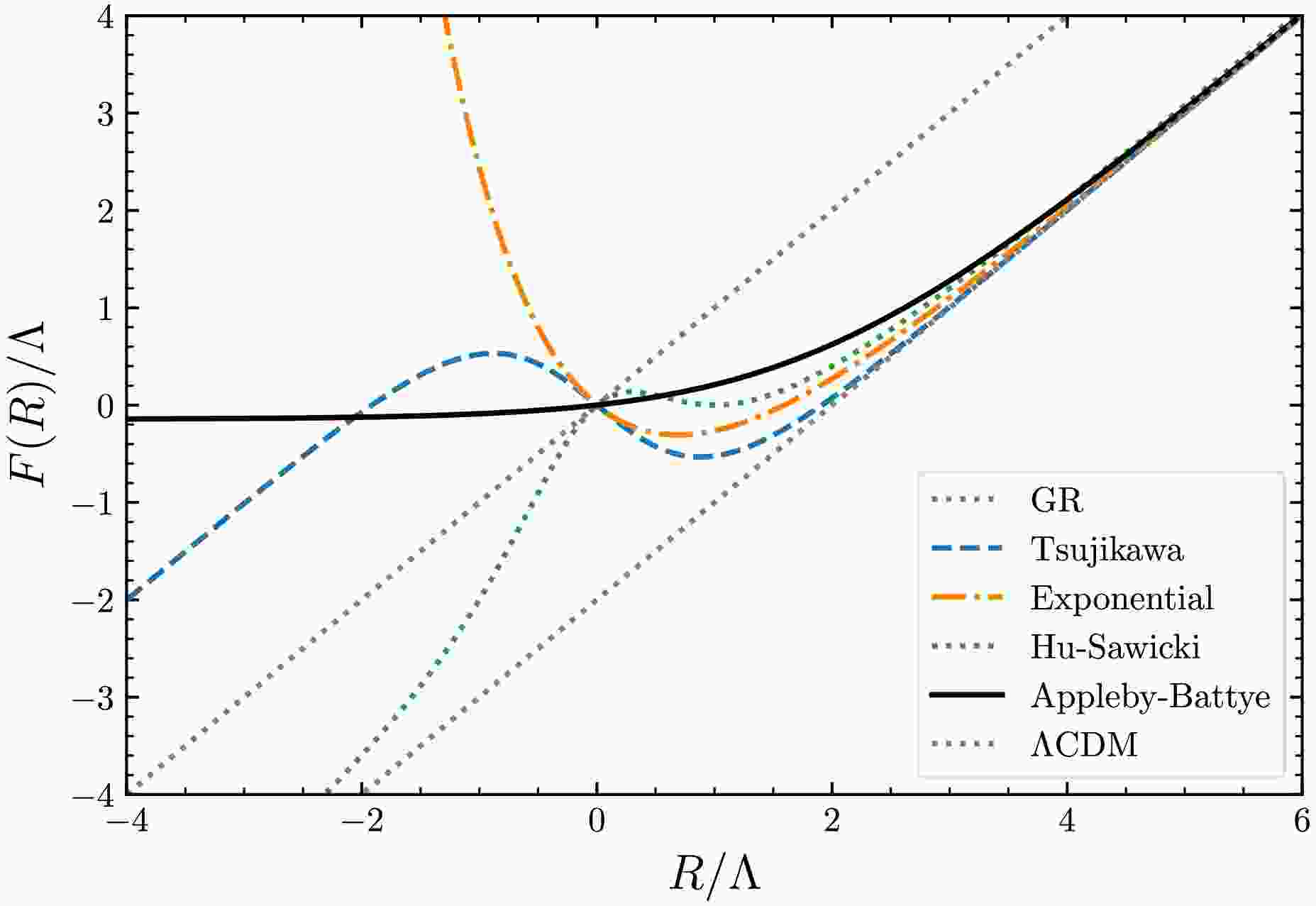
These models are carefully constructed by requiring the $ F(R) $ to satisfy the viability conditions. Physically, it is required that $ |F(R)-R|\ll R $, $ F_{R}-R\ll 1 $, and $ RF_{RR}\ll 1 $ for $ R\gg R_{0}=R(t_0) $ to preserve the success of general relativity [31]. Practically, as shown in Fig. 1, all models listed above approximate to $ F(R)\approx R-\lambda R_\mathrm{c}+\cdots $ in the high-curvature limit. Therefore, $ \lambda R_\mathrm{c} $ can be interpreted as $ 2\Lambda $. Although it is claimed that there is no true cosmological constant in $ F(R) $ gravity if we impose $ F(0)=0 $, it effectively introduces a cosmological constant in the Lagrangian. Mathematically, this is because one has to introduce a critical curvature $ R_\mathrm{c} $ to ensure a correct normalized argument, $ R/R_\mathrm{c} $, in the nonlinear function $ f(R) $. It leads to different asymptotic behaviors in various limits, with $ F(R\gg R_\mathrm{c})\to R-\lambda R_\mathrm{c} $ in the high-curvature limit. In this work, we adopt the asymptotic behavior as a constraint for parameterizing models while acknowledging that some alternative models may not satisfy this condition. It is important to note, however, that this behavior is not a necessary condition for our model-building process.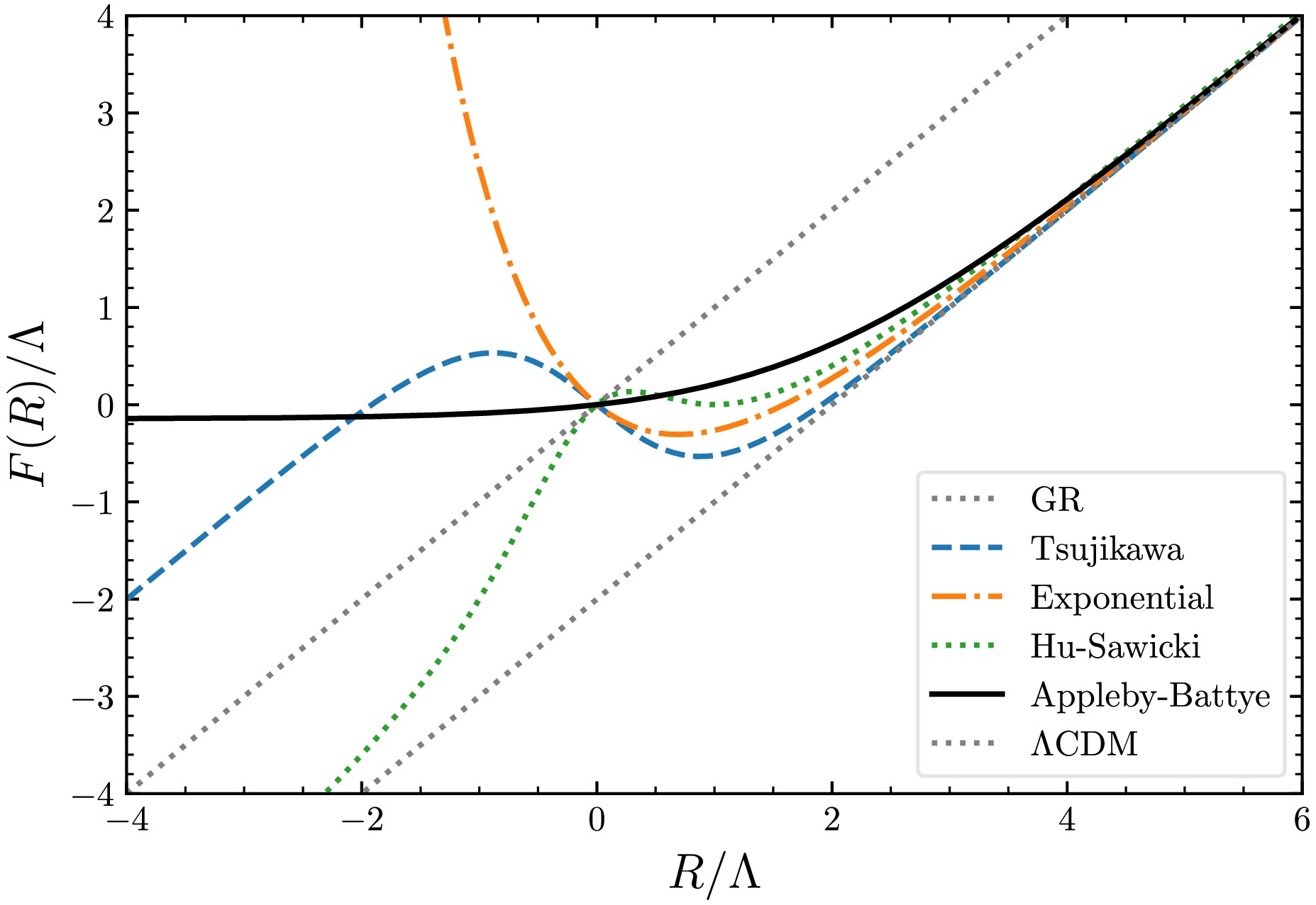

Figure 1.  (color online) Comparison of $ F(R)/\Lambda $ versus $ R/\Lambda $ for existing models, with all parameters set to unity. The Starobinsky model is not shown here, as it coincides with the Hu-Sawicki model for $ n=1 $.

As shown in Fig. 2, one also notes that $ F_R $ and $ F_{RR} $ become negative when $ R \sim 0 $ for most models listed above. Although this does not pose an immediate issue since $ R \sim 0 $ is generally inaccessible in redthe current universe, it introduces challenges when attempting to build a unified model by adding an $ R^2 $ term to the $ F(R) $ Lagrangian to explain both primordial and late-time cosmic acceleration. Specifically, in the original $ R^2 $ inflation scenario, efficient reheating necessitates an oscillating R around the vacuum state $ R = 0 $. Consequently, for model stability, it is essential that $ F_{R} > 0 $ and $ F_{RR} > 0 $ hold within the accessible negative R region. Otherwise, for instance, if $ F_{RR} < 0 $, the vacuum state becomes unstable, and the scalaron mass diverges when $ F_{RR} = 0 $ [11].

Figure 2.  (color online) Comparison of $ F_{R}(R) $ (left panel) and $ \Lambda F_{RR}(R) $ (right panel) versus $ R/\Lambda $ for existing models, with all parameters set to unity.

On the other hand, the Appleby-Battye model (the black solid line in Fig. 2) has no such problem since it was constructed by initially imposing $ F_R>0 $ for all R [21]. The advantage of constructing models starting from $ F_{R}(R) $ rather than $ F(R) $ is that it is easier to ensure $ F_{R}>0 $ and $ F_{RR}>0 $ for all R. However, the disadvantage is that it is not always straightforward to explicitly derive the primitive $ F(R) $ function by integrating the given $ F_{R} $ function. $ F_{RR}>0 $ means that $ F_{R} $ should be monotonically increasing. In addition, $ F_{R}>0 $ and $ F(R\gg R_\mathrm{c})\to R-2\Lambda $ require that it is a bounded function, $ 0<F_{R}<1 $ [21]. The first derivative of the Appleby-Battye model (27) was chosen as [21]

where a and b are free parameters. The resulting $ F(R) $ model reads [21]

The other form often seen in the literature is written as [31]

where $ \epsilon_{\mathrm{AB}}=R_{\mathrm{vac}}/\left(b+\ln(2\cosh b)\right) $, with b being the model parameter and $ R_{\mathrm{vac}}\sim 4\Lambda $ being the vacuum curvature.

Obviously, Eq. (26) is not the only choice that satisfies $ 0<F_R<1 $ and $ F_{RR}>0 $ for all R. To facilitate finding the primitive function for a given $ F_{R}(R) $, we suggest that the desired $ F_{R}(R) $ function should adopt a sigmoid shape, with its midpoint (or center of symmetry) determined by the critical curvature $ R_\mathrm{c} $. Moreover, the interval over which $ F_{R}(R) $ transitions from $ F_{R}(R)=0 $ to $ F_{R}(R)=1 $ should be narrow, enabling $ F_{R}(R) $ to approach the ΛCDM limit rapidly; here, (the positive part of) the ΛCDM is regarded as an extreme case of the sigmoid function, i.e., the Heaviside delta function. Then, the $ F(R) $ model can be derived by integrating the given $ F_{R} $ function and fixing the integration constant through the condition $ F(0)=0 $. As examples, we shall first reformulate the original Appleby-Battye model (27) to show the exponential suppressed term explicitly. Then, we propose a new model whose first derivative exhibits a power-law behavior in the high-curvature limit.

We note that the function (26) is indeed the well-known logistic function:

where L is the maximum, k controls the growth rate or the curve's steepness, and $ x_{0} $ is the midpoint. Analogously, the suggested form of $ F_{R} $ function is

One notes that the midpoint is $ \left(R_{\mathrm{c}}\ln b,\dfrac{1}{2}\right) $, where the parameter b controls the shift of the midpoint, and the curvature scale $ R_{\mathrm{c}} $ controls the steepness of the curve or the clockwise rotation with respect to the midpoint. Specifically, the larger $ R_{\mathrm{c}} $ is, the shallower the curve becomes; conversely, the smaller $ R_{\mathrm{c}} $ is, the steeper the curve is, and the closer the function to the ΛCDM model with $ F_{R}=1 $.

Integrating $ F_R(R) $ with respect to R yields the primitive function,

where C is an integration constant. It can be fixed by imposing $ F(0)=0 $, such that

Then, the full $ F(R) $ function reads

In the high-curvature limit, we have

To mimic the ΛCDM model in the high-curvature limit, we require that $ \lambda R_{\mathrm{c}}=2\Lambda $, with λ defined by

The resulting $ F(R) $ model is then

To quantify how it deviates from the ΛCDM model, we further parameterize the model as

where $ \xi\equiv 2/\lambda=R_{\mathrm{c}}/\Lambda $ characterizes the relative size of $ R_\mathrm{c} $ with respect to Λ. One finds that ξ controls the curve's steepness: the smaller ξ is, the steeper the function is, and the closer the $ F(R) $ model to the ΛCDM model. When $ \xi=0 $, the $ F_R $ becomes a Heaviside delta function at $ R=0 $, and the model recovers the ΛCDM model (for $ R>0 $). For fixed curvature, the model approximates as follows:

We see that the new form (36) provides an alternative understanding of how each parameter and each term works. Furthermore, one can see how it differs from the Tsujikawa and exponential models, which also contain exponential terms. We find that the key point of Eq. (36) to guarantee $ F_{R}>0 $ and $ F_{RR}>0 $ for $ R<0 $ is that the nonlinear term in Eq. (36) is indeed "linearized" when $ R\ll -R_\mathrm{c} $; this results in an absolute Ricci scalar $ |R| $, which is canceled by the linear term R.

The generalization of model (30) is straightforward:

where $ b,n>0 $. It is positive for all R, and its derivative is also positive,

One finds that $ F_{R}(R) $ and $ F_{R}(RR) $ decrease faster as n increases.

Integrating Eq. (39) yields

where, C is an integration constant and $ \,_{2}F_{1}\left(1,1;n+1;-\dfrac{e^{x}}{b}\right) $ is hypergeometric function. It has simple form if $ n\in \mathbb{Z} $; for instance, when $ n=2 $, we have

where the condition $ F(0)=0 $ has been applied to eliminate the integration constant. Further exploration of the generalized model is left for future work.

Having shown the benefit of the sigmoid $ F_{R} $ function and reproduced the original Appleby-Battye model, we now consider models that exhibit a power-law behavior in the high-curvature limit. A simple sigmoid $ F_{R} $ function is

where $ b,c $ are free parameters and $ R_{\mathrm{c}} $ is the critical curvature. It is required that $ c>0 $ for model stability, and we impose that $ R_{\mathrm{c}}>0 $ with b unconstrained.

The midpoint of the function is $ \left(bR_{\mathrm{c}}, \dfrac{1}{2}\right) $. For fixed curvature $ R_{\mathrm{c}} $, b controls the shift of the midpoint and c controls the clockwise rotation: the smaller c is, the steeper the curve becomes, and the closer the model is to the ΛCDM model. When $ c=0 $, it becomes a Heaviside delta function:

Therefore, $ F(R) $ model is indistinguishable with ΛCDM model when $ c=0 $ and $ R>bR_{\mathrm{c}} $.

Integrating $ F_{R}(R) $ yields the primitive function

where C is an integration constant, which can be determined by imposing $ F(0)=0 $:

Then, the full $ F(R) $ function reads

In the high-curvature limit,

To mimic the ΛCDM model, we impose $ \lambda R_{\mathrm{c}}=2\Lambda $, with λ defined by

Since $ c,\lambda>0 $, the parameter b is constrained to be

Therefore, the alternative form is

One observes that, when $ R/R_{\mathrm{c}}\gg b $, the above equation reduces to $ F(R)=R-2\Lambda $. On the other hand, the relation $ R>\lambda R_{\mathrm{c}}>bR_{\mathrm{c}} $ gives the following asymptotic behaviors:

It seems that b can well describe the deviation of this model with respect to the ΛCDM model. Therefore, we can parameterize the model by defining a dimensionless parameter

Then, the model becomes

It has the following asymptotic behaviors:

The allowed parameter space of ξ is $ 0<\xi<+\infty $, while observational constraints suggest $ \xi\ll1 $. Furthermore, we find that b and c are not entirely independent according to the definition of ξ. Following Ref. [19], one can fix $ R_{\mathrm{c}}\equiv\dfrac{8\pi G}{3}\rho_{\mathrm{m}} $, such that the physical density parameter inferred from the ΛCDM model applies to $ F(R) $ models as well. With $ R_\mathrm{c} $ determined, once ξ is known from the observation, other parameters are also determined, $ \xi\rightarrow b\rightarrow \lambda\rightarrow c $. Therefore, our model has only one additional free parameter compared with the ΛCDM model. Moreover, $ \xi\ll1 $ means that $ b\to\lambda $ and $ c\ll4\lambda^{2} $.

Finally, the generalization of this model to higher powers is straightforward:

where C is a constant. Imposing $ F(0)=0 $, we have

Then, the full function reads

In the high-curvature limit,

We require $ \lambda R=2\Lambda $, with λ defined by

Since $ c,\lambda>0 $, the parameter b is confined to

Therefore, the alternative $ F(R) $ form reads

Likewise, by defining $ \xi\equiv1-\dfrac{b}{\lambda} $, the model can be parameterized as

For later convenience, we define $ x\equiv R/\Lambda $ and rewrite the model as following dimensionless forms:

One can readily observe that $ F_{RR}>0 $ if $ n>0.5 $, and the $ F_{R}(R) $ function satisfies

In the high-curvature limit, Eqs. (64) approximate to (up to first order of ξ)

Note that the ξs in the two classes of models have different meanings. In the Appleby-Battye model, $ \xi\equiv\dfrac{2}{\lambda}=\dfrac{R_{\mathrm{c}}}{\Lambda} $, measuring the relative size of the critical curvature with respect to the cosmological constant, whereas in our model,

measuring the relative difference of $ b R_{\mathrm{c}} $ with respect to $ 2\Lambda $. To satisfy the observations, therefore, $ \xi\ll 1 $ in our model, while $ \xi<1 $ in the Appleby-Battye model. It is known that the potential for most of $ F(R) $ dark energy models are multi-valued, and only the branch corresponding to $ F_{R}>0 $ is physical. Using the Hu-Sawicki model as an example, we observe that, as illustrated in the left panel of Fig. 3, only the black sections of the curves are physically relevant. This is not true in globally stable models since $ F_{R}>0 $ for all R. As shown in Fig. 3, the multi-valued nature of the potential naturally disappears in our model. Therefore, the scalar fields defined in both frames exhibit a one-to-one correspondence.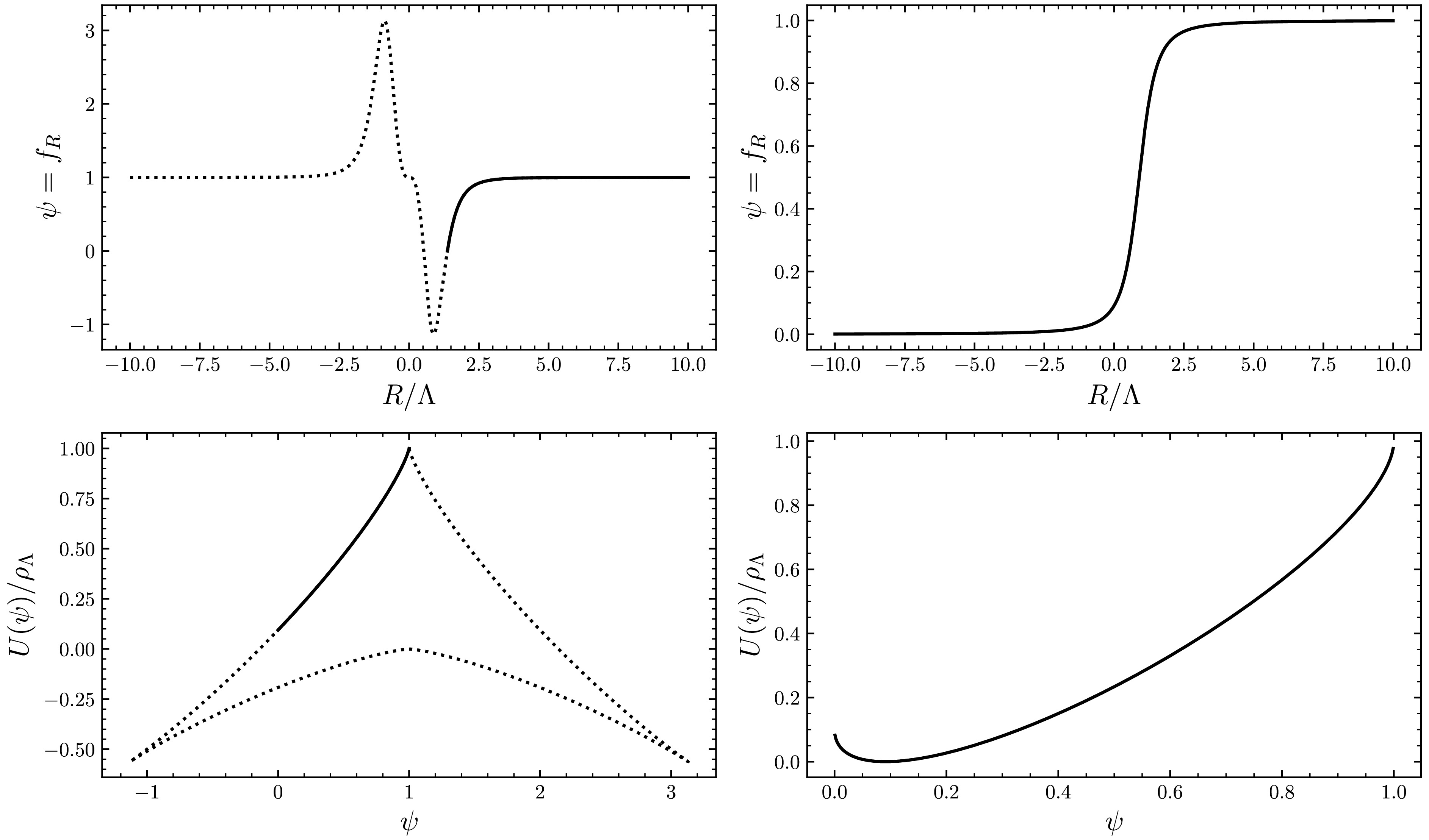

Figure 3.  Comparison of the Jordan-frame field (upper panel) and potential (lower panel) between the Hu-Sawicki model (left panel with $ n=1 $ and $ \xi=0.1 $) and our model (right panel with $ n=1 $ and $ \xi=0.1 $). Here, $ \rho_\Lambda=\frac{\Lambda}{\kappa^2} $.

We now study the cosmological evolution by explicitly solving the Friedmann equation. In the flat Friedmann-Lemaître-Robertson-Walker (FLEW) spacetime, the modified Friedmann equation is

where we have defined an effective energy density rising from modified gravity

Analogously, the modified acceleration equation is

where the effective pressure is

Hence, the effective EoS of the system and dark energy are defined by

and

respectively. Substituting $ \rho\propto a^{-3(1+w)} $ into the Friedmann equation gives

where the density parameter $ \Omega_{i} $ and Hubble parameter $ H_{0} $ are model-dependent, i.e.,

However, their combination, the physical density parameter $ \omega_{i}\equiv\Omega_{i}h^{2} $, is usually model-independent. Therefore,

This relation is convenient when making comparisons.

We now rewrite the equations in a dimensionless form. We first define dimensionless Hubble parameter $ E\equiv H/H_{0}^{\Lambda\mathrm{CDM}} $ (in the following, we neglect notation ΛCDM) and replace the cosmic time t by redshift z. Then, the Friedmann equation becomes

where the subscript ”z” denotes a derivative with respect to z. According to $ f(R) $ and its derivatives, the above three terms, respectively, represent the second-order, first-order, and zeroth-order corrections of the Friedmann equation in $ F(R) $ gravity with respect to the ΛCDM model (with $ f=-2\Lambda $). In addition, we have written all quantities in dimensionless forms, i.e., $ f(R)/\Lambda $, $ f_{R}(R) $ and $ \Lambda f_{RR} $. The Ricci scalar is normalized by

where, $ \Omega_{\Lambda0}=\Lambda/3H_{0}^{2} $.

We assume that the $ F(R) $ model reduces to the ΛCDM model in the high redshift to solve the modified Friedmann equation. Then, the initial conditions can be inferred from the ΛCDM model:

Therefore,

After solving $ E(z) $ and $ E_{z}(z) $, the calculation of the eff EoS for the system and the dark energy component is straightforward:

Note that the density parameters used here are those from the ΛCDM model. The resulting Hubble constant and density parameter are

Substituting our model into Eq. (77), we can extract the Hubble parameter and EoS. As shown in Fig. 4, the Hubble parameter in $ F(R) $ deviates from that in ΛCDM model when $ z<2 $, resulting in a slightly larger Hubble constant. Figure 5 compares the differences in EoS between the two models. We find that the two models exhibit a similar evolution of the EoS for the system; however, the EoS for the dark energy component shows significant differences: there is a phantom crossing in our model when $ z<4 $ (with initial values chosen above). This behavior is a universal characteristic of $ F(R) $ dark energy models [19, 44, 52−55]. Therefore, our model can be distinguished from the ΛCDM model.

Figure 4.  (color online) Hubble parameter H as a function of $ 1+z $, with $ n=2.5 $ and $ \xi=0.01 $. The lower panel shows the relative difference $ \frac{H(z)-H^{\Lambda\mathrm{CDM}}(z)}{H^{\Lambda\mathrm{CDM}}(z)} $.

Figure 5.  (color online) Comparison of the EoS parameter between our model and the ΛCDM model, with $ n=2.5 $ and $ \xi=0.01 $. The upper and lower panels display the effective EoS for dark energy, $ w_{\mathrm{de}} $, and the effective EoS for the entire system, $ w_{\mathrm{eff}} $, respectively.

In this section, we confront our model with local gravity tests. The calculation details refer to Refs. [11, 16, 17, 56, 57]. For the latest reviews on chameleons, see [58, 59].

In the Einstein frame, the scalaron couples to the trace of energy-momentum tensor matter with a universal coupling constant $ \beta=-1/\sqrt{6} $. In the dense region, we have $ T_{\mu}^{\mu}\approx-\rho_{\mathrm{m}} $. We consider a spherical static body with radius $ \tilde{r}_{\mathrm{c}} $, in which case the background spacetime is approximated to the Minkowski one. Variation with respect to Eq. (15) yields

where the effective potential is

$ \tilde{\rho}_{*} $ is the conserved energy density in the Einstein frame (18) satisfying $ \tilde{r}^{3}\tilde{\rho}_{*}=r^{3}\rho $. For given mass density $ \tilde{\rho}_{*} $, the effective potential minimum is determined by

In dense environments like our galaxy and solar system, $ R\gg R_{\mathrm{c}} $, therefore we can use the approximated forms of our model (66). Then the potential is approximated as

where $ \rho_{\Lambda}=\dfrac{\Lambda}{\kappa^{2}} $.

For convenience, we assume that the density distribution is constant both inside ($ \tilde{r}<\tilde{r}_{\mathrm{c}} $) and outside ($ \tilde{r}>\tilde{r}_{\mathrm{c}} $) the body, denoted by $ \tilde{\rho}_{\mathrm{in}} $ and $ \tilde{\rho}_{\mathrm{out}} $, respectively. It satisfies $ \tilde{\rho}_{\mathrm{out}}\ll\tilde{\rho}_{\mathrm{in}} $. Then, the mass and gravitational potential are

Since $ R\gg R_{\mathrm{c}} $, we have $ R\simeq\tilde{\rho}_{*} $, and

$ \rho_{\Lambda}\ll\tilde{\rho}_{\mathrm{out}}\ll\tilde{\rho}_{\mathrm{in}} $ indicates $ \left|\kappa\varphi_{\mathrm{in}}\right|\ll\left|\kappa\varphi_{\mathrm{out}}\right|\ll1 $. The effective potential has two minima at $ \varphi_{\mathrm{in}} $ and $ \varphi_{\mathrm{out}} $ corresponding to $ V_\mathrm{eff}^{\prime}(\varphi_{\mathrm{in}})=0 $ and $ V_\mathrm{eff}^{\prime}(\varphi_{\mathrm{out}})=0 $. Since $ \rho_{\Lambda}\ll\tilde{\rho}_{\mathrm{out}}\ll\tilde{\rho}_{\mathrm{in}} $, we have $ \left|\kappa\varphi_{\mathrm{in}}\right|\ll\left|\kappa\varphi_{\mathrm{out}}\right|\ll1 $. The effective mass of the scalaron is

Eq. (85) can be regarded as an equation of motion in terms of time $ \tilde{r} $ under the effective force term $ -\partial V_{\mathrm{eff}}/\partial\varphi $ and friction term $ \frac{2}{\tilde{r}}\frac{d\varphi}{d\tilde{r}} $. We assume the following boundary conditions:

By solving Eq. (85) the field profile outside the body is approximated to

where the effective coupling $ \beta_{\mathrm{eff}}\equiv3\beta\epsilon_{\mathrm{th}} $ is defined in terms of the thin-shell parameter

The condition $ \epsilon_{\mathrm{th}}\ll 1 $ corresponds to the so-called thin-shell effect, significantly reducing the effective coupling.

We shall first confront our model with the post-Newtonian solar system tests. The spherical symmetric metric in the Einstein frame is

In the weak-field approximation, we have $ \tilde{\cal{A}}(\tilde{r})\ll1 $ and $ \tilde{\cal{B}}(\tilde{r})\ll1 $. In addition, $ \tilde{\cal{A}}(\tilde{r})\simeq\tilde{\cal{B}}(\tilde{r})\simeq\dfrac{GM_{\mathrm{c}}}{\tilde{r}} $ outside the body. The Jordan-frame metric is written as

For $ e^{2\beta\kappa\varphi}\simeq1+2\beta\kappa\varphi $, the gravitational potentials transform as

$ \left|\varphi_{\mathrm{out}}\right|\gg\left|\varphi_{\mathrm{in}}\right| $ implies that

Setting $ \tilde{r}\simeq r $, the thin-shell solution (94) at $ r\gtrsim r_{\mathrm{c}} $ approximates to

Substituting the above into the potentials gives

Therefore, the PPN parameter is

The current constraint is $ \left|\gamma-1\right|=2.3\times10^{-5} $ [60−62]. Setting $ r=r_{\mathrm{c}} $, then for $ F(R) $ gravity with $ \beta=-1/\sqrt{6} $, the PPN constraint transforms into the constraint on the thin-shell parameter:

It together with Eq. (91) gives

The potential of the Sun is $ \Phi_{\mathrm{c}}\simeq2.12\times10^{-6} $, the mean density of our galaxy is $ \rho_{\mathrm{out}}\simeq10^{-24}\,\mathrm{g\cdot cm^{-3}} $, and the dark energy density associated with the cosmological constant is about $ \rho_{\Lambda}\simeq10^{-29}\,\mathrm{g\cdot cm^{-3}} $, therefore the above equation is an inequality in terms of ξ and n. To break down their degeneracy, we consider their relation at the de Sitter point. Substituting our model (66) into Eq. (6) yields

where $ x_{1}\equiv R_{1}/\Lambda $. Because $ x_{1}=4 $ in the ΛCDM model, we assume that the exact de Sitter solution in our model is the ΛCDM solution plus a term up to the first order of ξ, i.e., $ x_{1}\approx4+a\xi $. Substituting it into the above and keeping terms up to the first order gives $ a=-8 $. Hence, we find $ x_{1}\simeq4-8\xi $. On the other hand, stability conditions require that the vacuum solution satisfies (7), thus

Comparing it with Eq. (106), we finally obtain

we choose $ n>0.95 $ to distinguish ΛCDM model explicitly. Correspondingly, ξ is constrained to $ \xi<0.083 $.

Lastly, we constrain our model through tests for violation of the equivalence principle. We consider the thin-shell effect (101) of the Earth, the Moon, and the Sun. Then, the relevant accelerations are

where the subscripts "5" and "N" denote the fifth force and Newtonian gravity, $ a_{\mathrm{N}}=\dfrac{GM_{\odot}}{r^{2}} $. Therefore, the total acceleration for the Earth ($ a_{\oplus} $) and the Moon ($ a_{\oslash} $) are

On the other hand, the upper limit on the relative difference in free-fall acceleration toward the Sun, obtained from Lunar Laser Ranging experiments, is given by [63]

Substituting the gravitational potential $ \Phi_{\oplus}\simeq7.0\times10^{-10} $, $ \Phi_{\oslash}\simeq3.1\times10^{-11} $ and $ \Phi_{\odot}\simeq2.1\times10^{-6} $ into the above gives

According to Eq. (95), the field profile outside the Earth is bounded to

The corresponding constraint on the Jordan-frame field amplitude is

Note that the above two constraints are model-independent. We finally apply the constraints to our model (108) and obtain the lower limit of the model parameter

It is more stringent than that inferred from the Post-Newtonian constraint.

In this section, we discuss the unified description of the primordial and late-time acceleration in $ F(R) $ gravity, $ F(R)=F_{\mathrm{de}}(R)+\dfrac{R^{2}}{6M^{2}} $. The first derivative reads

After inflation, the Ricci scalar oscillates around its vacuum state, resulting in explosive particle production. For model stability, the condition $ F_{R}>0 $ must be satisfied. Given that the last term on the right-hand side is negative for $ R<0 $, $ F_{R}^{\mathrm{(de)}}(R) $ must be positive to meet the stability requirement. Consequently, viable models such as Hu-Sawicki, Starobinsky, Tsujikawa, and exponential models do not satisfy this condition. In contrast, globally stable dark energy models are constructed by requiring $ F_{R}^{\mathrm{(de)}}(R)>0 $ for all R initially, thus potentially allowing for a unified description. However, even globally stable models require some modifications to adapt to this unified scenario fully.

In our construction, $ F_{R}^{(\mathrm{de})}(R\ll R_{\mathrm{c}})\to0 $, which also lead to $ F_{R}<0 $ for $ R<0 $. Fortunately, this issue can be addressed with minor improvements. To maintain a positive $ F_{R} $ within the interval $ -M^2\ll R\ll M^2 $ of interest, we can adjust the asymptotic behavior of the original dark energy model to offset the negative contribution from the term $ \frac{R}{3M^{2}} $. At the same time, to remain consistent with late-time observations, we should retain the original asymptotic behavior $ F(R)\to R-2\Lambda $ for $ R_{\text{c}}\ll R\ll M^{2} $. We discuss the Appleby-Battye and our models separately in the following subsections.

The improvement of the original Appleby-Battye model has already been studied in Refs. [31, 42], where the resulting model is called $ gR^{2} $-AB model and is expressed as:

where the factor g is introduced to compensate for the negative term $ \dfrac{R}{3M^{2}} $. It is restricted to $ 0<g<1/2 $; when $ g=1/2 $ becomes the $ R^{2} $-AB model and when $ g=0 $ it recovers the original $ R^{2} $ inflationary model. This factor is obtained by integrating $ F_{RR} $ over $ -M^{2}\ll R\ll M^{2} $ and requiring $ F_{RR}>0 $ [31]:

We shall derive it from a different point of view.

We require that the $ F_{R}(R) $ function behaves as a sigmoid curve and the original Appleby-Battye model corresponds to the logistic function (29), where the lower limit approaches zero as $ R\to -infty $. However, we aim for $ F_{R} $ to decrease more gradually for $ -M^{2}<R/R_{\mathrm{c}}\ll-1 $, which necessitates a positive lower limit. To achieve this, we introduce the modified logistic function:

where B, L, and $ x_{0} $ represent the lower limit, upper limit, and center of the curve, respectively, and k controls the slope of the curve. Then, the favored $ F_R(R) $ function reads

where we introduce a factor j, analogous to g: $ j=0 $ corresponds to the $ R^{2}- $AB model and $ j=1 $ to the $ R^{2} $ inflation.

Integrating $ F_{R} $ yields

where C is an integration constant that can be fixed by imposing $ F(0)=0 $:

Thus, the model is

With the following redefinition, one finds that it is equivalent to the $ gR^{2} $-AB model (120):

Lastly, we discuss improving our model to realize a unified description. Following the approach of the previous section, we introduce the j-factor:

Clearly, $ j=0 $ and $ j=1 $ correspond to the $ R^{2} $ inflationary model and the $ R^{2} $-corrected model, respectively. When $ R/R_{\mathrm{c}}\gg1 $, we find

and when $ R/R_{\mathrm{c}}\ll-1 $,

as expected. To ensure that our model remains positive for $ -M^{2}<R<M^{2} $, j should satisfy

Integrating $ F_{R} $ yields

where the integration constant can be determined by setting $ F(0)=0 $:

Then, our Improved model reads

In the high-curvature limit, we require that $ F(R\gg bR_{\mathrm{c}})\to R-2\Lambda+\dfrac{R^{2}}{6M^{2}} $. Therefore, we define

so that $ \lambda R_{\mathrm{c}}=2\Lambda $. An alternative form of our model can then be expressed as

Finally, the generalization to a wider range of powers is straightforward:

Here, λ is defined by

and the parameter b must satisfy

In this work, we have generalized Appleby and Battye's approach to developing an alternative framework for dark energy model building in $ F(R) $ gravity [21]. Since most existing dark energy models are prone to weak curvature singularities [20, 22, 24, 25], adding a high-curvature term such as $ \dfrac{1}{6M^2}R^2 $ seems necessary to eliminate the singularity [30, 31, 33]. On the one hand, including an $ R^2 $ correction preserves the viability of existing dark energy models. On the other hand, given the success of the $ R^2 $ inflation [64, 65], it is appealing to describe primordial and late-time cosmic acceleration within a single $ F(R) $ Lagrangian. In the latter case, a smooth transition between the two acceleration phases is essential for a successful cosmological model. Specifically, post-inflationary reheating in the original $ R^2 $ inflation scenario requires an oscillating Ricci scalar around the vacuum state. However, most dark energy models struggle to satisfy this requirement, as they become unstable when $ R < 0 $, i.e., $ F_{R} < 0 $ and/or $ F_{RR} < 0 $.

To address this issue, we have shown that globally stable dark energy models can be constructed by initially imposing $ F_{R} > 0 $ and $ F_{RR} > 0 $ for all R, following the ideas of Appleby and Battye [21]. Furthermore, we propose that the favored $ F_{R} $ function should not only be positive and bounded but also exhibit a sigmoid shape. In this way, we reformulated and extended the original Appleby-Battye model. Since the Appleby-Battye model includes exponential terms, it shares similarities with the Tsujikawa and exponential models. For comparison, we introduced a new model whose first derivative exhibits a power-law behavior in the high-curvature limit. The model inherits the simplicity of the Hu-Sawicki model and achieves global stability, ensuring compatibility with the $ R^2 $ inflationary model.

We then explicitly solved the modified Friedmann equation, demonstrating that our model can successfully explain the current cosmic acceleration. We found that the equation of state for the dark energy component exhibits phantom crossing behavior, a universal feature of $ F(R) $ gravity. Subsequently, we constrained the model parameters by confronting our model with local gravity tests. Finally, we introduced a j factor to ensure stability throughout cosmic history for unified models.

This work has only focused on model building, background evolution, and local gravity tests. However, cosmological tests are essential to validate our model further. Additionally, a detailed analysis of reheating and a comparison with the original R² model are needed. These explorations are left for future work.