Null test of cosmic curvature using deep learning method

The spatial curvature of the universe, quantified by the parameter $ \Omega_k $, encodes the global geometry of spacetime—whether open ($ \Omega_k > 0 $), flat ($ \Omega_k = 0 $), or closed ($ \Omega_k < 0 $). As a key element in the standard cosmological model, its precise determination bears directly on the evolution of the universe, the physics of inflation, and the properties of dark energy. Observations from the Planck satellite have placed stringent bounds on $ \Omega_k $ within the $ \Lambda $CDM framework, with combined measurements from cosmic microwave background (CMB) lensing and baryon acoustic oscillations (BAO) yielding $ \Omega_k = 0.0007 \pm 0.0019 $ [1]. Yet, analyses using only the CMB temperature and polarization data return a significantly different estimate, $ \Omega_k = -0.044^{+0.018}_{-0.015} $, hinting at a mild preference for a closed universe [1]. At the same time, several recent late-universe analyses have reported indications consistent with a slightly open geometry, in mild tension with the flat or closed solutions preferred by CMB-based measurements [2−4].

Such inconsistencies underscore tensions between early- and late-universe probes and highlight the model dependence intrinsic to many curvature constraints. In particular, degeneracies between curvature and the dark energy equation of state can introduce significant bias if overly restrictive parametric assumptions are imposed [5]. These issues parallel the longstanding Hubble tension, where a $ \sim5\sigma $ discrepancy persists between local measurements and Planck-based inferences under $ \Lambda $CDM [1, 6−8]. These challenges motivate the need for model-independent tests of spatial curvature, grounded in low-redshift observations and free from strong priors.

Several such approaches have been proposed. Among them, the distance sum rule (DSR) offers a purely geometric diagnostic based on the triangle inequality in curved space [9−16]. In a Friedmann–Robertson–Walker (FRW) universe, comoving angular diameter distances between three redshifts—observer, lens, and source—satisfy a curvature-dependent relation that departs from linearity when $ \Omega_k \ne 0 $. Any statistically significant violation of this rule either signals a breakdown of the FRW metric or constrains $ \Omega_k $ in a model-independent fashion. Reconstructions of these distances from supernovae, quasars, and cosmic chronometers (CC) have enabled such tests via both parametric and non-parametric methods, including Gaussian processes (GP) and deep learning [17−21]. Results to date reveal that curvature estimates based on DSR are sensitive to lens modeling, reconstruction techniques, and dataset quality.

Another method widely adopted in recent years involves a curvature diagnostic function derived from the FRW metric, which combines the Hubble parameter and comoving distance derivatives [13, 22−28]. This formulation allows direct estimation of $ \Omega_k $ and, in principle, its evolution with redshift. Typically, distances are reconstructed from Type Ia supernova (SNe Ia) samples, while H(z) is obtained via CC or BAO methods. Early studies [13, 26, 29], employed GP regression to reconstruct the normalized Hubble parameter E(z) and the derivative of the comoving distance D'(z) and found no statistically significant deviation from spatial flatness within $ 1\sigma $ over 0 < z < 2.3, though some results hinted at a mild preference for negative curvature at z > 1. Despite its utility, this diagnostic approach often suffers from large uncertainties. GP-based reconstructions perform best when data are dense and uniformly distributed but exhibit instability in sparse regimes—especially for H(z) data, which typically contain only ~60 points with substantial scatter [26–27, 29]. These limitations pose significant challenges to achieving robust, high-precision constraints on $ \Omega_k $ using conventional non-parametric methods.

In response, deep learning has gained prominence as a flexible and powerful framework for cosmological data reconstruction [21, 30−32]. Deep neural networks (DNNs) can learn complex, non-linear mappings directly from data without relying on parametric assumptions. By leveraging large datasets and modern optimization techniques, DNNs can effectively generalize into data-sparse regions and often outperform traditional methods in both accuracy and robustness. In this work, we apply a deep learning framework to reconstruct the normalized Hubble parameter, E(z), from CC+BAO measurements [27] and the comoving distance, D(z), from SNe Ia data, and further obtain the derivative D'(z). Given that different supernova compilations may influence cosmological inferences [4], we carry out the reconstructions using three recent datasets: Pantheon+ [33], Union3 [34], and DESY5 [2]. On this basis, we perform a model-independent test of spatial curvature. To our knowledge, this is the first application of deep learning to curvature diagnostics involving distance derivatives. To further stabilize the reconstruction, we incorporate the standard $ \Lambda $CDM model as a non-binding theoretical guide during training. Unlike previous studies where $ \Lambda $CDM served only as a post hoc comparator [21, 32], we embed the model directly into the learning process, offering the network an informed prior without constraining its adaptability. This integration enhances the stability and interpretability of reconstructions in data-limited regimes while retaining the data-driven nature of the analysis. Additionally, the network architecture and training regularization yield sufficiently smooth reconstructions of D(z), allowing stable and reliable numerical differentiation to determine D'(z).

The structure of the paper is as follows. Section II describes the datasets and curvature diagnostics. Section III introduces the deep learning methodology. Section IV presents the reconstructed functions and resulting curvature estimates. Section V offers a discussion and concluding remarks.

In a homogeneous and isotropic universe, spacetime can be described by the Friedmann–Robertson–Walker (FRW) metric:

where c denotes the speed of light, a(t) is the scale factor, and k characterizes the spatial curvature of the universe. Specifically, k = +1, -1, 0 corresponds to a closed, open, and flat geometry, respectively. Within this metric, the luminosity distance takes the form:

where $ H_0 $ is the Hubble constant, and $ E(z)\equiv H(z)/H_0 $ is the dimensionless Hubble parameter. The parameter $ \Omega_k^{(0)}\equiv -kc^2/H_0^2 $ represents the present-day spatial curvature, with positive, zero, or negative values corresponding to open, flat, or closed universes, respectively. The function $ \rm{sinn}(x) $ is defined as

By differentiating the expression for $ D_L $, one obtains a model-independent curvature estimator [10, 13, 35].

where D(z) denotes the normalized comoving distance.

and $ D^{'}(z) $ is its first derivative with respect to redshift. Equation (4) enables a direct determination of the spatial curvature parameter $ \Omega_k^{(0)} $ from independent measurements of the Hubble parameter and luminosity distance. Considering that the expression of $ \Omega_k^{(0)} $ formally diverges as $ z \rightarrow 0 $, Eq. (4) is transformed to

This form enables a robust null test: in a spatially flat Universe ($ \Omega_k^{(0)}=0 $), the right-hand side must vanish identically for all redshifts.

Following the approach proposed in [13], we define a diagnostic function

yielding

which is identically zero in a flat Universe. Any statistically significant deviation of $ {\cal{O}}_k(z) $ from zero at z > 0 would indicate the presence of non-zero spatial curvature. Importantly, this diagnostic is purely geometrical and does not depend on any specific cosmological model or parameterization, making it a powerful probe of curvature.

To evaluate this null test, we require independent reconstructions of the expansion history E(z) and the derivative D'(z) of the comoving distance. For the expansion rate, we adopt the H(z) data used in [27], which presents 32 CC and 28 BAO measurements spanning the redshift range 0.07<z<2.36. To obtain E(z), we normalize the data using a fiducial Hubble constant of $ H_0=70 $ km s^–1 Mpc^–1. Although the precise value of $ H_0 $ is currently debated, its influence on the test is suppressed, as the dependence of $ D'(z)\propto H_0 $ cancels that of $ E(z)\propto 1/H_0 $ in the diagnostic function.

For the luminosity distance, we employ three recent SNe Ia compilations. The Pantheon+ SN Ia dataset [33] combines 1701 high-quality light curves from 1550 SNe Ia across the redshift range $ 0.001<z<2.26 $. This compilation improves on the original Pantheon sample with enhanced calibration, expanded sample size, and refined treatment of systematic uncertainties. To reduce the influence of peculiar velocities, we impose a redshift cut of $ z>0.01 $ on the Pantheon+ sample [36–37]. The Union3 compilation [34] includes 2087 SNe Ia drawn from 24 surveys spanning $ 0.01<z<2.26 $, and provides a homogeneous reanalysis with updated calibration procedures, a comprehensive covariance treatment, and improved control of selection effects. The DESY5 dataset [2], based on the five-year Dark Energy Survey Supernova Program, consists of 1829 SNe Ia covering $ 0.02<z<1.3 $. It combines uniformly processed light curves with precise photometric calibration and robust modeling of observational systematics, making it one of the most precise supernova samples available for cosmological inference.

The normalized comoving distance D(z) is computed from the SN Ia luminosity distance using Eq.(5). The luminosity distance is extracted from the observed distance modulus:

where $ m_{B,{\rm{corr}}} $ and $ M_B $ denote the corrected B-band apparent magnitude and the absolute magnitude, respectively. For the purpose of network training, $ M_B $ is fixed to -19.36 [38] for the Pantheon+ sample, –19.10 for Union3 [34], and $ -19.32 $ for DESY5 [2].

In a homogeneous and isotropic universe, spacetime can be described by the Friedmann–Robertson–Walker (FRW) metric:

where c denotes the speed of light, a(t) is the scale factor, and k characterizes the spatial curvature of the universe. Specifically, k = +1, -1, 0 corresponds to a closed, open, and flat geometry, respectively. Within this metric, the luminosity distance takes the form:

where $ H_0 $ is the Hubble constant, and $ E(z)\equiv H(z)/H_0 $ is the dimensionless Hubble parameter. The parameter $ \Omega_k^{(0)}\equiv -kc^2/H_0^2 $ represents the present-day spatial curvature, with positive, zero, or negative values corresponding to open, flat, or closed universes, respectively. The function $ \rm{sinn}(x) $ is defined as

By differentiating the expression for $ D_L $, one obtains a model-independent curvature estimator [13, 36, 37].

where D(z) denotes the normalized comoving distance.

and $ D^{'}(z) $ is its first derivative with respect to redshift. Equation (4) enables a direct determination of the spatial curvature parameter $ \Omega_k^{(0)} $ from independent measurements of the Hubble parameter and luminosity distance. Considering that the expression of $ \Omega_k^{(0)} $ formally diverges as $ z \rightarrow 0 $, Equation (4) is transformed to

This form enables a robust null test: in a spatially flat Universe ($ \Omega_k^{(0)}=0 $), the right-hand side must vanish identically for all redshifts.

Following the approach proposed in [13], we define a diagnostic function

yielding

which is identically zero in a flat Universe. Any statistically significant deviation of $ {\cal{O}}_k(z) $ from zero at z > 0 would indicate the presence of non-zero spatial curvature. Importantly, this diagnostic is purely geometrical and does not depend on any specific cosmological model or parameterization, making it a powerful probe of curvature.

To evaluate this null test, we require independent reconstructions of the expansion history E(z) and the derivative D'(z) of the comoving distance. For the expansion rate, we adopt the H(z) data used in [28], which presents 32 CC and 28 BAO measurements spanning the redshift range 0.07<z<2.36. To obtain E(z), we normalize the data using a fiducial Hubble constant of $ H_0=70 $ km s^-1 Mpc^-1. Although the precise value of $ H_0 $ is currently debated, its influence on the test is suppressed, as the dependence of $ D'(z)\propto H_0 $ cancels that of $ E(z)\propto 1/H_0 $ in the diagnostic function.

For the luminosity distance, we employ three recent SNe Ia compilations. The Pantheon+ SN Ia dataset [34] combines 1701 high-quality light curves from 1550 SNe Ia across the redshift range $ 0.001<z<2.26 $. This compilation improves on the original Pantheon sample with enhanced calibration, expanded sample size, and refined treatment of systematic uncertainties. To reduce the influence of peculiar velocities, we impose a redshift cut of $ z>0.01 $ on the Pantheon+ sample [38, 39]. The Union3 compilation [35] includes 2087 SNe Ia drawn from 24 surveys spanning $ 0.01<z<2.26 $, and provides a homogeneous reanalysis with updated calibration procedures, a comprehensive covariance treatment, and improved control of selection effects. The DESY5 dataset [2], based on the five-year Dark Energy Survey Supernova Program, consists of 1829 SNe Ia covering $ 0.02<z<1.3 $. It combines uniformly processed light curves with precise photometric calibration and robust modeling of observational systematics, making it one of the most precise supernova samples available for cosmological inference.

The normalized comoving distance D(z) is computed from the SN Ia luminosity distance using Eq.(5). The luminosity distance is extracted from the observed distance modulus:

where $ m_{B,{\rm{corr}}} $ and $ M_B $ denote the corrected B-band apparent magnitude and the absolute magnitude, respectively. For the purpose of network training, $ M_B $ is fixed to -19.36 [40] for the Pantheon+ sample, -19.10 for Union3 [35], and $ -19.32 $ for DESY5 [2].

Deep learning, a rapidly advancing subfield of machine learning, leverages multilayer artificial neural networks to extract complex, non-linear structures from high-dimensional data. In recent years, such techniques have found growing application in cosmology, where they offer a flexible and non-parametric means of reconstructing physical observables from noisy and incomplete datasets [21, 30−32]. Compared with traditional regression or interpolation methods, deep neural networks (DNNs) have proven particularly effective in modeling cosmological functions when the underlying forms are unknown or data coverage is sparse [21, 32]. Here, we adopt a deep learning approach to reconstruct the normalized Hubble parameter E(z) and the comoving distance D(z) based on H(z) and SNe Ia datasets. The derivative of the comoving distance, D'(z), is obtained by numerical differentiation, which requires the reconstructed D(z) curve to be sufficiently smooth. Combining E(z) and D'(z), the curvature diagnostic $ {\cal{O}}_k(z) $ can be model-independently evaluated.

We design a deep neural network architecture based on the residual network (ResNet) framework [39], comprising multiple residual blocks that may incorporate either explicit mathematical functions or neural modules. Our approach incorporates theoretical guidance from $ \Lambda $CDM directly into the learning process, not as a fixed prior but as an auxiliary signal that helps stabilize and guide training. Although the $ \Lambda $CDM model faces both theoretical and observational challenges, it continues to serve as the prevailing framework in modern cosmology and provides a useful reference for assessing the performance of reconstruction methods [21, 29, 31–32]. It should be noted that, once embedded in the network, the $ \Lambda $CDM form no longer carries cosmological meaning: it acts solely as a mathematical template, with parameters treated as trainable hyperparameters optimized alongside other network hyperparameters, entirely detached from their physical interpretation. This design enables the network to generalize more effectively in under-constrained regions while preserving model independence.

The ResNet architecture was designed to mitigate the degradation problem in deep neural networks, where increased depth leads to diminished performance—not due to overfitting, but owing to optimization difficulties [39]. ResNet addresses this by introducing residual blocks that learn a residual function relative to the input $ {\boldsymbol{x}} $, rather than attempting to learn the desired mapping $ {\boldsymbol{H}}({\boldsymbol{x}}) $ directly. Specifically, each block is structured to compute

where $ {\boldsymbol{F}}({\boldsymbol{x}}) $ denotes the residual function.

This formulation creates two effective computational paths: a residual path that learns the correction $ {\boldsymbol{F}}({\boldsymbol{x}}) $ and an identity path that simply forwards the input. When the optimal representation is already captured at a certain depth, the network can suppress the residual and default to identity mapping, avoiding unnecessary transformation. This property allows additional layers to be added without degrading performance, as they can act as transparent identity mappings if further learning is not needed. Importantly, directly training layers to replicate an identity function is known to be difficult. The residual formulation alleviates this by shifting the learning objective to modeling residuals, which are typically easier to optimize. This innovation enables the successful training of very deep networks and constitutes a key advantage of ResNet over traditional architectures.

The architecture of our ResNet is illustrated in Fig. 1 and consists of two distinct components: a model-driven block and a data-driven block. The model-driven component encodes the $ \Lambda $CDM prediction using a single free parameter—the matter density $ \Omega_{\rm m} $—to generate theoretical outputs $ {\boldsymbol{y}}_{\rm{model}}({\boldsymbol{z}}) $. This block operates directly on redshift inputs and is trained jointly with the rest of the network. The data-driven block is a four-layer fully connected DNN, which receives both the redshift and model prediction as inputs. It is mathematically described by: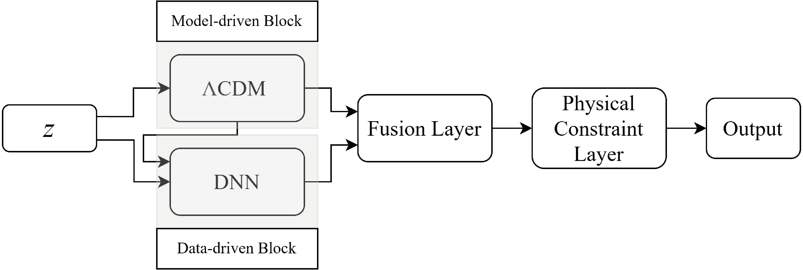

Figure 1.  The architecture of the ResNet consists of two blocks: model-driven and data-driven blocks.

where $ {\boldsymbol{W}}_i $ and $ {\boldsymbol{b}}_i $ denote the weight matrix and bias vector of the ith layer, with dimensions $ m\times n $ and $ m\times 1 $, respectively. Here, m and n correspond to the number of neurons in the current and preceding layers. The number of neurons in the four layers is set to 128, 64, 32, and 1, respectively. For the first layer, the superscripts on the weight matrices distinguish the contributions from the two different inputs. The activation function $ \sigma $ used throughout the network is the rectified linear unit (ReLU), defined as

An exception is made in the third hidden layer during the reconstruction of the target E(z), where we adopt a modified activation function $ \sigma(x) + 1 $ to improve training performance.

The outputs of the model-driven and data-driven blocks are combined in a fusion layer:

where the blending coefficient $ \alpha \in [0,1] $ is a trainable parameter that determines the relative contribution of the model-based and data-driven components. This adaptive weighting mechanism allows the network to dynamically balance theoretical priors with observational information during training.

The Physical Constraint Layer imposes boundary conditions on $ {\boldsymbol{y}}_{\rm{unif}} $ based on physically motivated initial values derived from theoretical considerations. Specifically, we enforce:

The final output layer returns $ {\boldsymbol{y}}_{\rm{pred}} $, the reconstructed target function.

The ResNet is trained by minimizing a loss function defined as the mean squared error (MSE) between the predicted output $ {\boldsymbol{y}}_{\rm{pred}} $ and the corresponding observational data. Unlike previous treatments of observational uncertainties [30−32], we adopt a variance-weighted loss function, ensuring that data points with smaller errors exert proportionally greater influence during training. The optimization is carried out using the Adam optimizer, which adaptively adjusts the learning rate to efficiently locate the minimum of the loss function.

To estimate predictive uncertainties, we adopt the dropout technique as a Bayesian approximation. During training, dropout layers with a fixed dropout rate of 0.5 are applied after the first, second, and third layers of the data-driven block. At inference time, dropout remains active (i.e., Monte Carlo dropout), allowing the network to generate an ensemble of outputs for a given input. This method effectively approximates Bayesian inference without requiring a full probabilistic model and has been shown to yield reliable uncertainty estimates in deep learning frameworks [30, 32, 40].

Deep learning, a rapidly advancing subfield of machine learning, leverages multilayer artificial neural networks to extract complex, non-linear structures from high-dimensional data. In recent years, such techniques have found growing application in cosmology, where they offer a flexible and non-parametric means of reconstructing physical observables from noisy and incomplete datasets [21, 31−33]. Compared with traditional regression or interpolation methods, deep neural networks (DNNs) have proven particularly effective in modeling cosmological functions when the underlying forms are unknown or data coverage is sparse [21, 33]. Here, we adopt a deep learning approach to reconstruct the normalized Hubble parameter E(z) and the comoving distance D(z) based on H(z) and SNe Ia datasets. The derivative of the comoving distance, D'(z), is obtained by numerical differentiation, which requires the reconstructed D(z) curve to be sufficiently smooth. Combining E(z) and D'(z), the curvature diagnostic $ {\cal{O}}_k(z) $ can be model-independently evaluated.

We design a deep neural network architecture based on the residual network (ResNet) framework [41], comprising multiple residual blocks that may incorporate either explicit mathematical functions or neural modules. Our approach incorporates theoretical guidance from $ \Lambda $CDM directly into the learning process, not as a fixed prior but as an auxiliary signal that helps stabilize and guide training. Although the $ \Lambda $CDM model faces both theoretical and observational challenges, it continues to serve as the prevailing framework in modern cosmology and provides a useful reference for assessing the performance of reconstruction methods [21, 30, 32, 33]. It should be noted that, once embedded in the network, the $ \Lambda $CDM form no longer carries cosmological meaning: it acts solely as a mathematical template, with parameters treated as trainable hyperparameters optimized alongside other network hyperparameters, entirely detached from their physical interpretation. This design enables the network to generalize more effectively in under-constrained regions while preserving model independence.

The ResNet architecture was designed to mitigate the degradation problem in deep neural networks, where increased depth leads to diminished performance—not due to overfitting, but owing to optimization difficulties [41]. ResNet addresses this by introducing residual blocks that learn a residual function relative to the input $ {\boldsymbol{x}} $, rather than attempting to learn the desired mapping $ {\boldsymbol{H}}({\boldsymbol{x}}) $ directly. Specifically, each block is structured to compute

where $ {\boldsymbol{F}}({\boldsymbol{x}}) $ denotes the residual function.

This formulation creates two effective computational paths: a residual path that learns the correction $ {\boldsymbol{F}}({\boldsymbol{x}}) $ and an identity path that simply forwards the input. When the optimal representation is already captured at a certain depth, the network can suppress the residual and default to identity mapping, avoiding unnecessary transformation. This property allows additional layers to be added without degrading performance, as they can act as transparent identity mappings if further learning is not needed. Importantly, directly training layers to replicate an identity function is known to be difficult. The residual formulation alleviates this by shifting the learning objective to modeling residuals, which are typically easier to optimize. This innovation enables the successful training of very deep networks and constitutes a key advantage of ResNet over traditional architectures.

The architecture of our ResNet is illustrated in Figure 1 and consists of two distinct components: a model-driven block and a data-driven block. The model-driven component encodes the $ \Lambda $CDM prediction using a single free parameter—the matter density $ \Omega_m $—to generate theoretical outputs $ {\boldsymbol{y}}_{\rm{model}}({\boldsymbol{z}}) $. This block operates directly on redshift inputs and is trained jointly with the rest of the network. The data-driven block is a four-layer fully connected DNN, which receives both the redshift and model prediction as inputs. It is mathematically described by:

Figure 1.  The architecture of the ResNet consists of two blocks: model-driven and data-driven blocks.

where $ {\boldsymbol{W}}_i $ and $ {\boldsymbol{b}}_i $ denote the weight matrix and bias vector of the ith layer, with dimensions $ m\times n $ and $ m\times 1 $, respectively. Here, m and n correspond to the number of neurons in the current and preceding layers. The number of neurons in the four layers is set to 128, 64, 32, and 1, respectively. For the first layer, the superscripts on the weight matrices distinguish the contributions from the two different inputs. The activation function $ \sigma $ used throughout the network is the rectified linear unit (ReLU), defined as

An exception is made in the third hidden layer during the reconstruction of the target E(z), where we adopt a modified activation function $ \sigma(x) + 1 $ to improve training performance.

The outputs of the model-driven and data-driven blocks are combined in a fusion layer:

where the blending coefficient $ \alpha \in [0,1] $ is a trainable parameter that determines the relative contribution of the model-based and data-driven components. This adaptive weighting mechanism allows the network to dynamically balance theoretical priors with observational information during training.

The Physical Constraint Layer imposes boundary conditions on $ {\boldsymbol{y}}_{\rm{unif}} $ based on physically motivated initial values derived from theoretical considerations. Specifically, we enforce:

The final output layer returns $ {\boldsymbol{y}}_{\rm{pred}} $, the reconstructed target function.

The ResNet is trained by minimizing a loss function defined as the mean squared error (MSE) between the predicted output $ {\boldsymbol{y}}_{\rm{pred}} $ and the corresponding observational data. Unlike previous treatments of observational uncertainties [31−33], we adopt a variance-weighted loss function, ensuring that data points with smaller errors exert proportionally greater influence during training. The optimization is carried out using the Adam optimizer, which adaptively adjusts the learning rate to efficiently locate the minimum of the loss function.

To estimate predictive uncertainties, we adopt the dropout technique as a Bayesian approximation. During training, dropout layers with a fixed dropout rate of 0.5 are applied after the first, second, and third layers of the data-driven block. At inference time, dropout remains active (i.e., Monte Carlo dropout), allowing the network to generate an ensemble of outputs for a given input. This method effectively approximates Bayesian inference without requiring a full probabilistic model and has been shown to yield reliable uncertainty estimates in deep learning frameworks [31, 33, 42].

We apply the ResNet-based deep learning framework—implemented in TensorFlow ¹—to reconstruct the dimensionless Hubble parameter E(z) and the comoving distance D(z) from observational datasets, and further obtain the derivative D'(z) through numerical differentiation. Unlike conventional deep learning methods that may yield non-smooth outputs due to their discrete predictions, our ResNet architecture enables smooth function reconstruction, which is essential for reliable numerical differentiation and curvature diagnostics.

Figure 2 shows the reconstruction of E(z) using H(z) measurements. The green line denotes the ResNet output, with 1$ \sigma $ and 2$ \sigma $ credible regions shaded in dark and light blue, respectively. The H(z) data points are shown in red, while the black curve is the reference curve representing the standard $ \Lambda $CDM model with fiducial parameters $ \{\Omega_m,H_0\} = \{0.3,\ 70\ \mathrm{km\ s^{-1}\ Mpc^{-1}} \} $. The reconstruction aligns well with the $ \Lambda $CDM model up to redshift $ z\sim1 $, but exhibits a mild downward deviation at higher redshifts. This deviation is informed by the limited coverage and larger dispersion of the high-z data, suggesting that the network remains sensitive to the observed data and does not simply revert to model expectations in data-sparse regimes.

Figure 2.  (color online) Reconstruction of E(z) from H(z) data using the deep learning method.

The reconstruction of D(z) based on the SN Ia datasets and the corresponding derivatives D'(z) are presented in Figure 3. In all cases, the ResNet produces smooth distance curves with stable numerical derivatives. While the overall trends are mutually consistent, their alignment with $ \Lambda $CDM differs in statistical significance. The reconstructed D(z) from Pantheon+ is consistent with the $ \Lambda $CDM model at the 1$ \sigma $ confidence level across the entire redshift range. By contrast, the reconstructions from Union3 and DESY5 exhibit comparable deviations beyond $ z\sim1.5 $, remaining consistent with the $ \Lambda $CDM model at the 2$ \sigma $ level. These differences likely arise from variations in redshift coverage, sample size, and calibration procedures. Relative to Pantheon+, Union3 exhibits greater dispersion, particularly at $ z>1 $, whereas DESY5 lacks high-redshift leverage beyond $ z\sim1.3 $.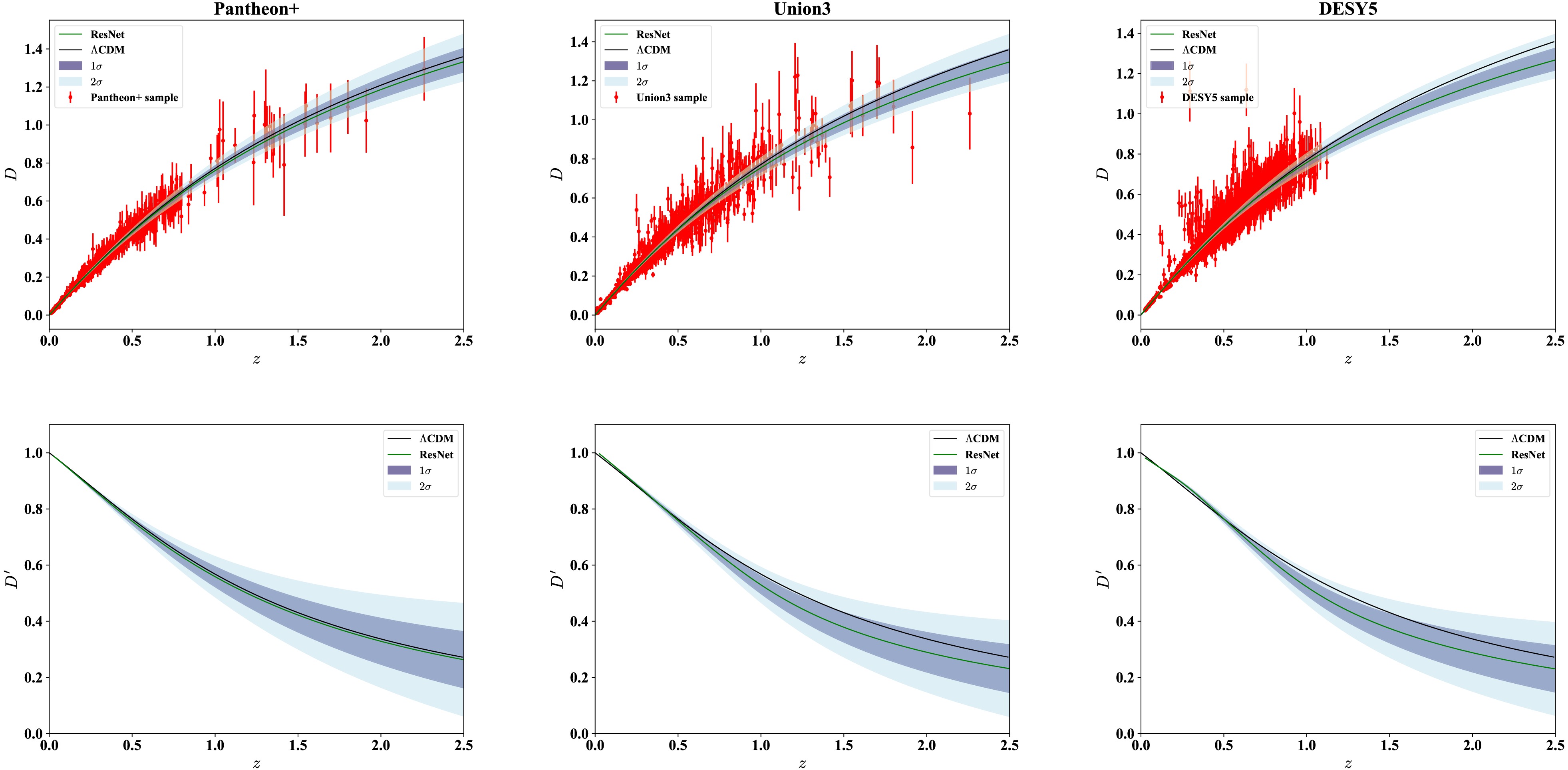

Figure 3.  (color online) Reconstruction of D(z) from three SNe Ia samples, along with the corresponding derivatives D'(z).

The derivative reconstructions further highlight these dataset-dependent distinctions. The D'(z) related to Pantheon+ shows the tightest agreement with the $ \Lambda $CDM curve across the explored range. In contrast, the derivatives related to Union3 and DESY5 display amplified fluctuations, especially in the intermediate- to high-redshift regimes, where their deviations extend to the 2$ \sigma $ level. Although none of these departures reach statistical significance, these differences indicate the sensitivity of derivatives to dataset-specific systematics and the importance of calibration quality in shaping cosmological inferences.

Using the reconstructed E(z) and D'(z), we evaluate the curvature diagnostic function $ {\cal{O}}_k(z) $, defined in Eq. (8), to perform a null test of spatial flatness. Figure 4 presents the resulting diagnostic. The green lines show the central estimate, with 1$ \sigma $ and 2$ \sigma $ uncertainty bands overlaid. The dashed lines correspond to a universe with $ \Omega_k^{(0)}=0 $ and $ \Omega_k^{(0)}=-0.2 $. Across most of the redshift range $ 0<z<2.5 $, $ {\cal{O}}_k(z) $ obtained within Pantheon+ remains consistent with zero within 1$ \sigma $, indicating a spatially flat Universe. However, a systematic downward drift becomes evident at high redshift, indicating a mild preference for negative curvature. Notably, the reconstructed mean value of $ {\cal{O}}_k(z) $ approaches the $ \Omega_k^{(0)}=-0.2 $ line within 1$ \sigma $ over the redshift interval $ 0<z<2.5 $, while it deviates significantly from the flat scenario at high redshift. This behavior primarily originates from the underestimated values of E(z) at high redshift, which propagate into the curvature diagnostic.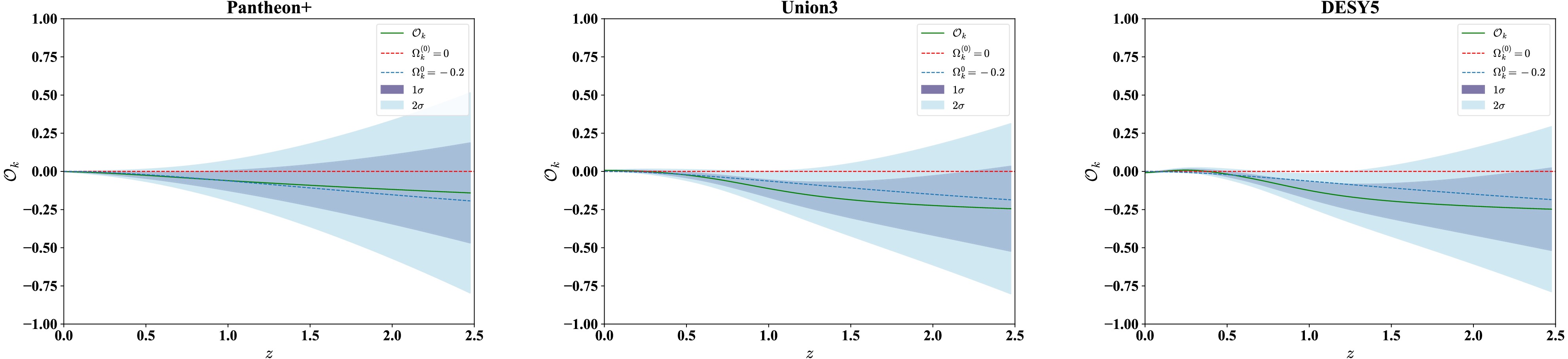

Figure 4.  (color online) Reconstructions of $ {\cal{O}}_k(z) $ from three SNe Ia samples. The dashed lines correspond to a universe with $ \Omega_k^{(0)}=0 $ and $ \Omega_k^{(0)}=-0.2 $, respectively.

The reconstruction based on Union3 is consistent with flatness at low redshift but exhibits a systematic downward drift beyond $ z\sim0.5 $. In this regime, the median curve remains persistently below zero, with the 1$ \sigma $ band no longer fully encompassing the flat line, and approaches the negative-curvature reference. At certain redshifts, the deviation extends toward the 2$ \sigma $ level, suggesting a stronger preference for negative curvature that may reflect sample distribution and intrinsic dispersion within Union3.

The DESY5 reconstruction follows a broadly similar pattern, with the median $ {\cal{O}}_k(z) $ drifting negative at intermediate to high redshifts and approaching the same reference. A distinguishing feature is a small convex upward excursion at $ 0<z<0.5 $, mirrored in the behavior of the derivative D'(z), indicating that this anomaly originates in the DESY5 distance reconstruction itself. Beyond this low-redshift feature, the deviations at higher redshift are comparable in amplitude and significance to those found with Union3.

Taken together, our results indicate that while spatial flatness remains broadly consistent with current datasets, there is a mild and coherent tendency toward negative curvature at high redshift. Although not statistically conclusive, this trend may hint at systematic effects in the high-z Hubble rate measurements or signal potential physics beyond the $ \Lambda $CDM model. In either case, extending the quantity and quality of high-z observations will be crucial for refining curvature constraints and testing the global geometry of spacetime.

We apply the ResNet-based deep learning framework—implemented in TensorFlow ¹—to reconstruct the dimensionless Hubble parameter E(z) and the comoving distance D(z) from observational datasets, and further obtain the derivative D'(z) through numerical differentiation. Unlike conventional deep learning methods that may yield non-smooth outputs due to their discrete predictions, our ResNet architecture enables smooth function reconstruction, which is essential for reliable numerical differentiation and curvature diagnostics.

Figure 2 shows the reconstruction of E(z) using H(z) measurements. The green line denotes the ResNet output, with 1$ \sigma $ and 2$ \sigma $ credible regions shaded in dark and light blue, respectively. The H(z) data points are shown in red, while the black curve is the reference curve representing the standard $ \Lambda $CDM model with fiducial parameters $ \{\Omega_{\rm m},H_0\} = \{0.3,\ 70\ \mathrm{km\ s^{-1}\ Mpc^{-1}} \} $. The reconstruction aligns well with the $ \Lambda $CDM model up to redshift $ z\sim1 $, but exhibits a mild downward deviation at higher redshifts. This deviation is informed by the limited coverage and larger dispersion of the high-z data, suggesting that the network remains sensitive to the observed data and does not simply revert to model expectations in data-sparse regimes.

Figure 2.  (color online) Reconstruction of E(z) from H(z) data using the deep learning method.

The reconstruction of D(z) based on the SN Ia datasets and the corresponding derivatives D'(z) are presented in Fig. 3. In all cases, the ResNet produces smooth distance curves with stable numerical derivatives. While the overall trends are mutually consistent, their alignment with $ \Lambda $CDM differs in statistical significance. The reconstructed D(z) from Pantheon+ is consistent with the $ \Lambda $CDM model at the 1$ \sigma $ confidence level across the entire redshift range. By contrast, the reconstructions from Union3 and DESY5 exhibit comparable deviations beyond $ z\sim1.5 $, remaining consistent with the $ \Lambda $CDM model at the 2$ \sigma $ level. These differences likely arise from variations in redshift coverage, sample size, and calibration procedures. Relative to Pantheon+, Union3 exhibits greater dispersion, particularly at $ z>1 $, whereas DESY5 lacks high-redshift leverage beyond $ z\sim1.3 $.

Figure 3.  (color online) Reconstruction of D(z) from three SNe Ia samples, along with the corresponding derivatives D'(z).

The derivative reconstructions further highlight these dataset-dependent distinctions. The D'(z) related to Pantheon+ shows the tightest agreement with the $ \Lambda $CDM curve across the explored range. In contrast, the derivatives related to Union3 and DESY5 display amplified fluctuations, especially in the intermediate- to high-redshift regimes, where their deviations extend to the 2$ \sigma $ level. Although none of these departures reach statistical significance, these differences indicate the sensitivity of derivatives to dataset-specific systematics and the importance of calibration quality in shaping cosmological inferences.

Using the reconstructed E(z) and D'(z), we evaluate the curvature diagnostic function $ {\cal{O}}_k(z) $, defined in Eq. (8), to perform a null test of spatial flatness. Figure 4 presents the resulting diagnostic. The green lines show the central estimate, with 1$ \sigma $ and 2$ \sigma $ uncertainty bands overlaid. The dashed lines correspond to a universe with $ \Omega_k^{(0)}=0 $ and $ \Omega_k^{(0)}=-0.2 $. Across most of the redshift range $ 0<z<2.5 $, $ {\cal{O}}_k(z) $ obtained within Pantheon+ remains consistent with zero within 1$ \sigma $, indicating a spatially flat Universe. However, a systematic downward drift becomes evident at high redshift, indicating a mild preference for negative curvature. Notably, the reconstructed mean value of $ {\cal{O}}_k(z) $ approaches the $ \Omega_k^{(0)}=-0.2 $ line within 1$ \sigma $ over the redshift interval $ 0<z<2.5 $, while it deviates significantly from the flat scenario at high redshift. This behavior primarily originates from the underestimated values of E(z) at high redshift, which propagate into the curvature diagnostic.

Figure 4.  (color online) Reconstructions of $ {\cal{O}}_k(z) $ from three SNe Ia samples. The dashed lines correspond to a universe with $ \Omega_k^{(0)}=0 $ and $ \Omega_k^{(0)}=-0.2 $, respectively.

The reconstruction based on Union3 is consistent with flatness at low redshift but exhibits a systematic downward drift beyond $ z\sim0.5 $. In this regime, the median curve remains persistently below zero, with the 1$ \sigma $ band no longer fully encompassing the flat line, and approaches the negative-curvature reference. At certain redshifts, the deviation extends toward the 2$ \sigma $ level, suggesting a stronger preference for negative curvature that may reflect sample distribution and intrinsic dispersion within Union3.

The DESY5 reconstruction follows a broadly similar pattern, with the median $ {\cal{O}}_k(z) $ drifting negative at intermediate to high redshifts and approaching the same reference. A distinguishing feature is a small convex upward excursion at $ 0<z<0.5 $, mirrored in the behavior of the derivative D'(z), indicating that this anomaly originates in the DESY5 distance reconstruction itself. Beyond this low-redshift feature, the deviations at higher redshift are comparable in amplitude and significance to those found with Union3.

Taken together, our results indicate that while spatial flatness remains broadly consistent with current datasets, there is a mild and coherent tendency toward negative curvature at high redshift. Although not statistically conclusive, this trend may hint at systematic effects in the high-z Hubble rate measurements or signal potential physics beyond the $ \Lambda $CDM model. In either case, extending the quantity and quality of high-z observations will be crucial for refining curvature constraints and testing the global geometry of spacetime.

In this study, we performed a model-independent null test of the spatial curvature of the Universe by reconstructing the dimensionless Hubble parameter E(z), the comoving distance D(z), and its derivative D'(z) using a deep residual neural network (ResNet) architecture. Our framework combines data-driven flexibility with model-driven prior by integrating theoretical expectations from the $ \Lambda $CDM cosmology directly into the training architecture. This hybrid approach enables stable, interpretable reconstructions of cosmological observables while preserving the independence of the inference from any specific cosmological model. Leveraging H(z) measurements and the current SNe Ia samples, we constructed the curvature diagnostic function $ {\cal{O}}_k(z) = E(z)D'(z)-1 $, which vanishes identically in a spatially flat universe. This provides a direct, geometry-based test of cosmic curvature that does not rely on specific assumptions about the underlying cosmological model.

The reconstruction of E(z) from H(z) data follows the $ \Lambda $CDM expectation up to $ z\sim1 $, but exhibits a mild suppression at higher redshifts, reflecting the limited availability and relatively large uncertainties of high-z measurements. The reconstructions of D(z) across the three supernova samples remain mutually consistent at low redshift but diverge modestly beyond $ z\sim1 $. Pantheon+ yields the smoothest distance curve, closely tracking $ \Lambda $CDM within 1$ \sigma $ across the full range. By contrast, Union3 and DESY5 exhibit larger dispersion at intermediate to high redshift. These distinctions are amplified in the derivatives: D'(z) from Pantheon+ remains in tight agreement with the reference model, whereas Union3 and DESY5 show pronounced fluctuations, with excursions approaching the 2$ \sigma $ level.

Within the Pantheon+ sample, the reconstructed $ {\cal{O}}_k(z) $ remains consistent with zero within 1$ \sigma $ in the redshift range $ 0<z<2.5 $, supporting the assumption of spatial flatness in this regime. At high redshifts, however, a mild downward trend becomes apparent, suggestive of a preference for negative spatial curvature. Although not statistically significant, this trend is qualitatively consistent with previous GP-based analyses [27, 30]. In contrast, reconstructions based on Union3 and DESY5 display a coherent downward shift at intermediate and high redshifts, with median curves departing from zero and indicating a stronger preference for a closed universe. These findings stand in some tension with previous studies [2−4]. For example, within the $ \Lambda $CDM framework, DESY5 has been reported as consistent with flatness, yielding $ \Omega_k=0.16\pm0.16 $ [2], whereas stronger evidence for an open universe has been obtained when combining with non-CMB datasets [3]. Using DESI BAO data and cubic spline reconstruction, Jiang et al. [4] reported $ \Omega_k=0.135\pm0.087 $ for Pantheon+, $ \Omega_k=0.098\pm0.089 $ for Union3, and $ \Omega_k=0.067\pm0.089 $ for DESY5—all suggestive of mild openness. These discrepancies may in part reflect systematics in non-supernova datasets, while a potential underestimation of E(z) from H(z) measurements could also bias our curvature diagnostic low. Together, these results highlight the critical need for more precise high-redshift measurements to robustly constrain cosmic geometry.

Our findings underscore the value of integrating theoretical guidance into the training of neural networks, without compromising the model-independent character of the reconstruction. This hybrid approach enhances training stability, improves interpretability, and yields more accurate predictions—particularly in redshift regimes where observational data are sparse or uncertain. As forthcoming cosmological surveys dramatically expand the quantity and precision of data, the prospects for model-independent inference of fundamental cosmological parameters will be significantly enhanced. In particular, future optical and radio observations are expected to deliver precise measurements of the Hubble parameter H(z) across the redshift range $ 0<z<3 $, with projected relative uncertainties at the 1%~10% level [43, 44]. These improvements will enable more stringent constraints on spatial curvature, independent of assumptions about the underlying cosmological model. Fully leveraging these data will require coordinated reconstructions from heterogeneous observables spanning overlapping redshift ranges. Our results highlight deep learning as a compelling and versatile alternative to traditional regression techniques in cosmology, offering a robust pathway toward high-fidelity reconstructions of the Universe's geometry in the future.

In this study, we performed a model-independent null test of the spatial curvature of the Universe by reconstructing the dimensionless Hubble parameter E(z), the comoving distance D(z), and its derivative D'(z) using a deep residual neural network (ResNet) architecture. Our framework combines data-driven flexibility with model-driven prior by integrating theoretical expectations from the $ \Lambda $CDM cosmology directly into the training architecture. This hybrid approach enables stable, interpretable reconstructions of cosmological observables while preserving the independence of the inference from any specific cosmological model. Leveraging H(z) measurements and the current SNe Ia samples, we constructed the curvature diagnostic function $ {\cal{O}}_k(z) = E(z)D'(z)-1 $, which vanishes identically in a spatially flat universe. This provides a direct, geometry-based test of cosmic curvature that does not rely on specific assumptions about the underlying cosmological model.

The reconstruction of E(z) from H(z) data follows the $ \Lambda $CDM expectation up to $ z\sim1 $, but exhibits a mild suppression at higher redshifts, reflecting the limited availability and relatively large uncertainties of high-z measurements. The reconstructions of D(z) across the three supernova samples remain mutually consistent at low redshift but diverge modestly beyond $ z\sim1 $. Pantheon+ yields the smoothest distance curve, closely tracking $ \Lambda $CDM within 1$ \sigma $ across the full range. By contrast, Union3 and DESY5 exhibit larger dispersion at intermediate to high redshift. These distinctions are amplified in the derivatives: D'(z) from Pantheon+ remains in tight agreement with the reference model, whereas Union3 and DESY5 show pronounced fluctuations, with excursions approaching the 2$ \sigma $ level.

Within the Pantheon+ sample, the reconstructed $ {\cal{O}}_k(z) $ remains consistent with zero within 1$ \sigma $ in the redshift range $ 0<z<2.5 $, supporting the assumption of spatial flatness in this regime. At high redshifts, however, a mild downward trend becomes apparent, suggestive of a preference for negative spatial curvature. Although not statistically significant, this trend is qualitatively consistent with previous GP-based analyses [26, 29]. In contrast, reconstructions based on Union3 and DESY5 display a coherent downward shift at intermediate and high redshifts, with median curves departing from zero and indicating a stronger preference for a closed universe. These findings stand in some tension with previous studies [2−4]. For example, within the $ \Lambda $CDM framework, DESY5 has been reported as consistent with flatness, yielding $ \Omega_k= 0.16\pm 0.16 $ [2], whereas stronger evidence for an open universe has been obtained when combining with non-CMB datasets [3]. Using DESI BAO data and cubic spline reconstruction, Jiang et al. [4] reported $ \Omega_k=0.135\pm0.087 $ for Pantheon+, $ \Omega_k=0.098\pm0.089 $ for Union3, and $ \Omega_k= 0.067\pm 0.089 $ for DESY5—all suggestive of mild openness. These discrepancies may in part reflect systematics in non-supernova datasets, while a potential underestimation of E(z) from H(z) measurements could also bias our curvature diagnostic low. Together, these results highlight the critical need for more precise high-redshift measurements to robustly constrain cosmic geometry.

Our findings underscore the value of integrating theoretical guidance into the training of neural networks, without compromising the model-independent character of the reconstruction. This hybrid approach enhances training stability, improves interpretability, and yields more accurate predictions—particularly in redshift regimes where observational data are sparse or uncertain. As forthcoming cosmological surveys dramatically expand the quantity and precision of data, the prospects for model-independent inference of fundamental cosmological parameters will be significantly enhanced. In particular, future optical and radio observations are expected to deliver precise measurements of the Hubble parameter H(z) across the redshift range $ 0<z<3 $, with projected relative uncertainties at the 1%~10% level [41–42]. These improvements will enable more stringent constraints on spatial curvature, independent of assumptions about the underlying cosmological model. Fully leveraging these data will require coordinated reconstructions from heterogeneous observables spanning overlapping redshift ranges. Our results highlight deep learning as a compelling and versatile alternative to traditional regression techniques in cosmology, offering a robust pathway toward high-fidelity reconstructions of the Universe's geometry in the future.