Axisymmetric generalization of zero-scalar-curvature solutions from the Schwarzschild metric via Newman-Janis algorithm

The Newman-Janis algorithm (NJA) [1] is a method used to derive axisymmetric black hole spacetimes from spherically symmetric ones. The term "off-shell" refers to the fact that these generated spacetimes do not necessarily satisfy the gravitational field equations [2]. This limitation has led to criticism because axisymmetric black holes obtained via the NJA often fail to meet these equations. For example, although the NJA can generate an axisymmetric black hole in the Chern-Simons gravity, the Pontryagin density is non-zero, indicating a failure to satisfy the field equations [3].

The original NJA was formulated in terms of the Newman-Penrose formalism [4]. It involves applying a complex transformation, followed by a change of coordinates or parameters, to derive a rotating solution [5]. However, a modified version [6] of the NJA has been introduced, which eliminates the need for this additional complex coordinate transformation. Its most notable success came from reproducing Kerr black holes ¹ and discovering Kerr-Newman black holes in the Einstein-Maxwell theory [7, 8]. Given the observational relevance and diverse applications of rotating black holes [9−13], the NJA has become a popular tool for constructing various types of axisymmetric black holes [14−17]. Despite this, the efforts continue [18−20] to understand the algorithm's underlying physical basis. As time goes on, the NJA has evolved into two distinct branches: one that retains the Newman-Penrose formalism [6, 21, 22] and the other that no longer relies on tetrads [5, 23].

In this work, we apply the NJA within the Newman-Penrose formalism but omit the complexification of variables and parameters. Our goal is to derive a general complex transformation for Schwarzschild black holes that yields axisymmetric black holes with zero-scalar-curvature metrics. ² In other words, we aim to explore how many zero-scalar-curvature and axisymmetric black holes can be generated from Schwarzschild black holes by using the NJA. We refer to these solutions as the Newman-Janis (NJ) class of Schwarzschild black holes, emphasizing NJA’s potential as a classification tool for axisymmetric black holes. In general, the black holes derived from the same seed solution should belong to one NJ class because they share the key physical properties [18].

The structure of the paper is as follows. In Sec. 2, we begin by applying a modified version of the NJA [6] to retrieve Taub-NUT black holes from the Schwarzschild seed metric. We emphasize the function freedoms in the process of retrieving Taub-NUT black holes, which motivates a generalization of the modified NJA in Sec. 3, where we also present a formal metric for axisymmetric black holes resulting from general complex transformations. In Sec. 4, we focus on the zero-scalar-curvature condition and derive the explicit form of the complex transformations introduced in the previous section. Sec. 5 explores a new type of axisymmetric black holes predicted by our treatment. The final section, Sec. 6, gives our conclusion, followed by two appendices detailing the specific forms of two curvature invariants.

In this section, we introduce the approach used [6] for Kerr black holes and extend it to Taub-NUT black holes, aiming to further generalize this approach in the subsequent section. The term "non-complexified" refers to the fact that this approach does not require extending coordinates and parameters into the complex domain. We start with the seed metric for a spherically symmetric spacetime,

where $ \mathrm{d}\Omega^2_2 = \mathrm{d} \theta^2 + \sin^2\theta \mathrm{d}\phi^2 $ is the metric of a unit two-sphere.

The first step is to rewrite this metric in the Newman-Penrose tetrad formalism. We introduce the advanced null coordinate,

which transforms the above metric to

This can then be expressed in terms of the Newman-Penrose tetrad as

where $ l^\mu $, $ n^\mu $, and $ m^\mu $ are null vectors, and $ \bar{m}^\mu $ is the complex conjugate of $ m^\mu $. The explicit form of the tetrad vectors is given by

The next step is our proposal: We generalize the functions $ f(r) $, $ g(r) $, and $ h(r) $ to $ F(r, N) $, $ G(r, N) $, and $ H(r, N) $, ensuring that they reduce to their original forms when the NUT charge N vanishes,

This relation serves as a boundary condition for the subsequent calculations. We then introduce a complex coordinate transformation, ³

substitute it into Eq. (5), and give the following tetrad,

Using this tetrad and Eq. (4), we generalize the metric as follows:

The above treatment differs from the traditional one applied to Taub-NUT black holes in Ref. [2] where the mass parameter is also transformed by $ M \to M' = M - \mathrm{i} N $.

To express the above metric in the Boyer–Lindquist coordinates, we perform the following coordinate transformation,

After considering the conditions $ g_{tr} = g_{r\phi} = 0 $, we derive

which are required by the axisymmetric and stationary preconditions. Then, using the boundary condition given by Eq. (6), we obtain

In the case of Schwarzschild black holes, where $ f = g = 1 - 2M/r $, we find

Following the procedure outlined in Ref. [6] for the Kerr case, we choose for the Taub-NUT case,

and solve F from Eq. (11),

We note that the choice of λ, Eq. (14), is based on our experience and familiarity with the Taub-NUT black hole metric. Later, we will show how the equations of motion, $ R^\mu_{\;\;\nu} = 0 $, along with the boundary conditions Eq. (6), can be used to determine the exact forms of the functions $ F(r, N) $, $ G(r, N) $, and $ H(r, N) $.

By setting $ F = G $, we have

The choice of $ F = G $ stems from the characteristics of the seed metric, i.e., $ f = g $ in the Schwarzschild case.

Finally, by fixing $ H = \sqrt{r^2 + N^2} $, we recover the Taub-NUT black hole metric [24],

where $ \Sigma = r^2 + N^2 $. The choice of H, similar to that of λ, will be discussed in further detail. Before proceeding, we offer some remarks on the overall process.

In Eq. (11), the equation $ \chi = 0 $ reduces the number of free functions compared to the case of Kerr black holes [6], but it leaves H undetermined, requiring it to be manually fixed. In Table 1 we compare the function freedoms between Taub-NUT and Kerr black holes in the framework of the NJA.

	f	g	h	F	G	H	λ	$ {\chi} $
Taub-NUT BHs	giv	giv	giv	det	det	semi	semi	det
Kerr BHs	giv	giv	giv	det	det	det	semi	semi

Table 1.  The function freedoms.

In Table 1, the "giv" denotes "given", meaning the function is initially provided as a condition. The "det" refers to "determined", indicating that the function can be formally calculated if other functions are known. The "semi" denotes "semi-determined", meaning that the asymptotic behavior of the function with respect to a certain parameter is known, but its explicit form is inferred from the target metric. The table shows that, for the NJ class of Schwarzschild black holes, there are only two free functions that need to be fixed based on experience or unknown conditions. When χ is fixed to be zero, the remaining function H becomes free for Taub-NUT black holes. On the other hand, χ becomes free for Kerr black holes when H is fixed.

The presence of two semi-determined functions in the NJA suggests introducing additional conditions to fully determine them. The equations of motion provide a natural choice for this purpose. According to it, the NJA can partially circumvent the traditional challenge of being considered to be an off-shell method. We begin with the metric in the Boyer–Lindquist coordinates,

where we have used $ F = G $ and replaced λ and χ by

in Eq. (9) under the coordinate transformation Eq. (10). Our goal is to use the vacuum equations of motion, $ R^\mu_{\;\nu} = 0 $, along with the boundary conditions from Eq. (6), to give the explicit forms of F and H. In Sec. 4, when we address the general case, we will extend the vacuum equations discussed here to encompass the zero-scalar-curvature condition.

We begin by noting $ R^2_{\;2} = R^3_{\;3} $, which reduces the equations of motion to the following three independent equations,

From Eq. (20a), we derive the solution for F,

where $ c_1 $ and $ c_2 $ are constants of integration.

Substituting this expression for F into Eq. (20b), we arrive at the equation,

which leads to the solution for H,

where $ c_3 $ and $ c_4 $ are also integration constants. By substituting this result for H back into the expression Eq. (21) for F, we obtain

Finally, substituting these results into the third equation, Eq. (20c), allows us to determine the integration constants through the following relation,

Thus, Eqs. (23), (24), and (25) provide the general solutions to the equations of motion, Eq. (20).

We now proceed to determine the constants of integration using the conditions provided in Eq. (6). At first, applying the condition,

we find

Next, we derive $ c_2 $ from Eq. (25),

where we have omitted the periodicity inherent in the trigonometric function. Substituting $ c_2 $, $ c_3 $, and $ c_4 $ into Eq. (24), we obtain

Next, applying the boundary condition,

we deduce that the parameter $ c_1 $ must be $ 4M^2 $ plus a N-dependent function that vanishes as $ N\to 0 $. Considering the balance of dimensions, we arrive at

Therefore, we have retrieved the metric of Taub-NUT black holes without arbitrarily assigning specific forms to any function at any stage of the above derivation.

Our new treatment demonstrates that, starting from the Schwarzschild metric and applying the complex transformation in Eq. (7), the Taub-NUT metric is the unique solution that satisfies the vacuum equations of motion $ R_{\mu\nu}=0 $.

In this section, we derive the forms of λ and χ using a kind of matching conditions ⁴ instead of specifying the initial transformations. Our goal is to generalize the NJA for Schwarzschild black holes by introducing a broader class of transformations.

To extend our treatment from the previous section to arbitrary transformations, we consider a generalized complex transformation of Eq. (7),

where the functions $ \alpha(\theta, p) $ and $ \beta(\theta, p) $ depend on certain parameters that are denoted collectively by p, such as the NUT charge in Eq. (7). For simplicity, we use p to represent any relevant parameter and just use the symbols $ \alpha(\theta) $ and $ \beta(\theta) $ but know in our mind that α and β depend on p.

At first, we extend the functions in the seed metric, originally appeared in the advanced null coordinate in Eq. (3), and derive the following null tetrad by substituting Eq. (32) into Eq. (5),

where the prime stands for the derivative with respect to θ and the functions $ F(r, \theta, p) $, $ G(r, \theta, p) $, and $ H(r, \theta, p) $ depend on the parameter p and satisfy the matching condition,

This condition must be met because, for a given transformation Eq. (32), the axisymmetric black holes produced by the NJA related to the functions G, F, and H reduce to the original spherically symmetric metric Eq. (1) related to f, g, and h, as the parameter p approaches zero. Following the procedure for deriving Eq. (9) but replacing Eqs. (7) and (8) by Eqs. (32) and (33), respectively, we give the following metric,

Secondly, when the transformation Eq. (10) is applied with the replacement of N by p, the conditions $ g_{tr} = g_{r\phi} = 0 $ lead to the following solutions ⁵ for $ \lambda(r, p) $ and $ \chi(r, p) $:

Following the reasoning stated in the previous section, see the contexts from Eqs. (10)-(12) and the relevant analysis in Ref. [6], we propose the following forms of $ \lambda(r) $ and $ \chi(r) $ as $ {p \to 0} $,

where b, c, and d are free parameters. Before continuing calculations, the following two points deserve attentions:

● Only one of $ \alpha'(\theta) $ and $ \beta'(\theta) $ can be zero. If both are zero, no modification occurs to the seed metric or to the null tetrad. If $ \alpha'(\theta) $ is zero and $ F = G $, both F and H can be determined; but if $ \beta'(\theta) $ is zero, only F can be determined, leaving H undetermined. This indicates that it may not fix all free functions to use the equations of motion alone. Therefore, we will first examine the case of $ \beta'(\theta) \neq 0 $.

● The assumption in Eq. (37) is motivated by the form of Eq. (36) and the matching condition in Eq. (34), which is quite general. However, for a specific case, such as the case of Taub-NUT black holes, the formulation Eq. (14) is inferred directly from the Taub-NUT metric in Eq. (17).

Lastly, when $ f = g $ in the seed metric, it is reasonable to assume $ F(r, \theta) = G(r, \theta) $. From Eqs. (36) and (37), we can express $ F(r, \theta) $ as

and determine the function $ H(r, \theta) $ due to $ \beta'(\theta) \neq 0 $,

For the Schwarzschild metric where $ f = g = 1 - 2M/r $ and $ h = r $, the resulting metric components of Eq. (35) take the forms,

If the metric described by the above components satisfies the condition of a vanishing Ricci curvature, it belongs to the NJ class of Schwarzschild black holes, which will be discussed in the next section.

The spacetime produced by the NJA is asymptotically flat as long as $ \beta' $ does not vanish. As $ r \to \infty $, the Ricci curvature scalar behaves as

Furthermore, the formulation of Ricci scalar R and Kretschmann scalar $ K\equiv R^{\mu}_{\nu\alpha\beta}R_{\mu}^{\nu\alpha\beta} $ contains the denominator $ 8 [\beta'(\theta )]^3 \left[c \alpha '(\theta )\sin\theta +d+r^2\right]^3 $, thus there is a potential curvature singularity at $ r_s $ given by

If $ r_s $ is not real for all values of θ, the metric describes a regular black hole spacetime. The event horizon is determined by the singularity of $ g_{11} $,

which is analogous to the horizon of Kerr black holes.

In this section, we aim to explore whether it can yield additional zero-scalar-curvature black hole solutions by applying the NJA to Schwarzschild black holes. Specifically, we seek the general forms of the functions $ \alpha(\theta) $ and $ \beta(\theta) $ that satisfy the condition $ R = 0 $, indicating the zero scalar-curvature. ⁶ We note that the zero scalar-curvature is a less stringent condition than the vacuum Einstein equations, $ R^\mu_{\;\nu} = 0 $. Although any metric that satisfies the vacuum Einstein equations must be zero-scalar-curvature, a zero-scalar-curvature metric may not satisfy the Einstein equations. A zero-scalar-curvature metric can correspond to the scenarios involving a traceless energy-momentum tensor, $ \text{Tr} T^{\mu}_{\;\;\nu}=0 $. An additional issue arises concerning the interpretation of the NJA. Traditionally, the NJA has been understood primarily as a method for introducing rotation into a static black hole solution. However, it can also alter other physical properties, such as generating a nonzero NUT charge. The observation that the energy-momentum tensor has zero trace may evoke similarities with electrodynamics and prompt the question of whether the NJA could similarly introduce electric charge into an initially uncharged BH. From the perspective of symmetry, if the seed solution possesses an axisymmetric distribution of electric or magnetic charge, our construction method does not exclude the possibility of such charges emerging in our new solution. Therefore, our idea is applicable to searching for new axisymmetric black holes from a spherically symmetric seed black hole in gravity coupled to other fields.

To proceed, we express the Ricci scalar R as a polynomial in r,

where $ R_{n,i} $, $ i = 0, \dots, 4 $, are the coefficients given in App. A, the subscript n is the abbreviation of $ numerator $, and the denominator takes the form,

Similar to the subscript n in the numerator of R, the subscript d means $ denominator $.

To solve $ R = 0 $, we require $ R_{n,i} = 0 $, resulting in five equations. Solving $ R_{n,1} = 0 $ yields two possible forms for $ \beta(\theta) $,

where $ c_1 $ and $ c_2 $ are constants of integration. The first solution, $ \beta(\theta) = c_1 $, leads to both the numerator and denominator of the Ricci scalar vanishing, making the ratio indeterminate, so we discard it. Thus, we only keep the second solution Eq. (47).

The equation $ R_{n,4} = 0 $ yields a nonlinear differential equation,

Additionally, the equations $ R_{n,0} = 0 $ and $ R_{n,2} = 0 $ lead to the same equation as Eq. (48) if $ \alpha' $ is replaced by the solution in Eq. (47). As a result, there are only two independent equations, ⁷ $ R_{n,1}=0 $ and $ R_{n,4}=0 $, among the five ones, $ R_{n,i} = 0 $, $ i = 0, \dots, 4 $. To solve Eq. (48), we first note the presence of trigonometric terms and the absence of the function $ \beta(\theta) $ itself. Such a property suggests a substitution to simplify the equation. We define the new variables,

with which we transform the original nonlinear differential equation Eq. (48) into

To further simplify, we employ the ansatz:

which changes the equation into

Its solution is given by

where $ c_3 $ and $ c_4 $ are constants of integration. This solution provides a general form for $ \beta'(x) $, which can now be integrated to obtain the desired transformation functions.

Now we are able to derive $ \beta(\theta) $ from $ y = \beta' $,

where $ c_5 $ is constant of integration. Next, we determine $ \alpha(\theta) $ by using the second expression in Eq. (46),

where $ c_6 $ is constant of integration. By substituting α and β back into Eq. (40), we derive the general NJ class of Schwarzschild black holes. Notably, both α and β do not depend on the parameter b because the equations $ R_{n,1}=0 $ and $ R_{n,4}=0 $ do not involve b.

We now examine the parameters $ (b, c, d) $ and constants $ (c_2, c_3, c_4, c_5, c_6) $ in the solutions given by Eqs. (54) and (55). At first, although $ \alpha' $ and $ \beta' $ rather than α and β appear in the tetrad and metric, we cannot set $ c_5 = c_6 = 0 $. As we will demonstrate later, the non-zero values of $ c_5 $ and $ c_6 $ are essential for obtaining the correct Taub-NUT black hole. Secondly, we note that Eq. (40c) presents potential singularities at $ \theta = 0 $ and π due to the presence of $ \csc \theta $. It is crucial to choose the constants in α and β to eliminate any divergence in the metric at these two angles. Since $ \alpha' $ depends solely on θ, $ \beta' $ will play a key role in addressing these singularities in $ g_{22} $. Expanding $ g_{22} $ around $ \theta = 0 $ up to the constant order, we find

To avoid the divergence at $ \theta = 0 $, the constant $ c_3 $ must satisfy the conditions $ c_3 \ge 1 $ or $ c_3 \le -1 $. A similar analysis shows that these conditions also apply to avoid the divergence at $ \theta = \pi $.

Next, the parameters $ (b, c, d) $ and constants $ (c_2, c_3, c_4, c_5, c_6) $ are further constrained by the fundamental energy conditions [25, 26]. These conditions ensure that the physical interpretation of the spacetime remains consistent with the energy distribution:

● Weak Energy Condition (WEC): The components of Einstein’s tensor satisfy $ -G^0_{\;0} \geq 0 $ and $ -G^0_{\;0} + G^i_{\;i} > 0 $. This condition asserts that the total energy density, as measured by any observer following a timelike trajectory, is always non-negative.

● Dominant Energy Condition (DEC): This condition requires $ -G^0_{\;0} \geq 0 $ and $ -G^0_{\;0} \geq |G^i_{\;i}| $, ensuring that the energy flux remains causal and that the energy-momentum propagates at or below the speed of light.

● Strong Energy Condition (SEC): Here, $ -G^0_{\;0} + \sum_i G^i_{\;i} \geq 0 $ and $ -G^0_{\;0} + G^i_{\;i} > 0 $. This implies that the gravitational interaction tends to attract, as demonstrated by the convergence of timelike and null geodesic congruences, even when negative mass-energy densities are present.

The energy conditions impose nonlinear inequalities on the parameters and constants. Solving these inequalities analytically is generally infeasible. Instead, they are possiblely suited for being verified whether a constructed axisymmetric black hole meets the required energy conditions.

Let us now consider a specific example by assigning particular values to the parameters and constants. Choosing,

where a denotes the angular momentum parameter of rotating black holes, we obtain the forms of $ \alpha(\theta) $ and $ \beta(\theta) $ corresponding to Kerr black holes,

Alternatively, by choosing

we can derive the functions $ \alpha(\theta) $ and $ \beta(\theta) $ for Kerr-Taub-NUT black holes from Eqs. (54) and (55),

which reduce to those of pure Taub-NUT black holes when setting $ a = 0 $.

Our proposal differs from the treatment of Ref. [20], where the authors generalized the seed metric from Schwarzschild black holes to any spherically symmetric black hole and then adopted the NJA. Our focus is on complex transformations; specifically, we have identified Schwarzschild black holes as the seed and correspondingly propose the general NJ transformations, where these transformations ensure that the resulting metric satisfies the zero-scalar-curvature condition.

In this section, we provide a new example of zero-scalar-curvature black holes derived from the Schwarzschild type using the NJA. The metric is constructed by selecting the following parameters and constants,

where $ \mathfrak{a} $ is a parameter which is used to replace c and $ b\pi $. Using these values in Eqs. (54) and (55), we obtain $ \alpha(\theta) $ and $ \beta(\theta) $ as follows,

which can be seen as a deformation of Eq. (58) corresponding to Kerr black holes. Further, substituting Eq. (62) into the general solutions given by Eq. (40), we derive the metric components of a new zero-scalar-curvature black hole,

Since the general expressions Eqs. (54) and (55) are obtained by solving the condition $ R=0 $, any specific parameter choice, such as in Eq. (61), necessarily ensures that the equation of motion $ R=0 $ is satisfied. In particular, the resulting metric in Eq. (63) must also satisfy $ R=0 $, which can be explicitly verified by substituting Eq. (63) into the Ricci scalar.

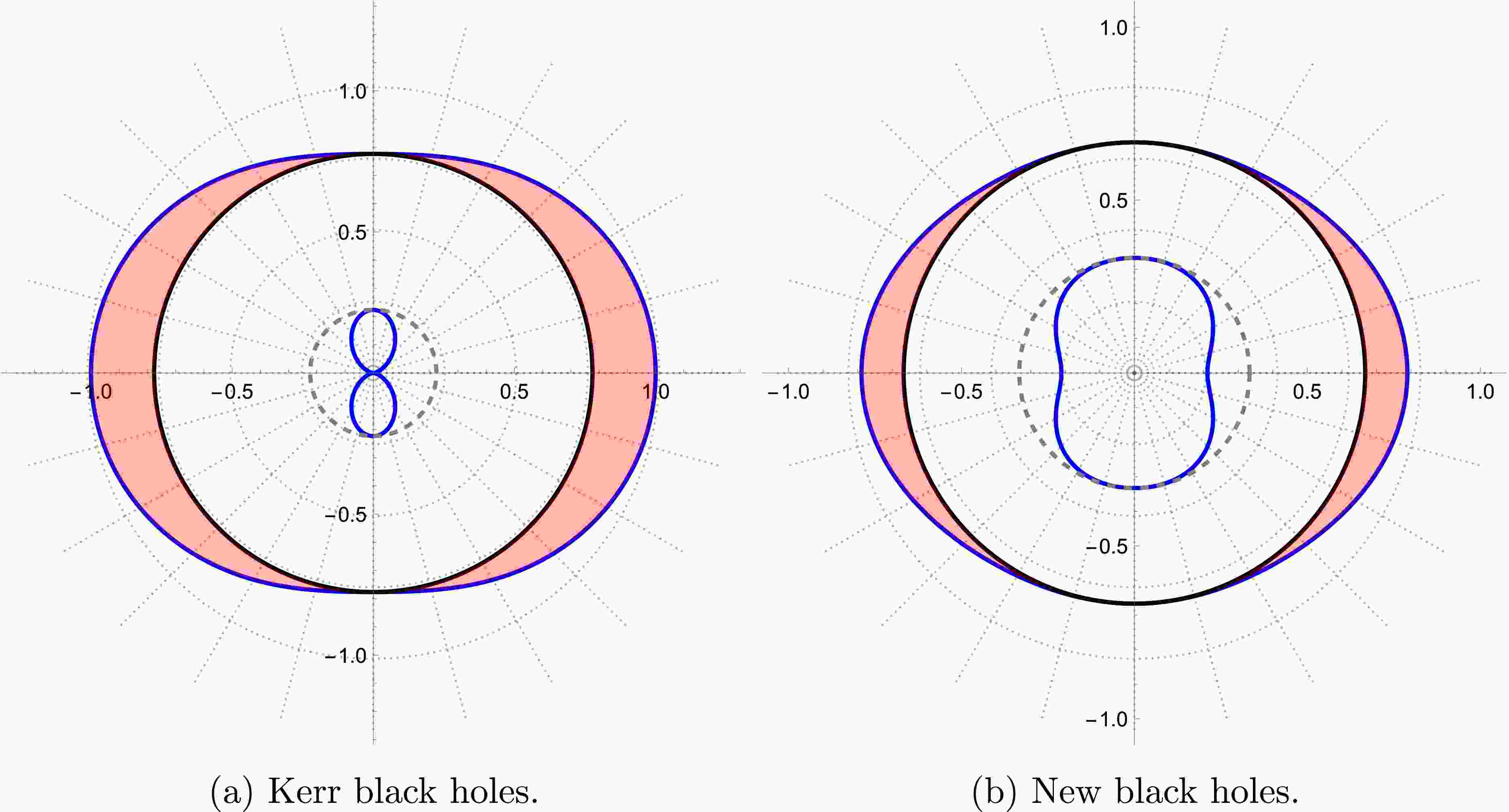
The horizons are determined by the solutions of $ 1/g_{11} = 0 $, yielding $ r_\pm = M \pm \sqrt{M^2 - \pi^2 \mathfrak{a}^2} $. The infinite redshift surfaces, characterized by the radius $ r_{rs} $, are depicted by the condition $ g_{00} = 0 $,

We compare the structure of infinite redshift surfaces, depicted by Eq. (64), with that of Kerr black holes in the polar slice using the Boyer–Lindquist coordinates, as shown in Fig. 1. In this figure, the blue curves indicate the outer and inner radii of the infinite redshift surfaces, while the solid black and dashed gray curves represent the outer and inner horizons, respectively. The pink shadows denote the black hole ergospheres. Notably, the infinite redshift surfaces exhibit comparable deformations, particularly at $ \theta = 0 $.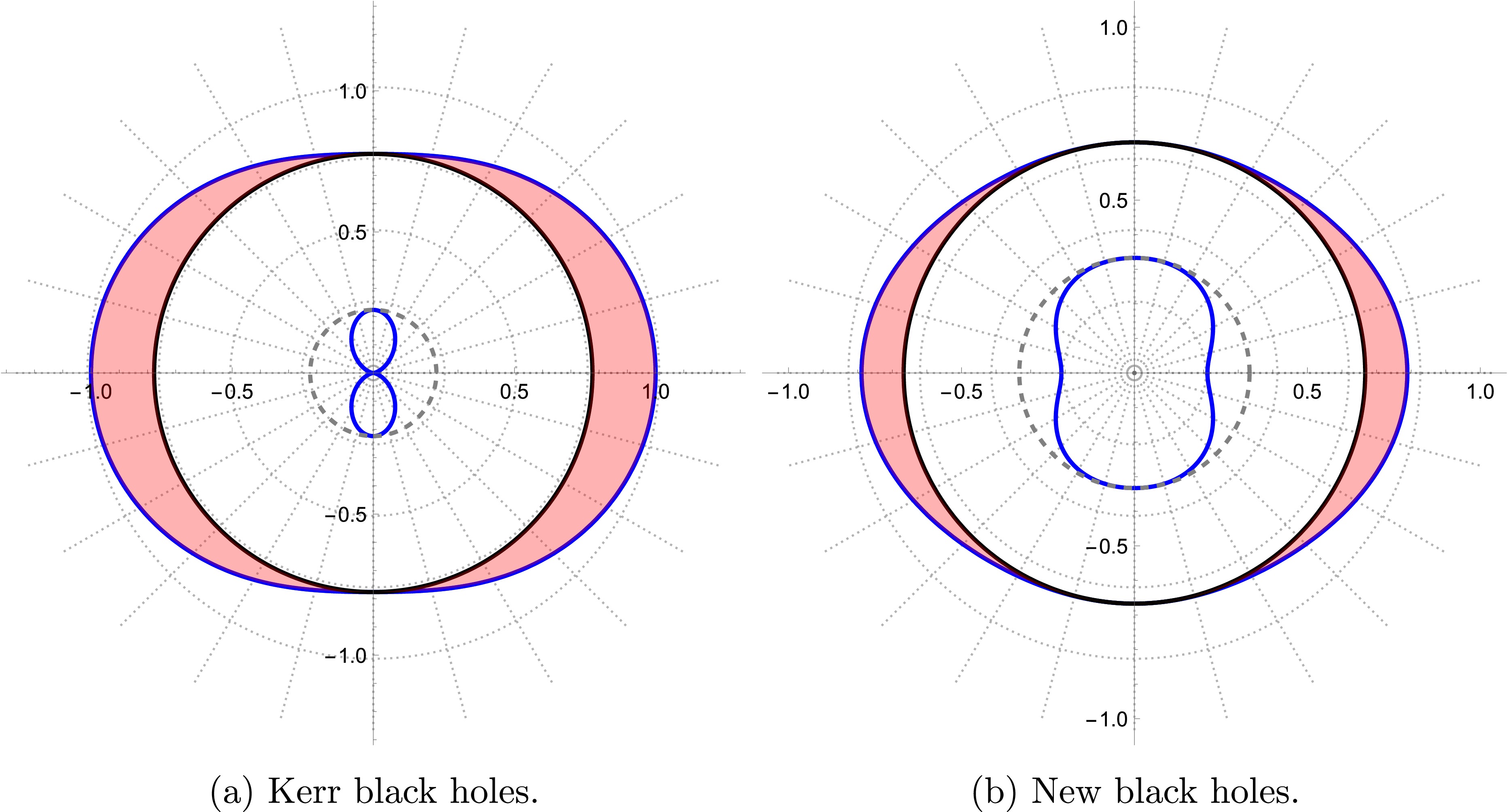

Figure 1.  (color online) Polar slices in the Boyer–Lindquist coordinates.

To assess the existence of singularities in the spacetime, we compute the Kretschmann scalar,

where the coefficients $ K_{n,i} $ are provided in App. (B), and the denominator is given by

The real roots of $ K_d $ occur at $ r = 0 $ and $ \cos\theta = 0 $, similar to the roots found in Kerr black holes, indicating that these black holes possess a singular loop rather than a singular point. Moreover, the Kretschmann scalar of our solution differs from that of the known Kerr and Taub–NUT spacetimes. This allows us to conclude that the resulting black hole cannot be obtained from either Kerr or Taub–NUT through a coordinate transformation since the Kretschmann scalar is independent of the choice of coordinates.

Finally, we conclude this section with an analysis of the mechanical and thermodynamic properties of the new black hole. To compute the relevant quantities and compare them with those of the Kerr solution, it is essential to emphasize that our discussion is carried out within Einstein’s theory of gravity. This point is important because not all thermodynamic information is determined solely by the spacetime metric; for instance, the entropy also depends on the underlying gravitational action. Next, we compare the new black hole with the Kerr black hole in the properties of Hawking temperature, Berkenstein-Hawking entropy, and angular velocity if the two black holes have the same mass and the parameter $ \mathfrak{a} $ is equivalent to the angular momentum per mass of Kerr black holes $ a^{\rm{Kerr}} $.

Since the new axisymmetric black hole described by Eq. (63) is solved within Einstein’s theory of gravity, it is expected to obey the relation that the Hawking temperature is proportional to the surface gravity. That is, it is suitable to compare the surface gravity of the two black holes. The surface gravity of the new black hole can be computed from the following relation,

where Ω is the angular velocity given by Eq. (72). Thus, we obtain

For the Kerr black hole, its surface gravity is [27, 28]

It is obvious that $ \kappa\neq \kappa_{\rm{Kerr}} $ even if the two black holes have the same mass and $ \mathfrak{a}=a^{\rm{Kerr}} $ ⁸.

We turn to the Bekenstein–Hawking entropy. According to the Bekenstein–Hawking area law, the entropy is proportional to [29] the horizon area, $ S = A/4 $. We can compute the horizon area from Eq. (63),

by integrating the surface with $ t=\text{const.} $ and $ r=r_+ $. For comparison, the horizon area of Kerr black holes takes the form,

which is obviously different from Eq. (70).

The angular velocity at the event horizon can be obtained [27, 28] from the tangent null vector $ l^\alpha=(1,0,0,\Omega) $, yielding

which represents the angular velocity of light rays relative to an observer at infinity, and can be interpreted as the black hole’s angular velocity. For comparison, the angular velocity of a Kerr black hole has the form,

which is also different from Eq. (72).

In this work, we aim to construct the axisymmetric black holes that satisfy the zero-scalar-curvature condition and can be generated by the NJA from Schwarzschild black holes as the seed metric. We successfully derive the general forms of complex transformations and the corresponding axisymmetric metrics. Our results include Kerr, Taub-NUT, and Kerr-Taub-NUT black holes as special cases for different choices of parameters. Additionally, our findings indicate the existence of new axisymmetric black holes, which we designate as the NJ class of Schwarzschild black holes.

The methodology developed in this study may be extended to related areas. For instance, it could be applied to construct axisymmetric black holes in the Chern-Simons gravity. This would involve inverting the specific form of complex transformations when the vanishing Pontryagin density is imposed as a constraint. Another possible application is the construction of regular black holes [30] that satisfy the relevant equations of motion. Notably, there exists a class of regular black holes that does not originate from quantum corrections, such as the ABG black holes [31], the solutions to the gravity coupled to nonlinear electrodynamics, where the corresponding equations of motion should be imposed for searching axisymmetric black holes besides the zero-scalar-curvature condition. Moreover, for the regular black holes derived from quantum corrections [32−35], our method may also facilitate the generation of axisymmetric solutions that meet specific conditions. This will be the focus of our future research.

Here we display the coefficients of the numerator in Eq. (44).

Here we display the coefficients of the numerator in Eq. (65).