


 Abstract
 HTML
HTML Reference
 Related
 PDF
PDF


HTML
-
In a previous paper [1], we studied the lepton number violation decays of the
${B}_{c}^{-}$ meson induced by a doubly-charged Higgs boson. There are both experimental and theoretical motivations to study this kind of particle. Although the Higgs boson has been found, whether it is the one predicted by the Standard Model still needs more confirmation. It is possible that an extended Higgs sector exists, and that there are additional isospin multiplet scalar fields. For example, the SU(2)L triplet scalar, which contains a doubly-charged component, is introduced to generate small neutrino mass in the Type-Ⅱ seesaw modes [2-5]. Generally, such a triplet representation is needed in the left-right symmetric models [6-8] to break the extended SU(2)L × SU(2)R × U(1)B−L symmetry in the Standard Model. The doubly-charged scalar also appears in other models, such as little Higgs models [9] and Georgi-Machacek model [10]. As it can decay into two leptons with the same charge, indicating lepton number violation, such processes for top quark, τ− [11], and charged mesons, such as K−, D−,${D}_{s}^{-}$ , B− [12-15] have been investigated extensively. As the lower bound of the mass of the doubly-doubly charged Higgs boson is around 800 GeV [16, 17], these low energy processes have extremely small branching ratios. Although it is not likely that these channels will be detected soon, as experiments collect more data, the upper limits of the branching ratios for such decay processes will become more stringent. One can also use them to derive further constraints for the effective short-range interactions [18].In Ref. [1], we considered both the three-body and four-body decay channels of
${B}_{c}^{-}$ meson, in which the lepton number is not conserved. In this paper, we investigate the lepton number violation processes of the neutral flavored mesons induced by the doubly-charged Higgs boson. Contrary to the charged meson case, where the annihilation-type diagram and the two W meson emitting diagram both contribute to the amplitude, in the case of the neutral meson, the light antiquark is just a spectator (see Fig. 1). Theoretically, this makes the calculation simpler, as there is no complexity brought by the cascade decay. As for the decay products, the two leptons have the same charge, and so do the two mesons. These decay modes have no equivalent in the Standard Model, which makes them also interesting experimentally.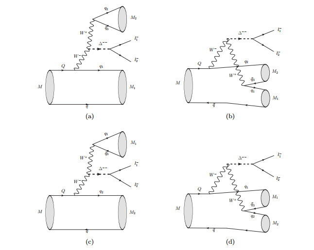
Figure 1. Feynman diagrams of the decay processes
$h\to {h}_{1}{h}_{2}{l}_{1}^{-}{l}_{2}^{-}$ .These channels can also be induced by Majorana-type neutrinos. Their Feynman diagrams are similar to Fig. 1, but the s channels should be replaced by t channels. If the neutrino mass were around GeV, it could be produced on-shell, which has attracted much attention [19-22]. For the cases when the neutrino mass is very small or very large, the branching ratios will have the same order of magnitude as in the case of the doubly-charged Higgs boson [15, 23]. Therefore, the theoretical analysis of the low energy processes induced by the doubly-charged Higgs boson also provides a useful complement to the Majorana neutrino scenario.
This paper is organized as follows. In Sec. 2, we give the Lagrangian which describes the couplings between the Higgs triplet and the Standard Model particles, and present the amplitudes and phase space integrals. In Sec. 3, we give the branching ratios of all decay channels and compare the results for D0 with experimental data. We summarize our results in the last section. Some details of the meson wave functions are presented in the Appendix.
-
The hypothetical Higgs triplet Δ in the 2 × 2 representation is defined as [12]
$ \begin{eqnarray}\Delta =\left(\begin{array}{cc}{\Delta }^{+}/\sqrt{2}&{\Delta }^{++}\\ {\Delta }^{0}&-{\Delta }^{+}/\sqrt{2}\end{array}\right).\end{eqnarray} $
(1) It mixes with the usual SU(2)L Higgs doublet by a mixing angle θΔ, from which we define sΔ = sinθΔ and cΔ = cosθΔ.
The Lagrangian which describes the interaction between Δ and W− gauge boson or SM fermions has the following form [12, 15]
$ \begin{eqnarray}\begin{array}{ll}{ {\mathcal L} }_{{\rm{int}}}^{\prime}=&{\rm{i}}{h}_{ij}{\psi }_{iL}^{T}C{\sigma }_{2}\Delta {\psi }_{jL}-\sqrt{2}g{m}_{W}{s}_{\Delta }{\Delta }^{++}{W}^{-\mu }{W}_{\mu }^{-}\\ &+\displaystyle \frac{\sqrt{2}}{2}g{c}_{\Delta }{W}^{-\mu }{\Delta }^{-}{\overleftrightarrow{\partial }}_{\mu }{\Delta }^{++}\\ &+\displaystyle \frac{{\rm{i}}g{s}_{\Delta }}{\sqrt{2}{m}_{W}{c}_{\Delta }}{\Delta }^{+}({m}_{{q}^{\prime}}{\bar{q}}_{R}{q}_{R}^{\prime}-{m}_{q}{\bar{q}}_{L}{q}_{L}^{\prime})+{\rm{H}}.{\rm{c}}., \end{array}\end{eqnarray} $
(2) where C = iγ2γ0 is the charge conjugation matrix; ψiL represents the leptonic doublet; hij is the leptonic Yukawa coupling constant; g is the weak coupling constant. The third and fourth terms represent the interactions between the singly-charged boson and the other particles. Compared with the second term, their contributions can be neglected.
If q = q3, all four diagrams in Fig. 1 contribute to the decay:
$ \begin{eqnarray}\begin{array}{ll}{ {\mathcal M} }_{A}&=\displaystyle \frac{{g}^{3}}{8\sqrt{2}{m}_{W}^{3}}{V}_{{q}_{1}Q}{V}_{{q}_{2}{q}_{3}}\displaystyle \frac{{s}_{\Delta }{h}_{ij}}{{m}_{\Delta }^{2}}\langle {h}_{1}({p}_{1}){h}_{2}({p}_{2})|{({\bar{q}}_{1}Q)}_{V-A}{({\bar{q}}_{2}{q}_{3})}_{V-A}|h(p)\rangle \langle {\rm{lepton}}\rangle \\ &=\displaystyle \frac{{g}^{3}}{8\sqrt{2}{m}_{W}^{3}}{V}_{{q}_{1}Q}{V}_{{q}_{2}{q}_{3}}\displaystyle \frac{{s}_{\Delta }{h}_{ij}}{{m}_{\Delta }^{2}}{f}_{{h}_{2}}{p}_{2}^{\mu }\langle {h}_{1}({p}_{1})|{\bar{q}}_{1}{\gamma }_{\mu }(1-{\gamma }_{5})Q|h(p)\rangle \langle {\rm{lepton}}\rangle, \end{array}\end{eqnarray} $
(3) $ \begin{eqnarray}\begin{array}{ll}{ {\mathcal M} }_{B}&=\displaystyle \frac{{g}^{3}}{8\sqrt{2}{m}_{W}^{3}}{V}_{{q}_{2}Q}{V}_{{q}_{1}{q}_{3}}\displaystyle \frac{{s}_{\Delta }{h}_{ij}}{{m}_{\Delta }^{2}}\langle {h}_{1}({p}_{1}){h}_{2}({p}_{2})|{({\bar{q}}_{2}Q)}_{V-A}{({\bar{q}}_{1}{q}_{3})}_{V-A}|h(p)\rangle \langle {\rm{lepton}}\rangle \\ &=\displaystyle \frac{{g}^{3}}{8\sqrt{2}{m}_{W}^{3}}\displaystyle \frac{1}{3}{V}_{{q}_{2}Q}{V}_{{q}_{1}{q}_{3}}\displaystyle \frac{{s}_{\Delta }{h}_{ij}}{{m}_{\Delta }^{2}}{f}_{{h}_{2}}{p}_{2}^{\mu }\langle {h}_{1}({p}_{1})|{\bar{q}}_{1}{\gamma }_{\mu }(1-{\gamma }_{5})Q|h(p)\rangle \langle {\rm{lepton}}\rangle, \end{array}\end{eqnarray} $
(4) $ \begin{eqnarray}\begin{array}{ll}{ {\mathcal M} }_{C}&=\displaystyle \frac{{g}^{3}}{8\sqrt{2}{m}_{W}^{3}}{V}_{{q}_{2}Q}{V}_{{q}_{1}{q}_{3}}\displaystyle \frac{{s}_{\Delta }{h}_{ij}}{{m}_{\Delta }^{2}}\langle {h}_{1}({p}_{1}){h}_{2}({p}_{2})|{({\bar{q}}_{2}Q)}_{V-A}{({\bar{q}}_{1}{q}_{3})}_{V-A}|h(p)\rangle \langle {\rm{lepton}}\rangle \\ &=\displaystyle \frac{{g}^{3}}{8\sqrt{2}{m}_{W}^{3}}{V}_{{q}_{2}Q}{V}_{{q}_{1}{q}_{3}}\displaystyle \frac{{s}_{\Delta }{h}_{ij}}{{m}_{\Delta }^{2}}{f}_{{h}_{1}}{p}_{1}^{\mu }\langle {h}_{2}({p}_{2})|{\bar{q}}_{2}{\gamma }_{\mu }(1-{\gamma }_{5})Q|h(p)\rangle \langle {\rm{lepton}}\rangle, \end{array}\end{eqnarray} $
(5) $ \begin{eqnarray}\begin{array}{ll}{ {\mathcal M} }_{D}&=\displaystyle \frac{{g}^{3}}{8\sqrt{2}{m}_{W}^{3}}{V}_{{q}_{1}Q}{V}_{{q}_{2}{q}_{3}}\displaystyle \frac{{s}_{\Delta }{h}_{ij}}{{m}_{\Delta }^{2}}\langle {h}_{1}({p}_{1}){h}_{2}({p}_{2})|{({\bar{q}}_{1}{q}_{3})}_{V-A}{({\bar{q}}_{2}Q)}_{V-A}|h(p)\rangle \langle {\rm{lepton}}\rangle \\ &=\displaystyle \frac{{g}^{3}}{8\sqrt{2}{m}_{W}^{3}}\displaystyle \frac{1}{3}{V}_{{q}_{1}Q}{V}_{{q}_{2}{q}_{3}}\displaystyle \frac{{s}_{\Delta }{h}_{ij}}{{m}_{\Delta }^{2}}{f}_{{h}_{1}}{p}_{1}^{\mu }\langle {h}_{2}({p}_{2})|{\bar{q}}_{2}{\gamma }_{\mu }(1-{\gamma }_{5})Q|h(p)\rangle \langle {\rm{lepton}}\rangle, \end{array}\end{eqnarray} $
(6) where the factor
$\displaystyle \frac{1}{3}$ in${ {\mathcal M} }_{B}$ and${ {\mathcal M} }_{D}$ is introduced by the Fierz transformation; ⟨lepton⟩ is the leptonic part of the transition matrix element; Vqiqj is the Cabibbo-Kobayashi-Maskawa matrix element. The definition of the decay constant fh1 of a pseudoscalar meson$ \begin{eqnarray}\langle {h}_{1}({p}_{1})|{\bar{q}}_{1}{\gamma }^{\mu }(1-{\gamma }_{5}){q}_{2}|0\rangle ={\rm{i}}{f}_{{h}_{1}}{p}_{1}^{\mu }\end{eqnarray} $
(7) is used. For vector mesons, it should be replaced by
$ \begin{eqnarray}\langle {h}_{1}({p}_{1}, \epsilon )|{\bar{q}}_{1}{\gamma }^{\mu }(1-{\gamma }_{5}){q}_{2}|0\rangle ={M}_{1}{f}_{{h}_{1}}{\epsilon }^{\mu }.\end{eqnarray} $
(8) The values of the decay constants are given in Table 1. It should be pointed out that we have used the factorization assumption in Eqs. (3)-(6), which is not quite appropriate when both final mesons are light. However, as only the order of magnitude is important in such processes, we anticipate that the effects of nonfactorization and final meson interactions do not change the results significantly.
fπ fK fK* fρ fD fDs fD* $ {f}_{{D}_{s}^{\ast }} $ 130.4 156.2 217 205 204.6 257.5 340 375 Finally, we get the transition amplitude
$ \begin{eqnarray}\begin{array}{ll} {\mathcal M} &={ {\mathcal M} }_{A}+{ {\mathcal M} }_{B}+{ {\mathcal M} }_{C}+{ {\mathcal M} }_{D}\\ &=\displaystyle \frac{{g}^{3}{s}_{\Delta }{h}_{ij}}{8\sqrt{2}{m}_{W}^{3}{m}_{\Delta }^{2}}\{({V}_{{q}_{1}Q}{V}_{{q}_{2}{q}_{3}}+\displaystyle \frac{1}{3}{V}_{{q}_{2}Q}{V}_{{q}_{1}{q}_{3}}){f}_{{h}_{2}}{p}_{2}^{\mu }\\ &\times \langle {h}_{1}({p}_{1})|{\bar{q}}_{1}{\gamma }_{\mu }(1-{\gamma }_{5})Q|h(p)\rangle \\ &+({V}_{{q}_{2}Q}{V}_{{q}_{1}{q}_{3}}+\displaystyle \frac{1}{3}{V}_{{q}_{1}Q}{V}_{{q}_{2}{q}_{3}}){f}_{{h}_{1}}{p}_{1}^{\mu }\\ &\times \langle {h}_{2}({p}_{2})|{\bar{q}}_{2}{\gamma }_{\mu }(1-{\gamma }_{5})Q|h(p)\rangle \}\langle {\rm{lepton}}\rangle .\end{array}\end{eqnarray} $
(9) If q ≠ q3, only Fig. 1(a) and (b) contribute:
$ \begin{eqnarray}\begin{array}{ll} {\mathcal M} &={ {\mathcal M} }_{A}+{ {\mathcal M} }_{B}\\ &=\displaystyle \frac{{g}^{3}{s}_{\Delta }{h}_{ij}}{8\sqrt{2}{m}_{W}^{3}{m}_{\Delta }^{2}}({V}_{{q}_{1}Q}{V}_{{q}_{2}{q}_{3}}+\displaystyle \frac{1}{3}{V}_{{q}_{2}Q}{V}_{{q}_{1}{q}_{3}}){f}_{{h}_{2}}{p}_{2}^{\mu }\\ &\times \langle {h}_{1}({p}_{1})|{\bar{q}}_{1}{\gamma }_{\mu }(1-{\gamma }_{5})Q|h(p)\rangle \langle {\rm{lepton}}\rangle .\end{array}\end{eqnarray} $
(10) The hadronic transition matrix can be expressed as [27]
$ \begin{eqnarray}\langle {h}_{1}({p}_{1})|{V}^{\mu }|h(p)\rangle ={f}_{+}({Q}^{2}){(p+{p}_{1})}^{\mu }+{f}_{-}({Q}^{2}){(p-{p}_{1})}^{\mu }, \end{eqnarray} $
(11) where h1 is a pseudoscalar meson, and f+ and f− are form factors. If h1 is a vector meson, we have
$ \begin{eqnarray}\begin{array}{ll}\langle {h}_{1}({p}_{1}, \epsilon )|{V}^{\mu }|h(p)\rangle =&-{\rm{i}}\displaystyle \frac{2}{M+{M}_{1}}{f}_{V}({Q}^{2}){\epsilon }^{\mu {\epsilon }^{\ast }p{p}_{1}}, \\ \langle {h}_{1}({p}_{1}, \epsilon )|{A}^{\mu }|h(p)\rangle =&{f}_{1}({Q}^{2})\displaystyle \frac{{\epsilon }^{\ast }\cdot p}{M+{M}_{1}}{(p+{p}_{1})}^{\mu }\\ &+{f}_{2}({Q}^{2})\displaystyle \frac{{\epsilon }^{\ast }\cdot p}{M+{M}_{1}}{(p-{p}_{1})}^{\mu }\\ &+{f}_{0}({Q}^{2})(M+{M}_{1}){\epsilon }^{\ast \mu }, \end{array}\end{eqnarray} $
(12) where fV and fi (i = 0, 1, 2) are form factors; M and M1 are the masses of corresponding mesons; the definition Q = p − p1 is used.
By applying the Bethe-Salpeter method with the instantaneous approximation [28], the hadronic matrix element is written as
$ \begin{eqnarray}\begin{array}{l} \langle {h}_{1}({p}_{1})|{\bar{q}}_{1}{\gamma }^{\mu }(1-{\gamma }_{5})Q|h(p)\rangle \\ =\displaystyle \int \displaystyle \frac{{{\rm{d}}}^{3}q}{{(2\pi )}^{3}}{\rm{Tr}}\left[\displaystyle \frac{\rlap{/}{p}}{M}\overline{{\varphi }_{{p}_{1}}^{++}}({\overrightarrow{q}}_{1}){\gamma }_{\mu }(1-{\gamma }_{5}){\varphi }_{p}^{++}(\overrightarrow{q})\right], \end{array}\end{eqnarray} $
(13) where φ++ is the positive energy part of the wave function;
$\overrightarrow{q}$ and${\overrightarrow{q}}_{1}$ are the relative three-momenta between the quarks and antiquarks in the initial and final mesons, respectively.The partial decay width is obtained by evaluating the phase space integral
$ \begin{eqnarray}\begin{array}{ll}\Gamma =&\left(1-\displaystyle \frac{1}{2}{\delta }_{{h}_{1}{h}_{2}}\right)\left(1-\displaystyle \frac{1}{2}{\delta }_{{l}_{1}{l}_{2}}\right)\displaystyle \int \displaystyle \frac{{\rm{d}}{s}_{12}}{{s}_{12}}\displaystyle \int \displaystyle \frac{{\rm{d}}{s}_{34}}{{s}_{34}}\\ &\times \displaystyle \int {\rm{d}}\cos {\theta }_{12}\displaystyle \int {\rm{d}}\cos {\theta }_{34}\displaystyle \int {\rm{d}}\phi {\mathcal{K}}| {\mathcal M} {|}^{2}, \end{array}\end{eqnarray} $
(14) where
$ \begin{eqnarray}\begin{array}{ll}{\mathcal{K}}=&\displaystyle \frac{1}{{2}^{15}{\pi }^{6}{M}^{3}}{\lambda }^{1/2}({M}^{2}, {s}_{12}, {s}_{34}){\lambda }^{1/2}({s}_{12}, {M}_{1}^{2}, {M}_{2}^{2})\\ &\times {\lambda }^{1/2}({s}_{34}, {m}_{1}^{2}, {m}_{2}^{2}).\end{array}\end{eqnarray} $
(15) We also use the definitions s12 = (p1 + p2)2 and s34 = (p3 + p4)2. The meanings of θ12, θ34, and ϕ are shown in Fig. 2. δl1l2 is 1 if l1 and l2 are identical particles, otherwise it is 0. The same is true for δh1h2. The integral limits are
$ \begin{eqnarray}\begin{array}{l} {s}_{12}\in [{({M}_{1}+{M}_{2})}^{2}, \ {(M-{m}_{1}-{m}_{2})}^{2}], \\ {s}_{34}\in [{({m}_{1}+{m}_{2})}^{2}, \ {(M-\sqrt{{s}_{12}})}^{2}], \\ \phi \in [0, \ 2\pi ], \ \ \ {\theta }_{12}\in [0, \ \pi ], \ \ \ {\theta }_{34}\in [0, \ \pi ], \end{array}\end{eqnarray} $
(16) 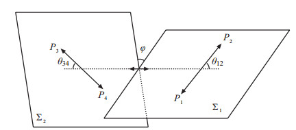
Figure 2. Kinematics of the four-body decay of h in its rest frame. P1 and P2 are respectively the momenta of h1 and h2 in their center-of-momentum frame; P3 and P4 are respectively the momenta of l1 and l2 in their center-of-momentum frame.
where M2, m1, and m2 are the masses of h2, l1, and l2, respectively.
-
The Bethe-Salpeter method has certain advantages when calculating the form factors, especially in the case when both initial and final mesons are heavy. In the first step, the wave functions of the mesons, which include relativistic corrections, are obtained by solving numerically the corresponding instantaneous Bethe-Salpeter equation. Their pole structure is important for describing the properties of heavy mesons. Subsequently, the form factors for the physically allowed region are calculated using Eq. (13) without any analytic extension. Although the instantaneous approximation is reasonable for the double heavy mesons and acceptable for the heavy-light mesons, it results in large errors for the light mesons, such as π and K. For example, when we change the parameters by ±5%, the form factors at Q2 = 0 for the channels with heavy mesons change by less than 10%, while for those with π or K, the errors can be larger than 50%. For processes with light mesons, such as B → π(ρ), other methods are more appropriate, for example the light-cone sum rules. Nevertheless, we use this approximation also for the light mesons as the decay channels we consider are related to new physics, for which the branching ratios are expected to be very small, and only the order of magnitude is important.
The parameters of the doubly-charged Higgs boson have no definite values at present, only the lower or upper limits from experiments are available. For example, the latest results of the ATLAS and CMS Collaborations [16, 17] show that the mass of Δ++ is larger than 800 GeV. From Ref. [12], the upper limit for sΔ is 0.0056. The constraints for the coupling hee can be extracted from the e+e− annihilation process [29]:
$\displaystyle \frac{{h}_{ee}^{2}}{{m}_{\Delta }^{2}}\le 9.7\times {10}^{-6}\ {{\rm{GeV}}}^{-2}$ . For hμμ, the Muon g − 2 experiment provides the limit [30]:$\displaystyle \frac{{h}_{\mu \mu }^{2}}{{m}_{\Delta }^{2}}\le 3.4\times {10}^{-6}\ {{\rm{GeV}}}^{-2}$ . The heμ is related to μ− → e−e+e− and μ− → e− γ processes [12], which give$\displaystyle \frac{{h}_{e\mu }{h}_{ee}}{{m}_{\Delta }^{2}}\le 3.2\times {10}^{-11}\ {{\rm{GeV}}}^{-2}$ and$\displaystyle \frac{{h}_{e\mu }{h}_{\mu \mu }}{{m}_{\Delta }^{2}}\le 2.0\times {10}^{-10}\ {{\rm{GeV}}}^{-2}$ , respectively. Taking mΔ = 1000 GeV as an example, we can estimate the upper limits of the quantity${(\displaystyle \frac{{s}_{\Delta }{h}_{ij}}{{m}_{\Delta }^{2}})}^{2}$ for the ee and μμ cases as 3.0 × 10⁻¹⁶ and 1.1 × 10⁻¹⁶, respectively. For the eμ case, following the method applied in Ref. [12], we let hee and hμμ equal to their upper bound, and get heμ ≤ 1.1 × 10⁻¹⁶, which leads to${(\displaystyle \frac{{s}_{\Delta }{h}_{e\mu }}{{m}_{\Delta }^{2}})}^{2}\le 3.3\times {10}^{-27}$ .For
${\bar{K}}^{0}$ , there are only three channels allowed by the phase space, namely${\pi }^{+}{\pi }^{+}{l}_{1}^{-}{l}_{2}^{-}\ ({l}_{i}=e, \ \mu )$ . The corresponding diagrams are Fig. 1(a)-(d). The π+π+e−e− channel has the largest branching ratio, which is of the order of 10−30 (see Table 2). Experimentally,$Br({K}^{+}\to {\pi }^{-}{l}_{1}^{+}{l}_{2}^{+})\lesssim {10}^{-10}$ [31], which is the most precise result for lepton number violation. However, lepton number violation in four-body decay channels of this particle has not been experimentally found. In Refs. [32, 33], the channels KL, S → π+π−e+e− are investigated. We hope that the${K}_{L, S}\to {\pi }^{+}{\pi }^{+}{l}_{1}^{-}{l}_{2}^{-}$ channels will be experimentally studied in the future.decay channel upper limit of Br ${\bar{K}}^{0}\to {\pi }^{+}{\pi }^{+}{e}^{-}{e}^{-}$ 2.2 × 10⁻³⁰ ${\bar{K}}^{0}\to {\pi }^{+}{\pi }^{+}{\mu }^{-}{\mu }^{-}$ 5.8 × 10⁻³³ ${\bar{K}}^{0}\to {\pi }^{+}{\pi }^{+}{e}^{-}{\mu }^{-}$ 1.3 × 10−41 Table 2. The upper limit of Br for different decay channels of
${\bar{K}}^{0}$ .For D0, the final mesons can be pseudoscalars or vectors. The results for the case when h1 and h2 are both pseudoscalars, that is ππ, πK, or KK, are given in Table 3. The largest value is of the order of magnitude of 10−29. We note that the Fermilab E791 Collaboration presented the upper limits of the branching ratios for these channels [34], which are of the order of 10−5. By comparing the theoretical predictions and experimental data, we find the upper limit of the constant
$\displaystyle \frac{{s}_{\Delta }{h}_{ij}}{{m}_{\Delta }^{2}}$ of the order of 104 GeV−2. One can also extract this upper limit from the three-body decay processes, such as D− → π+e−e−, which gives about 102 GeV−2 by using the results in Ref. [12]. The branching ratios of D0 decay channels, where h1 and h2 are 0−1− or 1−1−, are given in Table 4; the largest value has the order of magnitude of 10−29.decay channel upper limit of Br Exp. bound on Br [34] $ \displaystyle \frac{{s}_{\Delta }{h}_{ij}}{{m}_{\Delta }^{2}} $ /GeV−2D0 → π−π−e+e+ 1.8 × 10⁻²⁹ < 11.2 × 10⁻⁵ < 42734 D0 → π−π−μ+μ+ 7.2 × 10⁻³⁰ < 2.9 × 10⁻⁵ < 21080 D0 → π−π−e+μ+ 4.1 × 10−40 < 7.9 × 10⁻⁵ < 25371 D0 → π−K−e+e+ 7.1 × 10⁻²⁹ < 20.6 × 10⁻⁵ < 29548 D0 → π−K−μ+μ+ 2.7 × 10⁻²⁹ < 39.0 × 10⁻⁵ < 39855 D0 → π−K−e+μ+ 1.5 × 10−39 < 21.8 × 10⁻⁵ < 21683 D0 → K−K−e+e+ 6.1 × 10⁻³⁰ < 15.2 × 10⁻⁵ < 86661 D0 → K−K−μ+μ+ 2.3 × 10⁻³⁰ < 9.4 × 10⁻⁵ < 67045 D0 → K−K−e+μ+ 1.3 × 10−40 < 5.7 × 10⁻⁵ < 38177 Table 3. The upper limit of Br for 0−0− decay channels of D0.
decay channel upper limit of Br decay channel upper limit of Br D0 → π−ρ−e+e+ 2.8 × 10⁻³⁰ D0 → ρ−ρ−e+e+ 6.7 × 10⁻³¹ D0 → π−ρ−μ+μ+ 9.9 × 10⁻³¹ D0 → ρ−ρ−μ+μ+ 1.3 × 10⁻³¹ D0 → π−ρ−e+μ+ 5.8 × 10−41 D0 → ρ−ρ−e+μ+ 9.4 × 10−42 D0 → π−K*−e+e+ 4.8 × 10⁻³⁰ D0 → ρ−K*−e+e+ 2.1 × 10⁻³⁰ D0 → π−K*−μ+μ+ 1.6 × 10⁻³⁰ D0 → ρ−K*−e+μ+ 1.2 × 10−41 D0 → π−K*−e+μ+ 9.5 × 10−41 D0 → K−K*−e+e+ 9.4 × 10⁻³² D0 → ρ−K−e+e+ 1.4 × 10⁻²⁹ D0 → K−K*−μ+μ+ 2.2 × 10⁻³² D0 → ρ−K−μ+μ+ 4.2 × 10⁻³⁰ D0 → K−K*−e+μ+ 1.5 × 10−42 D0 → ρ−K−e+μ+ 2.6 × 10−40 D0 → K*−K*−e+e+ 1.2 × 10⁻³² Table 4. The upper limit of Br for 0−1− and 1−1− decay channels of D0.
The results for
${\bar{B}}^{0}$ and${\bar{B}}_{s}^{0}$ are given in Tables 5-10. The largest value is of the order of 10−28. In Ref. [35], the four-body decay channel B− → D0π+μ−μ− was measured to have a branching ratio of less than 1.5 × 10⁻⁶. There are no experimental values available at present for the neutral B meson decay channels. However, as LHCb is continuing to run, more data will be available. We expect that the LHCb Collaboration will detect such decay modes and will set more stringent constraints on the parameters of doubly-charged Higgs boson. Besides, the future B-factories, such as Belle-Ⅱ, will also have the possibility of providing more information about these channels.decay channel upper limit of Br decay channel upper limit of Br ${\bar{B}}^{0}\to {\pi }^{+}{\pi }^{+}{e}^{-}{e}^{-}$ 7.1 × 10⁻³⁰ ${\bar{B}}^{0}\to {\pi }^{+}{D}_{s}^{+}{e}^{-}{\mu }^{-}$ 1.4 × 10−40 ${\bar{B}}^{0}\to {\pi }^{+}{\pi }^{+}{\mu }^{-}{\mu }^{-}$ 2.8 × 10⁻³⁰ ${\bar{B}}^{0}\to {K}^{+}{D}^{+}{e}^{-}{e}^{-}$ 5.2 × 10⁻³⁰ ${\bar{B}}^{0}\to {\pi }^{+}{\pi }^{+}{e}^{-}{\mu }^{-}$ 1.6 × 10−40 ${\bar{B}}^{0}\to {K}^{+}{D}^{+}{\mu }^{-}{\mu }^{-}$ 2.0 × 10⁻³⁰ ${\bar{B}}^{0}\to {\pi }^{+}{K}^{+}{e}^{-}{e}^{-}$ 2.7 × 10⁻³¹ ${\bar{B}}^{0}\to {K}^{+}{D}^{+}{e}^{-}{\mu }^{-}$ 1.2 × 10−40 ${\bar{B}}^{0}\to {\pi }^{+}{K}^{+}{\mu }^{-}{\mu }^{-}$ 1.1 × 10⁻³¹ ${\bar{B}}^{0}\to {D}^{+}{D}^{+}{e}^{-}{e}^{-}$ 5.3 × 10⁻³⁰ ${\bar{B}}^{0}\to {\pi }^{+}{K}^{+}{e}^{-}{\mu }^{-}$ 6.2 × 10−42 ${\bar{B}}^{0}\to {D}^{+}{D}^{+}{\mu }^{-}{\mu }^{-}$ 2.1 × 10⁻³⁰ ${\bar{B}}^{0}\to {\pi }^{+}{D}^{+}{e}^{-}{e}^{-}$ 7.8 × 10⁻²⁹ ${\bar{B}}^{0}\to {D}^{+}{D}^{+}{e}^{-}{\mu }^{-}$ 1.2 × 10−40 ${\bar{B}}^{0}\to {\pi }^{+}{D}^{+}{\mu }^{-}{\mu }^{-}$ 3.0 × 10⁻²⁹ ${\bar{B}}^{0}\to {D}^{+}{D}_{s}^{+}{e}^{-}{e}^{-}$ 7.2 × 10⁻²⁹ ${\bar{B}}^{0}\to {\pi }^{+}{D}^{+}{e}^{-}{\mu }^{-}$ 1.7 × 10−39 ${\bar{B}}^{0}\to {D}^{+}{D}_{s}^{+}{\mu }^{-}{\mu }^{-}$ 2.9 × 10⁻²⁹ ${\bar{B}}^{0}\to {\pi }^{+}{D}_{s}^{+}{e}^{-}{e}^{-}$ 6.2 × 10⁻³⁰ ${\bar{B}}^{0}\to {D}^{+}{D}_{s}^{+}{e}^{-}{\mu }^{-}$ 1.6 × 10−39 ${\bar{B}}^{0}\to {\pi }^{+}{D}_{s}^{+}{\mu }^{-}{\mu }^{-}$ 2.4 × 10⁻³⁰ Table 5. The upper limit of Br for 0−0− decay channels of
${\bar{B}}^{0}$ .decay channel upper limit of Br decay channel upper limit of Br ${\bar{B}}^{0}\to {\pi }^{+}{\rho }^{+}{e}^{-}{e}^{-}$ 6.4 × 10⁻³⁰ ${\bar{B}}^{0}\to {\rho }^{+}{D}_{s}^{+}{e}^{-}{e}^{-}$ 3.8 × 10⁻³¹ ${\bar{B}}^{0}\to {\pi }^{+}{\rho }^{+}{\mu }^{-}{\mu }^{-}$ 2.5 × 10⁻³⁰ ${\bar{B}}^{0}\to {\rho }^{+}{D}_{s}^{+}{\mu }^{-}{\mu }^{-}$ 1.5 × 10⁻³¹ ${\bar{B}}^{0}\to {\pi }^{+}{\rho }^{+}{e}^{-}{\mu }^{-}$ 1.5 × 10−40 ${\bar{B}}^{0}\to {\rho }^{+}{D}_{s}^{+}{e}^{-}{\mu }^{-}$ 8.7 × 10−42 ${\bar{B}}^{0}\to {\pi }^{+}{K}^{\ast +}{e}^{-}{e}^{-}$ 5.1 × 10⁻³¹ ${\bar{B}}^{0}\to {K}^{+}{D}^{\ast +}{e}^{-}{e}^{-}$ 4.0 × 10⁻³⁰ ${\bar{B}}^{0}\to {\pi }^{+}{K}^{\ast +}{\mu }^{-}{\mu }^{-}$ 2.0 × 10⁻³¹ ${\bar{B}}^{0}\to {K}^{+}{D}^{\ast +}{\mu }^{-}{\mu }^{-}$ 1.6 × 10⁻³⁰ ${\bar{B}}^{0}\to {\pi }^{+}{K}^{\ast +}{e}^{-}{\mu }^{-}$ 1.2 × 10−41 ${\bar{B}}^{0}\to {K}^{+}{D}^{\ast +}{e}^{-}{\mu }^{-}$ 9.0 × 10−41 ${\bar{B}}^{0}\to {\rho }^{+}{K}^{+}{e}^{-}{e}^{-}$ 1.8 × 10⁻³² ${\bar{B}}^{0}\to {K}^{\ast +}{D}^{+}{e}^{-}{e}^{-}$ 6.9 × 10⁻³⁰ ${\bar{B}}^{0}\to {\rho }^{+}{K}^{+}{\mu }^{-}{\mu }^{-}$ 7.2 × 10⁻³³ ${\bar{B}}^{0}\to {K}^{\ast +}{D}^{+}{\mu }^{-}{\mu }^{-}$ 2.7 × 10⁻³⁰ ${\bar{B}}^{0}\to {\rho }^{+}{K}^{+}{e}^{-}{\mu }^{-}$ 4.1 × 10−43 ${\bar{B}}^{0}\to {K}^{\ast +}{D}^{+}{e}^{-}{\mu }^{-}$ 1.5 × 10−40 ${\bar{B}}^{0}\to {\pi }^{+}{D}^{\ast +}{e}^{-}{e}^{-}$ 4.7 × 10⁻²⁹ ${\bar{B}}^{0}\to {D}^{+}{D}^{\ast +}{e}^{-}{e}^{-}$ 4.2 × 10⁻³¹ ${\bar{B}}^{0}\to {\pi }^{+}{D}^{\ast +}{\mu }^{-}{\mu }^{-}$ 1.8 × 10⁻²⁹ ${\bar{B}}^{0}\to {D}^{+}{D}^{\ast +}{\mu }^{-}{\mu }^{-}$ 1.6 × 10⁻³¹ ${\bar{B}}^{0}\to {\pi }^{+}{D}^{\ast +}{e}^{-}{\mu }^{-}$ 1.1 × 10−39 ${\bar{B}}^{0}\to {D}^{+}{D}^{\ast +}{e}^{-}{\mu }^{-}$ 9.2 × 10−42 ${\bar{B}}^{0}\to {\rho }^{+}{D}^{+}{e}^{-}{e}^{-}$ 1.3 × 10⁻²⁸ ${\bar{B}}^{0}\to {D}^{+}{D}_{s}^{\ast +}{e}^{-}{e}^{-}$ 4.2 × 10⁻²⁹ ${\bar{B}}^{0}\to {\rho }^{+}{D}^{+}{\mu }^{-}{\mu }^{-}$ 4.9 × 10⁻²⁹ ${\bar{B}}^{0}\to {D}^{+}{D}_{s}^{\ast +}{\mu }^{-}{\mu }^{-}$ 1.6 × 10⁻²⁹ ${\bar{B}}^{0}\to {\rho }^{+}{D}^{+}{e}^{-}{\mu }^{-}$ 2.8 × 10−39 ${\bar{B}}^{0}\to {D}^{+}{D}_{s}^{\ast +}{e}^{-}{\mu }^{-}$ 9.1 × 10−40 ${\bar{B}}^{0}\to {\pi }^{+}{D}_{s}^{\ast +}{e}^{-}{e}^{-}$ 1.5 × 10⁻²⁹ ${\bar{B}}^{0}\to {D}^{\ast +}{D}_{s}^{+}{e}^{-}{e}^{-}$ 1.9 × 10⁻²⁹ ${\bar{B}}^{0}\to {\pi }^{+}{D}_{s}^{\ast +}{\mu }^{-}{\mu }^{-}$ 6.0 × 10⁻³⁰ ${\bar{B}}^{0}\to {D}^{\ast +}{D}_{s}^{+}{\mu }^{-}{\mu }^{-}$ 7.3 × 10⁻³⁰ ${\bar{B}}^{0}\to {\pi }^{+}{D}_{s}^{\ast +}{e}^{-}{\mu }^{-}$ 3.5 × 10−40 ${\bar{B}}^{0}\to {D}^{\ast +}{D}_{s}^{+}{e}^{-}{\mu }^{-}$ 4.2 × 10−40 Table 6. The upper limit of Br for 0−1− decay channels of
${\bar{B}}^{0}$ .decay channel upper limit of Br decay channel upper limit of Br ${\bar{B}}^{0}\to {\rho }^{+}{\rho }^{+}{e}^{-}{e}^{-}$ 1.3 × 10⁻³⁰ ${\bar{B}}^{0}\to {\rho }^{+}{D}_{s}^{\ast +}{e}^{-}{\mu }^{-}$ 2.2 × 10−42 ${\bar{B}}^{0}\to {\rho }^{+}{\rho }^{+}{\mu }^{-}{\mu }^{-}$ 5.0 × 10⁻³¹ ${\bar{B}}^{0}\to {K}^{\ast +}{D}^{\ast +}{e}^{-}{e}^{-}$ 1.2 × 10⁻²⁹ ${\bar{B}}^{0}\to {\rho }^{+}{\rho }^{+}{e}^{-}{\mu }^{-}$ 3.0 × 10−41 ${\bar{B}}^{0}\to {K}^{\ast +}{D}^{\ast +}{\mu }^{-}{\mu }^{-}$ 4.4 × 10⁻³⁰ ${\bar{B}}^{0}\to {\rho }^{+}{K}^{\ast +}{e}^{-}{e}^{-}$ 4.6 × 10⁻³² ${\bar{B}}^{0}\to {K}^{\ast +}{D}^{\ast +}{e}^{-}{\mu }^{-}$ 2.6 × 10−40 ${\bar{B}}^{0}\to {\rho }^{+}{K}^{\ast +}{\mu }^{-}{\mu }^{-}$ 1.7 × 10⁻³² ${\bar{B}}^{0}\to {D}^{\ast +}{D}^{\ast +}{e}^{-}{e}^{-}$ 2.0 × 10⁻²⁹ ${\bar{B}}^{0}\to {\rho }^{+}{K}^{\ast +}{e}^{-}{\mu }^{-}$ 9.9 × 10−43 ${\bar{B}}^{0}\to {D}^{\ast +}{D}^{\ast +}{\mu }^{-}{\mu }^{-}$ 7.7 × 10⁻³⁰ ${\bar{B}}^{0}\to {\rho }^{+}{D}^{\ast +}{e}^{-}{e}^{-}$ 2.0 × 10⁻²⁸ ${\bar{B}}^{0}\to {D}^{\ast +}{D}^{\ast +}{e}^{-}{\mu }^{-}$ 4.6 × 10−40 ${\bar{B}}^{0}\to {\rho }^{+}{D}^{\ast +}{\mu }^{-}{\mu }^{-}$ 7.6 × 10⁻²⁹ ${\bar{B}}^{0}\to {D}^{\ast +}{D}_{s}^{\ast +}{e}^{-}{e}^{-}$ 2.0 × 10⁻²⁸ ${\bar{B}}^{0}\to {\rho }^{+}{D}^{\ast +}{e}^{-}{\mu }^{-}$ 4.6 × 10−39 ${\bar{B}}^{0}\to {D}^{\ast +}{D}_{s}^{\ast +}{\mu }^{-}{\mu }^{-}$ 7.8 × 10⁻²⁹ ${\bar{B}}^{0}\to {\rho }^{+}{D}_{s}^{\ast +}{e}^{-}{e}^{-}$ 9.7 × 10⁻³² ${\bar{B}}^{0}\to {D}^{\ast +}{D}_{s}^{\ast +}{e}^{-}{\mu }^{-}$ 4.6 × 10−39 ${\bar{B}}^{0}\to {\rho }^{+}{D}_{s}^{\ast +}{\mu }^{-}{\mu }^{-}$ 3.7 × 10⁻³² Table 7. The upper limit of Br for 1−1− decay channels of
${\bar{B}}^{0}$ .decay channel upper limit of Br decay channel upper limit of Br ${\bar{B}}_{s}^{0}\to {\pi }^{+}{K}^{+}{e}^{-}{e}^{-}$ 2.5 × 10⁻³¹ ${\bar{B}}_{s}^{0}\to {K}^{+}{D}_{s}^{+}{e}^{-}{\mu }^{-}$ 1.8 × 10−40 ${\bar{B}}_{s}^{0}\to {\pi }^{+}{K}^{+}{\mu }^{-}{\mu }^{-}$ 9.8 × 10⁻³² ${\bar{B}}_{s}^{0}\to {K}^{+}{D}^{+}{e}^{-}{e}^{-}$ 2.3 × 10⁻³² ${\bar{B}}_{s}^{0}\to {\pi }^{+}{K}^{+}{e}^{-}{\mu }^{-}$ 5.7 × 10−42 ${\bar{B}}_{s}^{0}\to {K}^{+}{D}^{+}{\mu }^{-}{\mu }^{-}$ 9.2 × 10⁻³³ ${\bar{B}}_{s}^{0}\to {K}^{+}{K}^{+}{e}^{-}{e}^{-}$ 3.2 × 10⁻³² ${\bar{B}}_{s}^{0}\to {K}^{+}{D}^{+}{e}^{-}{\mu }^{-}$ 5.3 × 10−43 ${\bar{B}}_{s}^{0}\to {K}^{+}{K}^{+}{\mu }^{-}{\mu }^{-}$ 1.3 × 10⁻³² ${\bar{B}}_{s}^{0}\to {D}^{+}{D}_{s}^{+}{e}^{-}{e}^{-}$ 2.4 × 10⁻³⁰ ${\bar{B}}_{s}^{0}\to {K}^{+}{K}^{+}{e}^{-}{\mu }^{-}$ 7.3 × 10−43 ${\bar{B}}_{s}^{0}\to {D}^{+}{D}_{s}^{+}{\mu }^{-}{\mu }^{-}$ 9.5 × 10⁻³¹ ${\bar{B}}_{s}^{0}\to {\pi }^{+}{D}_{s}^{+}{e}^{-}{e}^{-}$ 5.6 × 10⁻²⁹ ${\bar{B}}_{s}^{0}\to {D}^{+}{D}_{s}^{+}{e}^{-}{\mu }^{-}$ 5.4 × 10−41 ${\bar{B}}_{s}^{0}\to {\pi }^{+}{D}_{s}^{+}{\mu }^{-}{\mu }^{-}$ 2.2 × 10⁻²⁹ ${\bar{B}}_{s}^{0}\to {D}_{s}^{+}{D}_{s}^{+}{e}^{-}{e}^{-}$ 1.3 × 10⁻²⁸ ${\bar{B}}_{s}^{0}\to {\pi }^{+}{D}_{s}^{+}{e}^{-}{\mu }^{-}$ 1.3 × 10−39 ${\bar{B}}_{s}^{0}\to {D}_{s}^{+}{D}_{s}^{+}{\mu }^{-}{\mu }^{-}$ 5.2 × 10⁻²⁹ ${\bar{B}}_{s}^{0}\to {K}^{+}{D}_{s}^{+}{e}^{-}{e}^{-}$ 8.1 × 10⁻³⁰ ${\bar{B}}_{s}^{0}\to {D}_{s}^{+}{D}_{s}^{+}{e}^{-}{\mu }^{-}$ 2.9 × 10−39 ${\bar{B}}_{s}^{0}\to {K}^{+}{D}_{s}^{+}{\mu }^{-}{\mu }^{-}$ 3.2 × 10⁻³⁰ Table 8. The upper limit of Br for 0−0− decay channels of
${\bar{B}}_{s}^{0}$ .decay channel upper limit of Br decay channel upper limit of Br ${\bar{B}}_{s}^{0}\to {\pi }^{+}{K}^{\ast +}{e}^{-}{e}^{-}$ 1.5 × 10⁻³¹ ${\bar{B}}_{s}^{0}\to {K}^{\ast +}{D}_{s}^{+}{e}^{-}{e}^{-}$ 3.6 × 10⁻³⁰ ${\bar{B}}_{s}^{0}\to {\pi }^{+}{K}^{\ast +}{\mu }^{-}{\mu }^{-}$ 6.0 × 10⁻³² ${\bar{B}}_{s}^{0}\to {K}^{\ast +}{D}_{s}^{+}{\mu }^{-}{\mu }^{-}$ 1.4 × 10⁻³⁰ ${\bar{B}}_{s}^{0}\to {\pi }^{+}{K}^{\ast +}{e}^{-}{\mu }^{-}$ 3.5 × 10−42 ${\bar{B}}_{s}^{0}\to {K}^{\ast +}{D}_{s}^{+}{e}^{-}{\mu }^{-}$ 8.0 × 10−41 ${\bar{B}}_{s}^{0}\to {K}^{+}{K}^{\ast +}{e}^{-}{e}^{-}$ 1.6 × 10⁻³² ${\bar{B}}_{s}^{0}\to {K}^{+}{D}^{\ast +}{e}^{-}{e}^{-}$ 4.2 × 10⁻³² ${\bar{B}}_{s}^{0}\to {K}^{+}{K}^{\ast +}{\mu }^{-}{\mu }^{-}$ 6.3 × 10⁻³³ ${\bar{B}}_{s}^{0}\to {K}^{+}{D}^{\ast +}{\mu }^{-}{\mu }^{-}$ 1.6 × 10⁻³² ${\bar{B}}_{s}^{0}\to {K}^{+}{K}^{\ast +}{e}^{-}{\mu }^{-}$ 3.6 × 10−43 ${\bar{B}}_{s}^{0}\to {K}^{+}{D}^{\ast +}{e}^{-}{\mu }^{-}$ 9.5 × 10−43 ${\bar{B}}_{s}^{0}\to {\rho }^{+}{K}^{+}{e}^{-}{e}^{-}$ 5.6 × 10⁻³¹ ${\bar{B}}_{s}^{0}\to {K}^{\ast +}{D}^{+}{e}^{-}{e}^{-}$ 8.4 × 10⁻³³ ${\bar{B}}_{s}^{0}\to {\rho }^{+}{K}^{+}{\mu }^{-}{\mu }^{-}$ 2.2 × 10⁻³¹ ${\bar{B}}_{s}^{0}\to {K}^{\ast +}{D}^{+}{\mu }^{-}{\mu }^{-}$ 3.3 × 10⁻³³ ${\bar{B}}_{s}^{0}\to {\rho }^{+}{K}^{+}{e}^{-}{\mu }^{-}$ 1.3 × 10−41 ${\bar{B}}_{s}^{0}\to {K}^{\ast +}{D}^{+}{e}^{-}{\mu }^{-}$ 1.9 × 10−43 ${\bar{B}}_{s}^{0}\to {\pi }^{+}{D}_{s}^{\ast +}{e}^{-}{e}^{-}$ 5.1 × 10⁻²⁹ ${\bar{B}}_{s}^{0}\to {D}_{s}^{+}{D}_{s}^{\ast +}{e}^{-}{e}^{-}$ 3.4 × 10⁻³⁰ ${\bar{B}}_{s}^{0}\to {\pi }^{+}{D}_{s}^{\ast +}{\mu }^{-}{\mu }^{-}$ 2.0 × 10⁻²⁹ ${\bar{B}}_{s}^{0}\to {D}_{s}^{+}{D}_{s}^{\ast +}{\mu }^{-}{\mu }^{-}$ 1.3 × 10⁻³⁰ ${\bar{B}}_{s}^{0}\to {\pi }^{+}{D}_{s}^{\ast +}{e}^{-}{\mu }^{-}$ 1.2 × 10−39 ${\bar{B}}_{s}^{0}\to {D}_{s}^{+}{D}_{s}^{\ast +}{e}^{-}{\mu }^{-}$ 7.5 × 10−41 ${\bar{B}}_{s}^{0}\to {\rho }^{+}{D}_{s}^{+}{e}^{-}{e}^{-}$ 1.0 × 10⁻²⁸ ${\bar{B}}_{s}^{0}\to {D}^{+}{D}_{s}^{\ast +}{e}^{-}{e}^{-}$ 1.4 × 10⁻²⁹ ${\bar{B}}_{s}^{0}\to {\rho }^{+}{D}_{s}^{+}{\mu }^{-}{\mu }^{-}$ 4.0 × 10⁻²⁹ ${\bar{B}}_{s}^{0}\to {D}^{+}{D}_{s}^{\ast +}{\mu }^{-}{\mu }^{-}$ 5.5 × 10⁻³⁰ ${\bar{B}}_{s}^{0}\to {\rho }^{+}{D}_{s}^{+}{e}^{-}{\mu }^{-}$ 2.3 × 10−39 ${\bar{B}}_{s}^{0}\to {D}^{+}{D}_{s}^{\ast +}{e}^{-}{\mu }^{-}$ 3.2 × 10−40 ${\bar{B}}_{s}^{0}\to {K}^{+}{D}_{s}^{\ast +}{e}^{-}{e}^{-}$ 1.2 × 10⁻³⁰ ${\bar{B}}_{s}^{0}\to {D}^{\ast +}{D}_{s}^{+}{e}^{-}{e}^{-}$ 1.7 × 10⁻³⁰ ${\bar{B}}_{s}^{0}\to {K}^{+}{D}_{s}^{\ast +}{\mu }^{-}{\mu }^{-}$ 4.6 × 10⁻³¹ ${\bar{B}}_{s}^{0}\to {D}^{\ast +}{D}_{s}^{+}{\mu }^{-}{\mu }^{-}$ 6.7 × 10⁻³¹ ${\bar{B}}_{s}^{0}\to {K}^{+}{D}_{s}^{\ast +}{e}^{-}{\mu }^{-}$ 2.7 × 10−41 ${\bar{B}}_{s}^{0}\to {D}^{\ast +}{D}_{s}^{+}{e}^{-}{\mu }^{-}$ 3.8 × 10−41 Table 9. The upper limit of Br for 0−1− decay channels of
${\bar{B}}_{s}^{0}$ .decay channel upper limit of Br decay channel upper limit of Br ${\bar{B}}_{s}^{0}\to {\rho }^{+}{K}^{\ast +}{e}^{-}{e}^{-}$ 4.6 × 10⁻³¹ ${\bar{B}}_{s}^{0}\to {K}^{\ast +}{D}_{s}^{\ast +}{e}^{-}{\mu }^{-}$ 4.3 × 10−40 ${\bar{B}}_{s}^{0}\to {\rho }^{+}{K}^{\ast +}{\mu }^{-}{\mu }^{-}$ 1.8 × 10⁻³¹ ${\bar{B}}_{s}^{0}\to {K}^{\ast +}{D}^{\ast +}{e}^{-}{e}^{-}$ 6.4 × 10⁻³² ${\bar{B}}_{s}^{0}\to {\rho }^{+}{K}^{\ast +}{e}^{-}{\mu }^{-}$ 1.1 × 10−41 ${\bar{B}}_{s}^{0}\to {K}^{\ast +}{D}^{\ast +}{\mu }^{-}{\mu }^{-}$ 2.5 × 10⁻³² ${\bar{B}}_{s}^{0}\to {K}^{\ast +}{K}^{\ast +}{e}^{-}{e}^{-}$ 5.2 × 10⁻³² ${\bar{B}}_{s}^{0}\to {K}^{\ast +}{D}^{\ast +}{e}^{-}{\mu }^{-}$ 1.4 × 10−42 ${\bar{B}}_{s}^{0}\to {K}^{\ast +}{K}^{\ast +}{\mu }^{-}{\mu }^{-}$ 1.9 × 10⁻³² ${\bar{B}}_{s}^{0}\to {D}^{\ast +}{D}_{s}^{\ast +}{e}^{-}{e}^{-}$ 9.4 × 10⁻³⁰ ${\bar{B}}_{s}^{0}\to {K}^{\ast +}{K}^{\ast +}{e}^{-}{\mu }^{-}$ 1.2 × 10−42 ${\bar{B}}_{s}^{0}\to {D}^{\ast +}{D}_{s}^{\ast +}{\mu }^{-}{\mu }^{-}$ 3.6 × 10⁻³⁰ ${\bar{B}}_{s}^{0}\to {\rho }^{+}{D}_{s}^{\ast +}{e}^{-}{e}^{-}$ 1.7 × 10⁻²⁸ ${\bar{B}}_{s}^{0}\to {D}^{\ast +}{D}_{s}^{\ast +}{e}^{-}{\mu }^{-}$ 2.1 × 10−40 ${\bar{B}}_{s}^{0}\to {\rho }^{+}{D}_{s}^{\ast +}{\mu }^{-}{\mu }^{-}$ 6.5 × 10⁻²⁹ ${\bar{B}}_{s}^{0}\to {D}_{s}^{\ast +}{D}_{s}^{\ast +}{e}^{-}{e}^{-}$ 3.6 × 10⁻²⁸ ${\bar{B}}_{s}^{0}\to {\rho }^{+}{D}_{s}^{\ast +}{e}^{-}{\mu }^{-}$ 4.0 × 10−39 ${\bar{B}}_{s}^{0}\to {D}_{s}^{\ast +}{D}_{s}^{\ast +}{\mu }^{-}{\mu }^{-}$ 1.5 × 10⁻²⁸ ${\bar{B}}_{s}^{0}\to {K}^{\ast +}{D}_{s}^{\ast +}{e}^{-}{e}^{-}$ 1.9 × 10⁻²⁹ ${\bar{B}}_{s}^{0}\to {D}_{s}^{\ast +}{D}_{s}^{\ast +}{e}^{-}{\mu }^{-}$ 8.3 × 10−39 ${\bar{B}}_{s}^{0}\to {K}^{\ast +}{D}_{s}^{\ast +}{\mu }^{-}{\mu }^{-}$ 7.2 × 10⁻³⁰ Table 10. The upper limit of Br for 1−1− decay channels of
${\bar{B}}_{s}^{0}$ .
-
In this paper, we studied the lepton number violation in four-body decays of neutral flavored mesons, including
${\bar{K}}^{0}$ , D0,${\bar{B}}^{0}$ , and${\bar{B}}_{s}^{0}$ . They are assumed to be induced by a doubly-charged scalar. For${\bar{K}}^{0}$ , the channel${\bar{K}}^{0}\to {\pi }^{+}{\pi }^{+}{e}^{-}{e}^{-}$ has the largest branching ratio, of the order of 10−30. For D0, the channel${D}^{0}\to {\pi }^{-}{K}^{-}{l}_{1}^{+}{l}_{2}^{+}$ has the largest order of magnitude of 10−29. By comparing with the E791 experimental data, we find the upper limit for$\displaystyle \frac{{s}_{\Delta }{h}_{ij}}{{m}_{\Delta }^{2}}$ of the order of 104 GeV−2. For${\bar{B}}^{0}$ and${\bar{B}}_{s}^{0}$ , the largest values of the branching ratio is also about 10−28. As these values are extremely small, there are no prospects for detection of such processes in the near future. However, the constraints for such channels may provide guidance for the studies of neutrino-less double beta decays of mesons. We expect more experimental data for such processes from the LHCb and Belle-Ⅱ Collaborations.
-
Wave functions of mesons
With the instantaneous approximation, the Bethe-Salpeter wave function of the meson fulfills the full Salpeter equations [36]
$ \begin{eqnarray}\begin{array}{l} (M-{\omega }_{1}-{\omega }_{2}){\varphi }_{P}^{++}({q}_{\perp })={\Lambda }_{1}^{+}{\eta }_{P}({q}_{\perp }){\Lambda }_{2}^{+}, \\ (M+{\omega }_{1}+{\omega }_{2}){\varphi }_{P}^{--}({q}_{\perp })=-{\Lambda }_{1}^{-}{\eta }_{P}({q}_{\perp }){\Lambda }_{2}^{-}, \\ {\varphi }_{P}^{-+}({q}_{\perp })={\varphi }_{P}^{-+}({q}_{\perp })=0, \end{array}\end{eqnarray} $
(A1) where
${q}_{\perp }^{\mu }={q}^{\mu }-\displaystyle \frac{P\cdot q}{{M}^{2}}{P}^{\mu }$ ,${\omega }_{1}=\sqrt{{m}_{1}^{2}-{q}_{\perp }^{2}}$ , and${\omega }_{2}=\sqrt{{m}_{2}^{2}-{q}_{\perp }^{2}}$ ; m1 and m2 are the masses of quarks and antiquarks, respectively;${\Lambda }_{i}^{\pm }=\displaystyle \frac{1}{2{\omega }_{i}}[\displaystyle \frac{\rlap{/}{P}}{M}{\omega }_{i}\mp {(-1)}^{i}({\rlap{/}{q}}_{\perp }+{m}_{i})]$ is the projection operator. In the above equation, we have defined$ \begin{eqnarray}{\eta }_{P}({q}_{\perp })=\displaystyle \int \displaystyle \frac{{{\rm{d}}}^{3}{k}_{\perp }}{{(2\pi )}^{3}}V(P;{q}_{\perp }, {k}_{\perp }){\varphi }_{P}({k}_{\perp }), \end{eqnarray} $
(A2) and
$ \begin{eqnarray}{\varphi }_{P}^{\pm \pm }({q}_{\perp })={\Lambda }_{1}^{\pm }\displaystyle \frac{\rlap{/}{P}}{M}{\varphi }_{P}({q}_{\perp })\displaystyle \frac{\rlap{/}{P}}{M}{\Lambda }_{2}^{\pm }, \end{eqnarray} $
(A3) where ϕP(q⊥) is the wave function, which is constructed using
${\rlap{/}{q}}_{\perp }$ ,$\rlap{/}{P}$ , and the polarization vector. Here we only show the expression for the positive energy part of the wave function. For the 1− state, it has the form$ \begin{eqnarray}\begin{array}{ll}{\varphi }_{{1}^{-}}^{++}({q}_{\perp })=&({q}_{\perp }\cdot \epsilon )[{A}_{1}({q}_{\perp })+\displaystyle \frac{\rlap{/}{P}}{M}{A}_{2}({q}_{\perp })+\displaystyle \frac{{\rlap{/}{q}}_{\perp }}{M}{A}_{3}({q}_{\perp })\\ &+\displaystyle \frac{\rlap{/}{P}{\rlap{/}{q}}_{\perp }}{{M}^{2}}{A}_{4}({q}_{\perp })]+M\rlap{/}{\epsilon }[{A}_{5}({q}_{\perp })+\displaystyle \frac{\rlap{/}{P}}{M}{A}_{6}({q}_{\perp })\\ &+\displaystyle \frac{{\rlap{/}{q}}_{\perp }}{M}{A}_{7}({q}_{\perp })+\displaystyle \frac{\rlap{/}{P}{\rlap{/}{q}}_{\perp }}{{M}^{2}}{A}_{8}({q}_{\perp })].\end{array}\end{eqnarray} $
(A4) For the 0− state, it has the form
$ \begin{eqnarray}\begin{array}{ll}{\varphi }_{{0}^{-}}^{++}({q}_{\perp })&=[{B}_{1}({q}_{\perp })+\displaystyle \frac{\rlap{/}{P}}{M}{B}_{2}({q}_{\perp })+\displaystyle \frac{{\rlap{/}{q}}_{\perp }}{M}{B}_{3}({q}_{\perp })+\displaystyle \frac{\rlap{/}{P}{\rlap{/}{q}}_{\perp }}{{M}^{2}}{B}_{4}({q}_{\perp })]{\gamma }_{5}.\end{array}\end{eqnarray} $
(A5) Ai and Bi are functions of
${q}_{\perp }^{2}$ , whose numerical values are obtained by solving Eq. (A1).The interaction potential used in this work has the form [36]
$ \begin{eqnarray}V(\overrightarrow{q})={V}_{s}(\overrightarrow{q})+{\gamma }_{0}\otimes {\gamma }^{0}{V}_{v}(\overrightarrow{q}), \end{eqnarray} $
(A6) where
$ \begin{eqnarray}\begin{array}{l}{V}_{s}(\overrightarrow{q})=-\left(\displaystyle \frac{\lambda }{\alpha }+{V}_{0}\right){\delta }^{3}(\overrightarrow{q})+\displaystyle \frac{\lambda }{{\pi }^{2}}\displaystyle \frac{1}{{({\overrightarrow{q}}^{2}+{\alpha }^{2})}^{2}}, \\ {V}_{v}(\overrightarrow{q})=-\displaystyle \frac{2}{3{\pi }^{2}}\displaystyle \frac{{\alpha }_{s}(\overrightarrow{q})}{{\overrightarrow{q}}^{2}+{\alpha }^{2}}, \\ {\alpha }_{s}(\overrightarrow{q})=\displaystyle \frac{12\pi }{27}\displaystyle \frac{1}{{\rm{ln}}\left(a+\displaystyle \frac{{\overrightarrow{q}}^{2}}{{\Lambda }_{QCD}^{2}}\right)}.\end{array}\end{eqnarray} $
(A7) The parameters involved are a = e = 2.71828, α = 0.06 GeV, λ = 0.21 GeV2, ΛQCD = 0.27 GeV; V0 is obtained by fitting the mass of the ground state. The constituent quark masses used are mb = 4.96 GeV, mc = 1.62 GeV, ms = 0.5 GeV, mu = 0.305 GeV, and md = 0.311 GeV.


 DownLoad: