A non-relativistic model for the [cc] [cc] tetraquark

The existence of multiquark states with four or more quarks was proposed decades ago [1, 2]. The early papers on tetraquark configurations were based on the MIT bag model with light quarks only. Later on, the tetraquark picture was extended to heavy quarks [3, 4]. Interest in this subject was renewed in the past decade due to the experimental observation of states which are not combinations of three quarks (qqq) or of quark and antiquark ($q\bar{q}$). These new states present quantum numbers, masses, decay channels and widths that cannot be explained with the conventional meson or baryon models (they are therefore called exotics) [5-11]. Some of them were even found to be charged, which establishes unambiguously their exotic nature [12, 13].

In the present work we focus on tetraquarks composed of a single flavor, charm quarks only, using a diquark-antidiquark picture $[cc][\bar{c}\bar{c}]$, which we will call T_4c or "the all-charm tetraquark".

The first work on the all-charm tetraquark was published in 1975 by Iwasaki [14]. In a subsequent paper Chao studied the T_4c in the diquark-antidiquark picture with orbital excitations, and its production in e⁺e^- annihilation [15], including an interesting analysis of the possible decay channels. Later, in the eighties and nineties, several works with different approaches addressed the question of the existence of this $c\bar{c}c\bar{c}$ state [16-20]. In more recent years, after the discovery of the X(3872), a new series of theoretical works on the subject appeared [21-31].

On the experimental side, recent measurements of J/ψ pair production are very promising and might be the ideal starting point to search for the all-charm tetraquark. They have been studied at the LHC, by the LHCb [32, 33], CMS [34] and ATLAS [35] collaborations. Double $c\bar{c}$ production has also been observed by the Belle collaboration [36]. In particular, in Refs. [32, 33] one can see that there is an enhancement in the differential production cross-section for J/ψ pairs between 6 and 8 GeV. Further investigation of the invariant mass distribution in this energy range with high statistics would bring very useful information about the possible existence of the T_4c.

Most of the predictions for the T_4c mass lead to values around 6 GeV, and therefore lie well above the experimentally known range for charmonium (which is concentrated within 3 - 4.5 GeV). This energy gap makes the all-charm tetraquark a special object in the sector of exotic multiquarks. The most discussed tetraquark candidates (the X, Y, Z states) are in the same mass range as conventional charmonium states and this can lead to confusion.

The absence of light quarks in the T_4c makes it unlikely to be a meson-meson molecule, since it is not easy to describe this binding in terms of pion exchange or light vector meson exchange. If it exists, the T_4c is bound by QCD forces and studying its spectrum will lead to a more complete understanding of QCD interactions. If it does not exist we have to understand why.

We will describe the T_4c as a two-body non-relativistic system, made of a cc diquark and a $\bar{c}\bar{c}$ antidiquark, which interact through a Cornell-like potential. We choose the diquark and antidiquark to be in the color antitriplet and triplet representations, respectively.

Why do we choose the Cornell model? We choose it because it is able to capture the essential aspects of the heavy quark-antiquark interactions. It has almost never been too wrong and when it was, there was something really new happening. Moreover, the quark-antiquark potential can be continuously improved [37] and its parameters can be adjusted so as to incorporate the most recent experimental information on the charmonium spectrum. Finally, we will study systems with angular momentum and all kinds of spin interactions. With more constituents, we may form systems with higher spin and total angular momentum. With the Cornell model (unlike in some other approaches) we can identify the individual contribution of each one of these interactions.

We choose to work with diquarks, not only because they simplify the calculations, but also because there is some evidence of diquark clustering in baryons. In the case of heavy diquarks the interaction has a stronger short distance component, in which the perturbative one-gluon exchange may be attractive. In particular, the cc diquark became more interesting after the prediction of the T_cc [38] and even more so after the very recent discovery of the baryon ${\Xi }_{cc}^{++}$ [39], a ccu state where the charm diquark may play a role.

In the literature we find some calculations which are very simple and strongly based on the existing empirical information, as in Ref. [30], and some which are very sophisticated, such as the lattice calculations of Ref. [25] or the QCD sum rules calculations of [28]. Our model is at an intermediate level, being more precise than the estimates made in Ref. [30] and more transparent than the results found in Refs. [25, 28], where it is very difficult to access the role of spin interactions. Ideally, all these approaches should converge and the origin of the remaining discrepancies should be well understood. At the end of this work we will present a comparison with the results obtained in other approaches.

A pictorial representation of the all-charm tetraquark in the diquark-antiquark scheme of our model can be seen in Fig. 1. One of the most common functional forms of the zeroth-order potential, V⁽⁰⁾(r), employed in heavy quarkonium spectroscopy is the Coulomb plus linear potential, where the Coulomb term arises from the one-gluon exchange (OGE) associated with a Lorentz vector structure and the linear part is responsible for confinement, which is usually associated with a Lorentz scalar structure. The potential is given by:

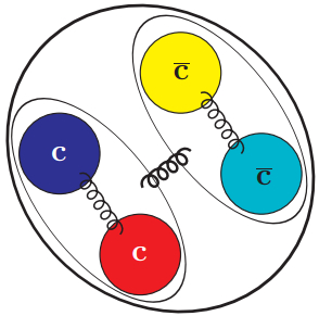
Figure 1.  (color online) Pictorial representation of the all-charm tetraquark in the diquark-antiquark scheme.

where κ_s, sometimes called the "color factor", is related to the color configuration of the system (it can be negative or positive), α_s is the QCD fine structure constant and b, sometimes called "string tension", is related to the strength of the confinement. One could also add a constant term, which would act as a zero-point energy.

Usually, in heavy quark bound states the kinetic energy of the constituents is small compared to their rest energy, hence a non-relativistic approach with static potentials can be a reasonable approximation. In two-body problems involving a central potential, it is convenient to work in the center-of-mass frame (CM), where one can use spherical coordinates to separate the radial and angular parts of the wavefunction, and the kinetic energy is written in terms of the reduced mass µ = (m₁ m₂)/(m₁ + m₂). We start with the time-independent Schrödinger equation:

We first solve this radial equation to obtain the energy eigenstate and the wavefunction of each particular state. Next, spin-dependent terms are included as perturbative corrections. They account for the splitting between states with different quantum numbers. Based on the Breit-Fermi Hamiltonian for one-gluon exchange [40-43], we introduce three spin-dependent terms: V_SS (spin-spin), V_LS (spin-orbit) and V_T (tensor). For equal masses m₁ = m₂ = m, they are given by:

where the radial-dependent coefficients come from the vector V_V and scalar V_S parts of the potential in Eq. (1),

where m is the constituent mass of the two-body problem (charm quark, or diquark). The second term in the spin-orbit correction (proportional to the scalar contribution) is a Thomas precession, which follows from the assumption that the confining interaction comes from a Lorentz scalar structure. Notice that if we introduce a constant term V₀ in the potential, it will not affect these radial coefficients, since only derivatives appear in them. In fact, adding a constant term only shifts the whole spectrum, forcing a change in the parameters such as to reproduce the charmonium spectrum, without actual improvement in the quality of the fit.

These spin-dependent terms are proportional to 1/m², which justifies their treatment as first-order perturbation corrections in heavy quark bound states. The expectation value of their radial-dependent coefficients can be calculated using the wavefunction obtained with the solution of the Schrödinger equation.

This framework appears frequently in quarkonium spectroscopy, but a better agreement between predicted states and the experimental data for $c\bar{c}$ mesons can be obtained by including the spin-spin interaction in the zeroth-order potential used in the Schrödinger equation (as done in Refs. [44-47]), with the artifact of replacing the Dirac delta by a Gaussian function which introduces a new parameter $\ell$. Then the spin-spin term becomes

When the term S₁·S₂ acts on the wavefunction it will generate a constant factor, so we still have a potential as a function only of the r coordinate. The expectation value of the operator of the spin-spin interaction can be calculated in terms of the spin quantum numbers using the following relation, $\langle {{\boldsymbol{S}}}_{1}\cdot {{\boldsymbol{S}}}_{2}\rangle =\;\langle \displaystyle \frac{1}{2}({{\boldsymbol{S}}}^{2}-\;{{\boldsymbol{S}}}_{1}{}^{2}-{{\boldsymbol{S}}}_{2}{}^{2})\rangle $, where S₁ and S₂ are the spins of particles 1 and 2 respectively, and S is the total spin in consideration.

The expectation value of the operator of the spin-orbit interaction can be calculated in terms of the quantum numbers of total angular momentum J (defined by the vector sum: J = L + S), total spin S, and orbital angular momentum $\ell$, using the following relation: $\langle {\boldsymbol{L}}\cdot {\boldsymbol{S}}\rangle =\;\langle \displaystyle \frac{1}{2}({{\boldsymbol{J}}}^{2}-{{\boldsymbol{L}}}^{2}-{{\boldsymbol{S}}}^{2})\rangle $. For S-wave states ($\ell$ = 0), the spin-orbit term $\left\langle {} \right.$L·S$\left. {} \right\rangle $ is always zero.

The tensor interaction demands a bit of algebra. For convenience, we redefine the tensor operator with an extra factor 12, which we remove from its radial coefficient in Eq. (8):

The results for the diagonal matrix elements of the tensor operator between two spin 1/2 particles, like in the mesons, can be found in Refs. [41, 48] and also (with more details) in Ref. [49]. The expectation value of the tensor is non-zero only for

After some manipulations of the spin operators, with the aid of some relations of spherical harmonics and the Pauli matrices with respective eigenvalues, we can obtain the following general result, which satisfies the above conditions (it always vanishes if $\ell$ = 0 or S = 0):

for any of the allowed values of J and $\ell$. For instance, for $\ell$ = 1 we have $\langle {{\boldsymbol{S}}}_{12}\rangle =-\displaystyle \frac{2}{5}, +2, -4$, for J = 2, 1, 0, respectively. These results are valid for diagonal matrix elements. The tensor actually has non-vanishing non-diagonal matrix elements, but as a first-order perturbation correction they can be neglected. They would be important if the tensor operator were to be used as part of the potential, which would cause the mixing of the wavefunction itself, as in the deuteron [50, 51].

Notice that in order to obtain these three general cases of non-vanishing diagonal matrix elements of the tensor operator for two spin 1/2 particles in Eq. (12), it is necessary to make use of a few relations that are valid only for Pauli matrices [48, 49], like its eigenvalues and the anticommutation relation. Therefore, we cannot use this result in the diquark-antidiquark tensor interaction (if we wish to treat it as a two-body problem), since the diquarks can have spin 0 or 1. This issue will be discussed later when we address the tetraquark interaction.

Regarding the wavefunction, we will consider only pure states where $\ell$ (orbital), S (total spin), and J (total angular momentum) are good quantum numbers. Then the wavefunction will be composed of a radial part and an angular part which comes from the coupling of spherical harmonics and spin functions at a specific value of J.

Solving the eigenvalue equation (2), one can obtain the interaction energy E and the wavefunction y(r) of the two-body system under consideration, where both depend on the number of nodes of the wavefunction n (or principal quantum number N = n + 1), on the orbital angular momentum number $\ell$, and in the case of the spin-spin correction included in V⁽⁰⁾, they will also depend on the total spin S and on the constituent spins S₁ and S₂. Since the Schrödinger equation has no analytical solution for the potentials that are relevant here, we solve it numerically, using an improved version of the code published in Ref. [52].

An interesting quantity that can be used to check the validity of the non-relativistic approximation is the velocity of the constituents in each of the systems in consideration: the quark velocity inside the meson or the diquark velocity inside the tetraquark. As discussed in Ref. [53], the mean square velocity can be obtained from the kinetic energy, which can be calculated directly from the Hamiltonian, or using the virial theorem:

where V⁽⁰⁾(r) is the effective zeroth-order potential placed in the Schrödinger equation and µ is the reduced mass:

Both methods yield approximately the same result within the numerical precision employed.

One interesting aspect of the non-relativistic approach is that, even though the charmonium system is not completely non-relativistic, a surprisingly good reproduction of its mass spectrum can be obtained. As discussed in Ref. [54], where a charmonium model is developed with completely relativistic energy and also with non-relativistic kinetic energy, good agreement with the experimental data can be obtained with both methods, just by using a different set of parameters in the effective potential employed.

The value of the square modulus of the wavefunction at the origin, |Ψ(0)|², is an important quantity. If the spin-spin interaction was treated as a first-order perturbation without the Gaussian smearing, it would be proportional to |Ψ(0)|² because of the Dirac delta. Decay widths can also be calculated using the wavefunction or its derivative at the origin. Only S-wave states ($\ell$ = 0) have non-zero value of the wavefunction at the origin. For states with orbital angular momentum ($\ell$ $ \ne $ 0), the centrifugal term in the Schrödinger equation creates a "centrifugal barrier", which makes the wavefunction at the origin vanish. Thus, for $\ell$ $ \ne $ 0 we will assume |Ψ(0)|² = 0 and for S-wave we have

In fact, the important quantity is the square modulus of the radial wavefunction at the origin, |R_{n, $\ell$}(0)|², which can be obtained directly from the numerical calculations. In the literature on quarkonium models, we find the following formula (see Ref. [41] for a deduction) that relates the wavefunction at the origin |Ψ(0)|² to the radial potential V⁽⁰⁾(r):

We have checked that the result obtained directly from the numerical method is compatible with the one obtained using the formula above.

In more sophisticated quarkonium models, such as the relativized potential model of Ref. [44], the coupling constant α_s is considered as a "running" parameter, that changes according to the energy scale of each bound state. However, we have chosen to adopt the non-relativistic model of Ref. [47], where α_s is as a constant in the potential, which is also a common approach in many charmonium models.

The values of α_s, the charm quark mass m_c, the string tension b, and the Gaussian parameter σ, will be obtained from a fit of the charmonium experimental data, and once the best set is found, they are kept fixed to generate the whole mass spectrum.

In order to get good estimates for diquarks and tetraquarks, we first study the spectrum of charmonium. In this case, the color factor κ_s in Eq. (1) should be that of a color singlet state, since for $c\bar{c}$ mesons we have $|q\bar{q}\rangle :3\otimes \bar{3}=1\oplus 8$ [55, 56]. The result for the color singlet is κ_s = -4/3 [49, 55].

After having solved the Schrödinger equation, the mass of a particular state will be given by:

The parity and charge conjugation quantum numbers of $q\bar{q}$ states are given by [55] P = (-1)^$\ell$+1 and C = (-1)^$\ell$+S repectively. Using the equation above we calculate the masses ${M}_{i}^{{\rm{calc}}}$ of the i states with well defined P and C, then we fit the experimentally measured masses ${M}_{i}^{\exp }$ and determine the parameters minimizing the χ², defined as:

Following Refs. [47, 54] we choose w_i = 1, which is equivalent to giving the same statistical weight to all the states used as input. This way we ensure the resulting set of parameters will simultaneously handle the spin-spin splitting in the S-wave, the spin-orbit and the tensor splitting, which are especially important in the P-wave, and the radial excitations as well.

In the study of tetraquarks, we shall treat the full four-body problem as three two-body problems. Repeating the steps described in the previous subsection, we first compute the mass spectrum of the diquark, then we do the same for the antidiquark and finally we solve the Schrödinger equation once again for a two-body system composed of the diquark and antidiquark. The inspiration for this factorization is the color structure behind it.

A diquark is a cluster of two quarks which can form a bound state. This binding is caused by one-gluon exchange between the quarks. In this interaction the factor κ_s can be negative, then the short distance part (∝ 1/r) of the potential will be attractive. The SU(3) color symmetry of QCD implies that, when we combine two quarks in the fundamental (3) representation, we obtain: $|qq\rangle :3\;\otimes \;3=\bar{3}\oplus 6$. Similarly, when we combine two antiquarks in the $\bar{3}$ representation, they can form an antidiquark in the 3 representation. Then the diquark and antidiquark can be combined according to $|[qq]-[\bar{q}\bar{q}]\rangle :\bar{3}\;\otimes \;3=1\;\oplus \;8$ and form a color singlet, for which the one-gluon exchange potential is also attractive (see Refs. [56-58]). The antitriplet state is attractive and yields a color factor κ_s = -2/3, while the sextet is repulsive and yields a color factor κ_s = +1/3 [49, 55]. Therefore we will consider only diquarks in the antitriplet color state. Indeed, for the single-flavor tetraquarks only the antitriplet diquarks can build pure states [27], while the sextet diquarks would necessarily appear mixed and in just a few cases. In Refs. [61, 62] the sextet contribution was found to be negligible in heavy tetraquarks with different flavor structure, like $ud\bar{b}\bar{b}$. Nevertheless, at the end of the presentation of our results, we will present and discuss results obtained with $6-\bar{6}$ configurations. We will use a diquark [cc] in the ground state, with no orbital nor radial excitations, such that we have the most compact diquark. We choose the attractive antitriplet color state, which is antisymmetric in the color wavefunction. Then, in order to respect the Pauli principle (the two quarks of the same flavor are identical fermions), the diquark total spin S must be 1. In this way the total wavefunction of the diquark will be antisymmetric.

Notice that going from the color factor -4/3 (for quark-antiquark in the singlet color state) to the color factor -2/3 (for quark-quark in the antitriplet color state) is equivalent to introducing a factor 1/2, which one would expect to be a global factor since it comes from the color structure of the wavefunction. Because of that, it is very common to extend this factor 1/2 to the whole potential describing the quark-quark interaction. This rule is motivated by the interactions inside baryons, where two quarks can also be considered to form a color-antitriplet diquark, which can then interact with the third quark and form a color-singlet baryon. Since this seems to give satisfactory results in baryon spectroscopy, it has also been extended to diquarks inside tetraquarks. The general rule would be simply ${V}_{qq}={V}_{q\bar{q}}/2$. Many authors with different tetraquark models, for instance Refs. [59, 60], also divide the confining part of the potential by 2 in order to adapt it to the diquark case. In our model, besides the change in the color factor, the string tension b, obtained from the fit of $c\bar{c}$ spectra, will be also divided by 2.

The calculation of the total mass of the diquark is completely analogous to the $c\bar{c}$ mesons, as in Eq. (17). The spin-dependent corrections are also analogous since we are still dealing with a two-body system composed of two spin 1/2 particles.

The all-charm tetraquark will be treated as a two-body (cc - $\bar{c}\bar{c}$) system with ${m}_{cc}={m}_{\bar{c}\bar{c}}$. The color factor should correspond to the color singlet, therefore we will use κ_s = -4/3 and also the same parameters α_s, b and σ obtained from the fit of the $c\bar{c}$ spectrum. The calculation of its total mass will also be analogous to the charmonium case:

In order to properly calculate the spin-dependent corrections we need to remember that the diquarks have spin 1. Then, for the coupling of a spin 1 diquark and spin 1 antidiquark, we will have the total tetraquark spin S_T = 0, 1, 2. Besides that, we will also allow radial and/or orbital excitations in the diquark-antidiquark system. In our non-relativistic approach, we use ordinary quantum mechanics to couple the total spin S_T to the orbital angular momentum L_T into the total angular momentum J_T.

For the spin-spin and spin-orbit corrections, we can obtain the angular factors from the spin, orbital and total angular momentum quantum numbers. However, for the tensor correction we only have a general result (in terms of eigenvalues) for the interaction between two spin 1/2 particles, shown in Eq. (12). Then, for a proper treatment of the tensor interaction in the diquark-antidiquark system we will explicitly apply the tensor operator on the angular part of the tetraquark wavefunction, as we will describe below.

Let us focus on the spatial and spin components of the wavefunction. We factorize the radial wavefunction from the angular one that combines orbital angular momentum and spin, which are coupled using Clebsh-Gordan coefficients. We will use the indices 1 and 2 for the two quarks inside the diquark, and 3 and 4 for the two antiquarks inside the antidiquark (see Fig. 2).

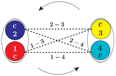
Figure 2.  (color online) Pictorial representation of the tensor interaction between diquark and antidiquark. The arrows represent the orbital angular momentum.

To illustrate our procedure to treat tensor interactions, we present one specific example with total spin S_T = 2, L_T = 1 and J_T = 2. S_d and ${S}_{\bar{d}}$ will denote the total spin of the diquark and antidiquark, respectively. We write the possible couplings in a generic form |S, M_S$\left. {} \right\rangle $, where S is the total spin and M_S is its z-component. The arrows denote the spins of each constituent, in the order 1, 2 for the diquark and 3, 4 for the antidiquark. As usual the up arrow denotes spin up, $\left.\left|\displaystyle \frac{1}{2},-\displaystyle \frac{1}{2}\right\rangle\right. $, and the down arrow denotes spin down, $|\displaystyle \frac{1}{2},-\displaystyle \frac{1}{2}\rangle $. We show it in terms of diquark and antidiquark spin basis, and also in terms of the two quarks and two antiquarks spin basis (each group of four arrows is always in the order "1234"). These wavefunctions were inspired by the ones presented in Refs. [45, 58, 61, 62], and we generalized them to include orbital angular momentum between diquark and antidiquark. For the choices mentioned above the wavefunction reads:

For L_T = 1 we have seven combinations to get J_T if we are considering spin 1 diquark and antiquark: one for S_T = 0 (J_T = 1), three for S_T = 1 (J_T = 0, 1, 2) and three for S_T = 2 (J_T = 1, 2, 3).

We now explicitly apply the tensor operator on the above angular wavefunction and we note that within our approximations, it is equivalent to apply this operator directly on the diquark-antidiquark pair (in spin 1 basis) or consider a sum of four tensor interactions between each quark-antiquark pair (spin 1/2 basis) as illustrated in Fig. 2, as would be expected from the angular momentum algebra¹⁾. We have:

1) To see this, we could write S_d = S₁ + S₂, ${{\boldsymbol{S}}}_{\bar{d}}={{\boldsymbol{S}}}_{3}+\;{{\boldsymbol{S}}}_{4}$ and open the tensor between diquark-antidiquark into four tensor operators between quark-antiquark pairs.

Since the tetraquark is treated as a two-body system, the expectation value of the radial wavefunction between every $q\bar{q}$ pair is the same and can be factorized. In a four-body problem (using Jacobi coordinates, for example) where all the four constituents are allowed to move and interact with each other at the same time, this would not be true. This type of approach can be found in other models of tetraquarks, for instance in Refs. [61, 62]. Usually in this kind of approach only the ground state is considered, with no orbital excitations, and hence only the spin-spin interaction is relevant, since the spin-orbit and tensor vanish for $\ell$ = 0. Besides, in order to tackle the four-body problem one needs to resort to a variational approximation with Gaussian trial wavefunctions or similar methods, therefore there will always be a compromise between the precision of the numerical solution and the reliability of the assumptions.

In order to deal with the generalization of the tensor interaction to the tetraquark case, we will rewrite the tensor in a form that allows us to recover the same results that we already know for the particular case of two spin 1/2 particles and that can also be used as a generalization to other cases, such as the interaction between two spin 1 diquarks. The operator S₁₂ in Eq. (10) is a "rank-2" tensor which can be written in terms of spin operators and spherical harmonics, as shown in textbooks [63]. An extensive discussion of this approach can be found in Ref. [49].

The following functional form does not use any particular relation or eigenvalues for spin 1/2 particles, only general properties of angular momentum elementary theory. One can write the unity vector $\hat{r}$ in spherical coordinates and the spin operators in Cartesian components. Then they can be rearranged into raising, lowering and z-component spin operators and spherical harmonics of $\ell$ = 2, and we can write:

where

With the expressions above we can take the expectation value of the tensor operator in the angular wavefunctions, as in Eq. (20), and use the selection rules of the spherical harmonics to find the non-vanishing terms.

To close this subsection, we discuss the tetraquark quantum numbers, as in Refs. [64, 65]. We can use the diquark-antidiquark basis to label the possible quantum numbers J^PC of the tetraquark. We shall use the following notation:

where S_d is the total spin of the diquark, ${S}_{\bar{d}}$ is the total spin of the antidiquark, S_T is the total spin of the tetraquark, assumed to come from the coupling ${S}_{d}\otimes {S}_{\bar{d}}$, L_T is the orbital angular momentum relative to the diquark-antidiquark system (in the two-body approximation), and J_T is the total angular momentum of the tetraquark, assumed to come from the coupling S_T ⊗ L_T. The general formulae for charge-conjugation and parity of the tetraquark are:

Since we are interested in the T_4c tetraquark, where the diquarks are composed of two charm quarks with spin 1 in the antitriplet color configuration, for the S-wave states we have the following possibilities:

Note that all the S-wave tetraquarks described above have positive parity. The introduction of the first orbital excitation will bring a factor (-1) in both parity and charge conjugation. Then all the P-wave states (with L_T = 1) will have odd parity and the opposite charge conjugation in comparison with the S-wave states. In Table 1 we list the J^PC quantum numbers of the 10 possibilities which we consider for the S-wave and P-wave all-charm tetraquarks built with spin 1 diquarks (also in accordance with Refs. [66] and [15]).

In this section we present the results of the calculations with the formalism outlined in the previous section. We use the following notation in our tables: the principal quantum number is N (N = 1 for the ground state, N = 2 for the first radial excitation and so on), $\ell$ is the orbital angular momentum, S is the total spin and J the total angular momentum. In spectroscopy notation the states are usually labeled by N^2S+1$\ell$_J, with $\ell$ = 0, 1, 2, 3, $ \ldots $, $ \to $, S, P, D, F, $ \ldots $, for example 1³S₁ for J/ψ.

In order to get good estimates of diquark and tetraquark properties, we first study the spectrum of the conventional charmonium states to observe how well we can fit the experimental data. In our model we considered the zeroth-order potential of the form Coulomb plus linear plus smeared spin-spin interactions. We separate the spin triplet (S=1) and spin singlet (S=0) before solving the Schrödinger equation. Using κ_s = -4/3, S₁ = S₂ = 1/2 and S = 0 or S = 1, we replace the operator S₁ · S₂ by the constant [S(S+1)-S₁(S₁+1) - S₂(S₂+1)]/2 and we find the wavefunction y(r) and the eigenvalue E. In Fig. 3 we show the zeroth-order potential for total spin 0 or 1. Later the spin-orbit and tensor corrections are included, splitting orbitally-excited states.

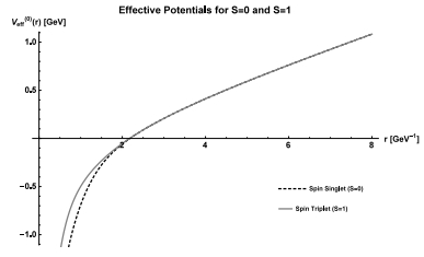
Figure 3.  Effective Potentials: Coulomb plus linear plus smeared spin-spin, for S = 0 and S = 1. Parameters are α_s = 0.5202, b = 0.1463 GeV², σ = 1.0831 GeV.

We performed a fit with experimental values from the PDG [67]. The four parameters were allowed to vary in the following range: 1.1 < m_c < 1.9 GeV, 0.1 < α_s < 0.7, 0.050 < b < 0.450 GeV², 0.7 < σ< 1.3 GeV. The results are also very similar to those from Refs. [46, 47], which were obtained with the fit of 11 $c\bar{c}$ states with equal statistical weight. We have included two more, h_c(1P) and χ_c2(2P), in a total of 13 states as input, obtaining the following values:

Several fits with different numbers of input states and alternative models were tested in Ref. [49]. There is one particular alternative case worth mentioning. In this case, we considered the spin-spin interaction as a first-order perturbation, proportional to the wavefunction at the origin, with the radial coefficient given by Eq. (6) (without the Gaussian smearing), and also removed the Thomas precession term from the spin-orbit interaction, which is proportional to the string tension b on Eq. (7). In this way the spin-dependent corrections come exclusively from the Breit-Fermi Hamiltonian describing one-gluon exchange, as in Ref. [43]. In this scheme it was possible to very accurately fit the 6 ground states 1S and 1P: η_c(1¹S₀), J/ψ (1³S₁), h_c (1¹P₁), χ_c0 (1³P₀), χ_c1 (1³P₁), χ_c2 (1³P₂), with the parameter set m_c = 1.2819 GeV, α_s = 0.3289 and b = 0.2150 GeV². This set is appealing since the mass of the charm quark is exactly the PDG value [67] obtained in the $\overline{MS}$ scheme, 1.28 $ \pm $ 0.03 GeV, and the coupling constant α_s is also smaller, favoring the assumption of the perturbative regime of QCD. However, for radial excitations, especially above the $D\bar{D}$ threshold, this scheme does not work very well and hence we restrict ourselves to the results obtained with the model that gives the best agreement with the whole experimental data set, since we believe this might yield better predictions for higher new charmonium states and also for the diquark and tetraquark.

In Table 2 we present the wavefunction properties. Notice that the inclusion of the spin-spin interaction in the zeroth-order potential creates a small difference between the wavefunction of the spin singlet and spin triplet. The spin 0 states receive a negative contribution from this interaction in the potential, which causes the short-distance region of the potential (small r coordinate) to be "more negative", generating states with smaller root mean square radius, higher value of the wavefunction at the origin, and higher quark velocity.

The spin-dependent interactions are very important in charmonium spectroscopy because they can test the QCD dynamics in the heavy quark context, lying between the perturbative and the non-perturbative regime. Particularly interesting is the role of the spin-spin interaction in orbitally-excited states. It is convenient to define the spin-average mass of a multiplet (spin here means J), also known as "center-of-weight" or "center-of-gravity" (c.o.g.):

For the P-wave ground state, for example, we have:

Interestingly, in the spin-average mass the spin-orbit and tensor corrections cancel each other and hence if the spin-spin correction is zero in the orbitally-excited singlet state (1¹P₁ for instance), its mass should be equal to this spin average. However, the spin-spin correction is zero for orbitally-excited states only if it is treated as a first-order perturbation proportional to the wavefunction at the origin. In our model, where we include the Gaussian term non-perturbatively, there will be a small difference. Therefore, in the present model the value of the mass M⁽⁰⁾ (before the splitting due to the orbital and tensor spin-dependent corrections) of the orbitally-excited states with total spin S = 1, like the 1³P, is equal to the c.o.g. of these states.

In Table 3 we present the results for the masses including the spin interactions. Note that the contribution of the spin-spin interaction to orbitally-excited states is not zero, especially in the P-wave, even though the wave function at the origin is still compatible with zero. Because of that the spin singlet in orbitally-excited states is slightly different from the spin-average (c.o.g.). The experimental measurements of 1P states suggest that they should be very close (see Table 4 for experimental values). As pointed out in Ref. [68], a precise measurement of the difference between the c.o.g. of the 1³P_J states and the singlet 1¹P₁ can provide useful information about the spin-dependent interactions in heavy quarks. Actually, the prediction for h_c(1¹P₁) is already close to the experimental value and even more so if one considers its mass as the spin-average of the ³P_J states (as done in Ref. [47] for the calculations where its mass was required). Also, the inclusion of the recently measured χ_c2(2P) [69, 70] did not affect the resulting set much, even though the prediction for its mass is a little higher than the experimental value.

In the 2014 edition of the PDG [71] the X(3915) was assigned as the 2³ P₀ $c\bar{c}$ state, the χ_c0(2P), but due to many reasons [72] it has been removed from this position. The X(3915) still has the status of an exotic resonance. A discussion about its nature (and also about the χ_c2(2P) state) can be found in Ref. [73]. A recent example of the X(3915) interpreted as a diquark-antidiquark tetraquark $[cs][\bar{c}\bar{s}]$ can be found in Ref. [74]. In Ref. [75] an analysis of Belle [69] and BaBar [70] data showed some evidence of the "real" χ_c0(2P) indicating that its mass could be around 3837.6$ \pm $11.5 MeV, which is in better agreement with quarkonium models. Recently, the Belle collaboration found a candidate for the χ_c0(2P) in the data of ${e}^{+}{e}^{-}\to J/\psi D\bar{D}$ [76], with a mass of ${3862}_{-32-13}^{+26+40}$ MeV and a width of ${201}_{-67-82}^{+154+88}$ MeV.

Finally, in Table 4 we compare the results of the model with the experimental data, which are illustrated in the mass spectrum presented in Fig. 4. We can see that the agreement with the experimental data is satisfactory.

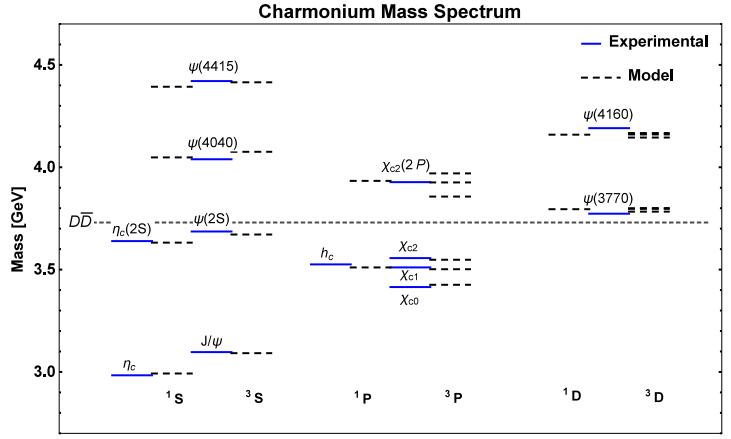
Figure 4.  (color online) Spectrum of charmonium. Solid lines: experimental data [67]. Dashed lines: results from the model. Parameters are m_c = 1.4622 GeV, α_s = 0.5202, b = 0.1463 GeV², and σ = 1.0831 GeV. Each state is shown with experimental data on the left and model results on the right. Notice that for some of the calculated states there is no experimental data to compare with.

We now present our calculations for heavy diquarks composed of two charm quarks cc (which are equivalent for antidiquarks $\bar{c}\bar{c}$ in our framework). We use the model for charmonium discussed in the previous subsection, except that due to the different color structure, the color factor is now κ_s = -2/3, which corresponds to the attractive antitriplet color state, and the string tension b will be half of that obtained for the $c\bar{c}$ charmonium mesons. We will adopt the parameter set obtained by fitting this model to 13 $c\bar{c}$ states.

In Tables 5 and 6 we present the results for the diquark wavefunctions and masses, respectively. For completeness we also show diquarks in the 1P, 2S and 2P states. Because of the restrictions due to the Pauli exclusion principle the possibilities are much less numerous. Also, since the P-wave introduces a (-1) factor in the parity, the antisymmetric restriction in the wavefunction implies that their total spin S should be 0 if they are in the antitriplet color state.

In Table 7 we show a few results from other works about cc diquarks. Due to differences in the models and presentation in each reference, we show only the information that can be compared to our results. In particular, we select only the results that correspond to the (attractive) antitriplet-color configuration. As can be seen, the 1S diquark is very similar in all the models, with a mass around 3.1 GeV.

As discussed above, the diquark-antidiquark tetraquark is treated as a two-body system. The diquark masses were presented in the previous subsection and the parameter set was obtained from a fit to the charmonium data. The tetraquark spectrum is calculated by replacing the charm quark mass by the diquark mass m_cc.

We now present the spectrum of the all-charm tetraquark considering the ground states 1S and the first orbital excitations 1P (relative to the diquark-antidiquark system), including all the possible combinations of total spin and total angular momentum. We also include the radial excitations 2S and 2P, in a total of 20 T_4c states built with two cc diquarks, each of them being in an antitriplet color state and spin 1 (1³S₁). These 20 states were built considering the coupling of the total spin of the tetraquark S_T (composed of the coupling of the total spins of the diquark S_d and antidiquark ${S}_{\bar{d}}$) with the relative orbital angular momentum L_T between diquark and antidiquark, resulting in a total angular momentum J_T of the tetraquark, in analogy to the $c\bar{c}$ charmonium spectrum. The corresponding parity and charge-conjugation quantum numbers of each combination are compiled in Table 1.

In our model the spin-spin interaction is treated non-perturbatively. In mesons and diquarks we had only two possibilities for total spin when combining two spin 1/2 particles S = 0, 1. Now, since we consider spin 1 diquark and antidiquark, we have three possibilities for total spin S_T = 0, 1, 2, and therefore three different zeroth-order potentials, and consequently three wavefunctions for each NL_T state, as presented in Table 8. The splitting structure from the perturbative corrections (spin-orbit and tensor) also has more possibilities, as presented in Table 9 with the masses of the 20 T_4c states. In Fig. 5 we show the mass spectrum.

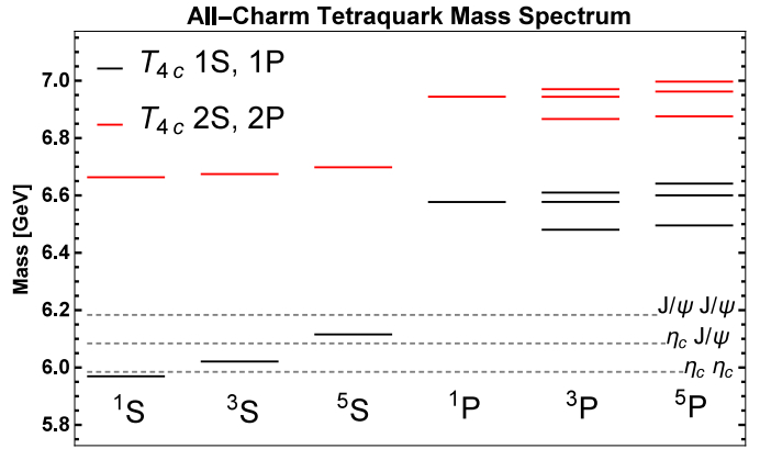
Figure 5.  (color online) Spectrum of T_4c obtained with the model, using ground state (1³S₁) diquark and antidiquark. Parameters are m_cc = 3133.4 MeV, α_s = 0.5202, b = 0.1463 GeV², and σ = 1.0831 GeV.

From Table 8 we can observe that the tetraquark is very compact. In fact, its $\left\langle {} \right.$r²$\left. {} \right\rangle $^1/2 is even smaller than the ground state diquark. This result apparently invalidates our initial assumptions, which implied a two-body diquark-antidiquark interaction where the (anti)diquarks are considered as point-like objects. However, the large diquark radius may just be an artifact of the Cornell-like potential used to describe the cc ($\bar{c}\bar{c}$) interaction. The result obtained only tells us that either the real cc interaction is not Cornell-like or that the diquark-antidiquark picture is not correct. Knowing that the diquark-antidiquark was successful in describing the recently observed multiquark states, we rather tend to question the Cornell-like potential (which was arbitrarily chosen) for this system. Indeed, there are calculations indicating that perhaps the dominant short-distance interaction between two quarks (or two antiquarks) is mediated by (non-perturbative) instantons and not (perturbative) one-gluon exchange. This interaction is attractive and strong in some channels (see for example, Ref. [9]). In the present work we choose to keep using the Cornell-like potential because we need to know the diquark mass to use it as input in the final two-body (diquark-antidiquark) problem. One could simply take the diquark mass as a free parameter and try to adjust it. However, obtaining it from the solution of the Schrödinger equation is a good strategy, at least from the practical point of view. The use of the Cornell potential for the quark-quark interaction is an elegant way to estimate the diquark mass, taking into account the diquark color structure in analogy to the $c-\bar{c}$ interaction, which successfully describes the charmonium spectrum. In fact, in Ref. [80], using this sequence of three two-body problems allowed the authors to successfully reproduce many properties of the already measured multiquark states. In the future the Cornell potential should be replaced by some more realistic quark-quark interaction. For now, we would like to use the obtained results and consider them as "privileged" guesses for the diquark masses.

As suggested in Ref. [15], the two-body approximation is better for orbitally-excited states, such as the P-wave considered here, since the centrifugal barrier would suppress overlap at the origin. As we can see in Table 8, the compactness of the T_4c is also reflected in the value of the wavefunction at the origin for the 1S states, which is very large.

In Table 9 we see that the compactness of the 1S states is mainly caused by the Coulomb interaction. This suggests that the one-gluon exchange is indeed the dominant mechanism responsible for the very strong binding between diquark and antidiquark, which causes the energy eigenvalue E to be negative. This also implies that the spin-spin interaction is strong. In this case we must have in mind that the factors coming from S₁ · S₂ are larger for the coupling of two spin 1 than for two spin 1/2 particles. It is interesting to see that even though the spin-dependent terms are now suppressed by a factor $1/{m}_{cc}^{2}$ and one would naturally expect them to be smaller when compared to the corresponding terms in $c\bar{c}$ mesons, the color interaction brings diquark and antidiquark so close that the suppression due to this factor is overwhelmed by the huge superposition at the origin of the system. The confinement term, on the other hand, increases its contribution as radial or orbital excitations are included, as in $c\bar{c}$ mesons.

In Fig. 5 we can see that the masses of the 20 states are concentrated in the range between 6 and 7 GeV. Among the 1S states, the lowest one, with J^PC = 0⁺⁺, lies very close to the η_c pair threshold. Within our uncertainties (both from the choice of parameters as well as the assumption of the diquark-antidiquark structure), we cannot say whether this state is below or above such a threshold. If it is above, it could be seen as a narrow state in the η_cη_c invariant mass. If it is below, then it would be stable against the rearrangement in $c\bar{c}$ pairs and other mechanisms would be necessary. Several possibilities are discussed in Ref. [30], with special attention to the 0⁺⁺ lowest state, such as ${T}_{4c}\to D\bar{D}$ through $c\bar{c}\to g\to q\bar{q}$. On the other hand, in Ref. [15] several decay possibilities of the orbitally-excited states are also discussed and branching fractions are estimated. It is interesting to see that even our estimates for the excited states with NL_T = 2S, 2P are below the threshold of decay into doubly-charmed baryon pairs due to light quark pair creation, $cc\bar{c}\bar{c}\to (ccq)+(\bar{c}\bar{c}\bar{q})$, which is above 7 MeV.

The second lowest state, with quantum numbers J^PC = 1^+-, could rearrange itself into η_cJ/ψ. However, this state seems to be more than 50 MeV below this two-meson threshold, and therefore it should be stable. The highest 1S state, with quantum numbers J^PC = 2⁺⁺, is also more than 50 MeV below the corresponding J/ψ pair threshold. It could still decay into $\ell$_c pairs in the D-wave, but this mechanism should be suppressed.

In order to be consistent with our $c\bar{c}$ results, in Fig. 5 the two-meson thresholds are shown using the values of charmonium masses obtained with our model, which were compared to the experimental values in Table 4. In Table 10 we compare all the 1S and 1P T_4c states with the corresponding lowest S-wave two-meson thresholds. We see that while the 1S states lie close to or below their thresholds, the orbitally-excited ones are close to or above the corresponding thresholds. Therefore, it would be interesting to search for these states in the two-meson invariant mass distributions, since some of them could show up as narrow peaks just around the threshold, like the 1^-- state (from the 1¹P₁ configuration) in the η_c(1S)h_c(1P) invariant mass at 6.50 GeV, the 2^-- (from the 1⁵P₂ configuration) in the J/ψ(1S) χ_c1(1P) invariant mass at 6.60 GeV, and the 3^-- state (from the 1⁵P₃ configuration) in the J/ψ(1S) χ_c2(1P) invariant mass at 6.65 GeV.

One of these orbitally-excited states is of particular interest, since it presents exotic quantum numbers that cannot be obtained as a simple $c\bar{c}$ system: the 1^-+ (from the 1³P₁ configuration). This state could be searched for in the η_c(1S) χ_c1(1P) invariant mass. However, it might be quite broad since our predictions show that it is about 80 MeV above its two-meson threshold.

Next, we comment on the results of other works which also investigate the existence and properties of this state composed of four charm quarks. Some of them also consider a sextet structure for the diquarks (which can also lead to a color singlet tetraquark). In the following tables we present a compilation of the main results.

First, we show the results of Ref. [2] in Tables 11 and 12. In this work a variational method with Gaussian trial wavefunctions was employed to study all-heavy tetraquarks, using a four-body coordinate system. The interactions were described with a potential due to the exchange of color octets in two-body forces. Two potentials were used: model I is a Cornell-type (Coulomb plus linear) and the model II is of the form A+Br^β. Also, a version of the MIT bag model was used with the Born-Oppenheimer approximation. Both color structures were considered, $\bar{3}-3$ and $6-\bar{6}$. S-wave and P-wave were considered with both potentials, and spin shifts were calculated with the Cornell-like potential.

In Table 13 we compile the results of Refs. [66, 78], where the T_4c production was studied. The estimates for the T_4c are very similar to those presented in this work. The authors used the diquark results of Ref. [77], where the cc diquark was calculated as a baryon constituent (we also compared these diquark results with ours). The same strategy of dividing the problem into two-body problems was used, but only S-wave states were calculated, and the spin-spin splitting was considered between each spin 1/2 constituent pair, using the wavefunction at the origin of the diquark or of the charmonium, depending on the interacting pair. It is interesting to see that the 0⁺⁺ state is very close to our result, and the 1^+- is also below the η_cJ/ψ threshold. However, the 2⁺⁺ is about 20 MeV above the J/ψ J/ψ threshold, indicating that this state could be seen in the J/ψ J/ψ invariant mass.

In Table 14 we compare our results for the S-wave T_4c with those of the recent diquark-antidiquark studies: those with antitriplet diquarks [66, 78], and those with the color-magnetic model [27] and with QCD sum rules [28].

In Table 15 we compare our results with the contribution of each term used to calculate the 0⁺⁺ T_4c in Ref. [30], which was based in meson and baryon masses. The constant V₀ is obtained as twice the constant term S obtained from the fit of baryon and meson masses (which is added only into baryon masses, related to the QCD string junction, as discussed in that reference). Remember that in our model the spin-spin interaction is contained in the energy eigenvalue.

Finally, in Table 16 we compare our results for the P-wave T_4c with the old diquark-antidiquark predictions of Chao [15], the recent diquark-antidiquark predictions of QCD sum rules [28] and with lattice results [24].

The use of the Cornell potential allows us to study the charmonium spectrum without the confining interactions, which can easily be "switched off" by choosing the string tension to be zero. We can thus repeat all our calculations and check whether we find bound diquark states and also a bound T_4c. We have done these calculations and we find both diquark and tetraquark bound states. The obtained diquark and T_4c ground states have masses equal to m_cc = 2881.4 MeV and T_4c = 5.3-5.4 GeV (for the lowest 1S states), respectively, as shown in the Appendix. These results can have applications in the context of relativistic heavy ion collisions, where a deconfined medium is formed (the quark-gluon plasma, QGP). Our results suggest that the T_4c can be formed and perhaps survive in the QGP phase.

The tetraquark composed of four quarks of the same flavor is constrained by the Pauli exclusion principle, which restricts the possibilities of the diquark wave function. The most favorable case is the one presented in the previous sections, where quarks in the diquark are in the attractive antitriplet color state (antisymmetric), in the ground state 1S with no orbital nor radial excitations (symmetric) and with total spin S = 1 (symmetric), resulting in an antisymmetric wave function appropriate for identical fermions. A diquark in the repulsive color sextet configuration (symmetric) should either have total spin S = 0 (antisymmetric) or have an internal orbital excitation. This excitation strongly disfavors the compactness of the diquarks, which underlies the assumption that the dynamics is dominated by one-gluon exchange. Therefore, any internal orbital excitation in the diquarks can be safely neglected, and we end up with two orthogonal building blocks: the antitriplet diquark with spin 1 and the sextet diquark with spin 0. There could be some mixing between these two states. We know that spin 0 diquarks can only form tetraquarks with total spin S_T = 0, therefore the tetraquarks composed of sextet diquarks would only mix with four of the 20 states presented in this work, i. e. the states 1S and 1P with quantum numbers J^PC = 0⁺⁺ 1^-- and both respective radial excitations. All the other states are necessarily composed of pure antitriplet diquarks, since to have spin 1 sextet diquarks one would need both diquark and antidiquark with one unit of internal orbital excitation, which is highly unlikely.

The exchange of one gluon between a quark inside the diquark and an antiquark inside the antidiquark could mix the color states $\bar{3}-3$ and $6-\bar{6}$. Unfortunately this cannot be implemented in the present model, where the four-body problem is factorized in subsequent two-body systems. The mixing can be taken into account in a full four-body problem, as done in Ref. [62], where both color configurations are present in the wave function from the beginning. However, in this reference, as well as in most of the works in the literature, the sextet configuration is found to be negligible when compared to the antitriplet configuration. In the composite wave function the $\bar{3}-3$ component completely dominates over the $6-\bar{6}$ one. This is essentially due to the repulsion inside the sextet diquark. The conclusion that we can draw from this observation is that even though the $\bar{3}-3$ and $6-\bar{6}$ can mix, a proper four-body approach reveals that they behave essentially as two independent states. The $6-\bar{6}$ contribution to the $\bar{3}-3$ is expected to be negligible, and the former should be calculated separately as a pure $6-\bar{6}$ state.

Let us now present results for the pure $6-\bar{6}$ tetraquark. In our model, we need first to compute the mass of the sextet diquark and then calculate the tetraquark spectrum. The color factor κ_s of the Coulomb term in the potential corresponding to the sextet configurations is +1/3. The string tension b of the linear confining term is the value taken for the charmonium divided by four, and its sign also changes. This interaction is completely repulsive and clearly cannot yield a bound state. However, one might argue that for non color-singlet configurations the long distance part of the potential is not well known and might be confining. We may get a rough estimate of the sextet diquark mass as being twice the charm quark mass. The spin of the diquark is zero (and so is the spin of the tetraquark) and hence all the spin-dependent interactions vanish. The interaction between a 6 diquark and a $\bar{6}$ antidiquark is very attractive. The color factor is -10/3, and the string tension is positive and a factor 10/4 larger than that of charmonium. Using these parameters we can estimate the mass of the $6-\bar{6}$ tetraquark in the four cases where it could mix with the $\bar{3}-3$ state. They are shown in Tables 17 and 18. We see that for the ground state we obtain an extremely bound state around 4 GeV. This might be an indication that the two-body approximation is already unrealistic and we should take into account the finite size of the diquarks. If we use a heavier diquark mass obtained with a confining string tension (about 3.2 GeV, 70 MeV above the antitriplet diquark) we again find an extremely bound ground state, since increasing the diquark mass reduces the tetraquark size, increasing the contribution of the attractive Coulomb term (as happens when we move from charmonium to bottomonium).

Before concluding we would like to add a remark on the scale dependence of our results. The one-loop QCD running coupling is given by:

In this formula the scale Q² is an input. It is a choice which defines the energy scale that is relevant to the problem. In our case we have used it as a constant, which was the same for the two-body $c\bar{c}$ problem and for the $cc-\bar{c}\bar{c}$ two-body problem. We have here ignored the effects of the running coupling. In principle, we could have chosen two different scales. For the $c\bar{c}$ problem it should be ${Q}^{2}\simeq {m}_{c}^{2}\simeq {(1.4)}^{2}$ GeV² and for the $cc-\bar{c}\bar{c}$ problem it should be ${Q}^{2}\simeq {m}_{cc}^{2}\simeq {(3.1)}^{2}$ GeV². Using these numbers in the above formula we obtain α_s(m_c) ~ 0.5 and $\ell$_s(m_cc) ~ 0.35. Changing the scale, the running coupling is reduced by approximately 30%. Using 0.35 instead of 0.5 changes the resulting masses of the bound states which come from the solution of the Schrödinger equation. However, this change is only 5% for the lowest lying (1S) state. For the higher states, i.e. the radial and orbital excitations, the effects of the running coupling are even smaller, because the distance between the two bodies is larger and the QCD-Coulomb interaction is less important. In this region the uncertainties in the string tension are dominant. We have checked that in the least favorable case (of a radial together with an orbital excitation) for a diquark-antidiquark calculation, changing the string tension by ~30% leads to changes in the final T_4c mass of $ \simeq $ 3%.

An alternative way to compute running coupling effects was described in Ref. [81], where the authors compare (using their formula 2.23) α_s in bottomonium with α_s in charmonium with a simple formula. Adapting their formula to our context, it reads:

which then leads to the same results quoted above. The observation made above suggests that we should correct our tables, changing the masses. Moreover, to be more accurate we should also take into account the uncertainty in the scale choice, e.g., considering ${Q}^{2}=\displaystyle \frac{{m}_{c}}{2}$, m_c, 2m_c and similarly for the diquark-antidiquark case. However, we feel that this analysis would also imply a global uncertainty analysis, which is beyond the scope of the present work. When dealing with very precise theoretical predictions, all results should contain the theoretical errors, which reflect the uncertainties in the calculations. This could be done in the present work by studying the effects caused by changing the masses, couplings and string tension. The uncertainty analysis could be improved by also including relativistic corrections (a cubic term in the kinetic energy). However, this degree of precision would be more appropriate when experimental data is available, allowing further constraints in the model, and it should be postponed for future work.

This was the first calculation of the T_4c spectrum with a non-relativistic diquark-antidiquark model. It was meant to check whether this approach reproduces what we know from the lattice calculations, from QCD sum rules and from the results of the Bethe-Salpeter approach. In this sense it is a preliminary calculation which we believe has passed the test. Further improvement could be made in the future by including a systematic analysis of the uncertainties, moving towards "precision physics". The real novelty of this work would be the power to identify the components of the masses and determine the role of the spin interactions, which are very difficult to isolate in the lattice and in QCD sum rules calculations.

In this work we first updated the Cornell model, (a very well known and accepted model for charmonium), obtaining a satisfactory reproduction of the charmonium spectrum, including the most recently measured states. We then extended this model to study the all-charm tetraquark ($c\bar{c}c\bar{c}$).

We explored a diquark-antidiquark configuration, including P-wave tetraquarks, and we extended the spin-dependent interactions between diquarks, including a consistent strategy to deal with the tensor interaction between two objects of spin 1. The fact that our model is relatively simple compared to the four-body approach and to the relativistic models allows us to study many of the T_4c properties with clarity, especially the role of the spin interactions.

We were able to study the behavior of the all-charm tetraquark when radial and orbital excitations are included, investigating the contribution of the one-gluon exchange, the confinement and the spin-dependent interactions, providing for the first time detailed results which elucidate the dynamics of the diquark-antidiquark structure.

The inclusion of one orbital excitation in the tetraquark also leads to a significant increase in the possibilities of quantum numbers and to the prediction of the exotic state with J^PC = 1^-+. The orbitally-excited $c\bar{c}$ states, having specific masses and quantum numbers, have different decay channels, which may be investigated experimentally.

Our model is simple and instructive, especially in what concerns spin interactions. For the lowest T_4c states our predictions are compatible with those made with other approaches. For the higher states, in particular those with orbital excitations, we make novel predictions which can be tested. In this region our predictions are more reliable, since the diquark-antidiquark spatial separation is bigger.

Our results and the others found in the recent literature on the T_4c tetraquark, taken together, should encourage a careful experimental search for these states at LHCb and Belle Ⅱ.

In Table A1 we show the results for the lowest 1S tetraquark states where both diquark and tetraquark were calculated without the linear confinement term and hence the only interaction is one-gluon exchange.

These 1S states are deeply bound. As we can see in Table A1, the binding energy for the lowest state, with J^PC = 0⁺⁺, is larger than -400 MeV, where about 100 MeV come from the spin-spin interaction. The resulting mass of 5.3 GeV is compatible with the results of Ref. [23], where a state with a dominant η_cη_c component and mass 5.3 $ \pm $ (0.5) GeV was found.

For the excited tetraquark states 2S, 1P and 2P, the binding energy is around -90 MeV and the spin-dependent interactions are of the order of 10 MeV, with masses around 5.6-5.7 GeV.