


 Abstract
 HTML
HTML Reference
 Related
 PDF
PDF


HTML
-
The idea of hadronic molecules is largely motivated by the existence of the deuteron as a bound state of a proton and neutron. For a recent review, see [1]. Thus, any development in nuclear physics could have an impact on hadron physics. An example would be the triton, which is a bound state consisting of three nucleons. This raises the question of whether there exist hadronic molecules formed of three hadrons. Another hint from nuclear physics is the existence of a possible kaonic nuclear bound state.The strong attraction of the
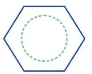
$\bar{K}N$ systems leads to the bound state Λ(1405) [2-10], and especially to its two-pole structure, as reviewed by PDG [11]. This has led to speculations concerning deeply-bound kaonic states in light nuclei, i.e.,$\bar{K}NN$ .The confirmation of such a kaonic light nuclei in the${}^{3}{\rm{He}}({{\rm{K}}}^{-}, \Lambda {\rm{p}})n$ process by the E15 Collaboration [12, 13] adds further motivation for both nuclear and hadronic physicists to consider three-body bound states. It also indicates that there could be three-body bound states formed by three hadrons. Several similar studies on three-body systems in hadron physics have been performed based on a quasi-two-body scattering approximation, such as the ψ′π+π− [14],$\phi K\bar{K}$ [15],$KK\bar{K}$ [16],${f}_{0}(980)\pi \pi $ [17],$J/\psi K\bar{K}$ [18],$DKK(\bar{K})$ [19],$BD\bar{D}$ , BDD [20],${B}^{(* )}{B}^{(* )}{\bar{B}}^{(* )}$ [21], KX(3872), KZc(3900) [22],${B}^{* }{B}^{* }\bar{K}$ [23], and${D}^{* }{D}^{* }{\bar{D}}^{(* )}$ [24] mesonic systems and the DNN [25], NDK,$\bar{K}DN$ ,$ND\bar{D}$ [26], and$N\bar{K}K$ [27] baryonic systems. We focus on the${D}^{(* )}{D}^{(* )}K$ system, which is a simple extension of the$\bar{K}NN$ system resulting by replacing the nucleons with charmed mesons. The advantage of this three-body system is that the dynamics of its two-body sub-system are well constrained by the current experimental data.To leading order, the behavior of three constituents sharing one virtual pion is similar to the idea of the delocalized π bondfor the formation of benzene in molecular physics, as illustrated in Fig. 1. We deal with the three-body problem in coordinate space by solving the Schrödinger equation, because one can directly extract the size of the bound state, which could be utilized as a criterion for whether hadrons represent the effective degrees of freedom.

Figure 1. (color online) A simplified illustration of a benzene ring as a hexagon, with a circle describing the delocalized π bond inside.
In this work, we solve the three-body Schrödinger equation to study whether there exists a bound state for the DD*K system1). As the kaon mass is considerably smaller than those of the charmed mesons, the Born-Oppenheimer (BO) approximation can be applied to simplify this case, although this involves an uncertainty of the order
${\mathcal{O}}({m}_{K}/{m}_{{D}^{(* )}})$ . The procedure is divided into two steps. First, we keep the two heavy mesons, D and D*, at a given fixed location R and study the dynamical behavior of the light kaon. In the next step, we solve the Schrödinger equation of the DD* system with the effective BO potential arising from the interaction with the kaon.1) In principle, all the channels with the same quantum number should couple with each other. However, in our case, because the binding energy of the two-body subsystem is approximately 40 MeV and the corresponding binding momentum γ is approximately 150 MeV, the interaction through the one-meson exchange diagram scales on the order of
${\mathcal{O}}({\gamma }^{2}/{m}_{E}^{2})$ , with mE being the mass of the exchanged meson. As a result, interactions with an exchanged meson other than the pion will be suppressed. Transitions among DsD*π, DDs*π, and DD*K occur either through K or K*, which is suppressed compared to the one-pion-exchanged potential. Thus, the DsD*π and DDs*π channels are not included in our calculation.In our case, as the typical momentum is approximately 150 MeV, a diagram with the mass of the exchanged particle being higher than the pion can be considered as a short-ranged contribution. Thus, we only consider the pion-exchange potential. Note that the two-pion-exchange (TPE) diagrams (Figs. 2(d) and (e)) comprise the next-to-leading order contribution, similar to that in nuclear physics. See, for example, [28-30] for reviews. Thus, we only consider the leading order one-pion-exchange (OPE) diagrams, i.e., those in Figs. 2(a), (b), and (c). This situation is analogous to the delocalized π bond in molecular physics. This is because there is only one virtual pion shared by the three constituents, as shown in Figs. 2(a), (b), and (c), instead of localizing between any two of them. We also note that it is important to consider these diagrams together. In this sense, this behavior is similar to that when three pairs of electrons are shared by the six carbon atoms in benzene. As a result, we work within the framework that respects SU(2) flavor symmetry2). The relevant Lagrangian is
2) The Lagrangian in Ref. [31] is invariant under the SU(3) symmetry when the interactions of DK and D*K are the same to the leading order.

Figure 2. Diagrams (a), (b), and (c) show the leading one-pion-exchange (OPE) diagrams for the transitions among the relevant three-body channels, i.e., the DD*K, DDK*, and D*DK channels. These three channels are labeled as the first, second, and third channels, respectively. Thus, the diagrams (a), (b), and (c) represent the transition potentials V12, V23, and V13, respectively. The (double) solid dashed lines represent the D(*) and K(*) fields. The dotted lines denote pion fields. The two-pion-exchange (TPE) diagrams, (d) and (e), comprise the next-to-leading order contributions.
$ \begin{eqnarray*}\begin{array}{ll} {\mathcal L} &=-{\rm{i}}\frac{2{g}_{P}}{{F}_{\pi }}\bar{M}{P}_{b}^{* \mu }{\partial }_{\mu }{\phi }_{ba}{P}_{a}^{\dagger }+{\rm{i}}\frac{2{g}_{P}}{{F}_{\pi }}\bar{M}{P}_{b}{\partial }_{\mu }{\phi }_{ba}{P}_{a}^{* \mu \dagger }\\ &\quad +\frac{{F}_{\pi }^{2}}{4}\langle {\partial }_{\mu }U{({\partial }^{\mu }U)}^{\dagger }\rangle +\frac{{F}_{\pi }^{2}}{4}\langle {\mathcal M} {U}^{\dagger }+U{ {\mathcal M} }^{\dagger }\rangle \end{array}\end{eqnarray*} $
where
$U=\exp ({\rm{i}}\phi /{F}_{\pi })$ with$ \begin{eqnarray}\phi =\left(\begin{array}{cc}\frac{{\pi }^{0}}{\sqrt{2}}&{\pi }^{+}\\ {\pi }^{-}&-\frac{{\pi }^{0}}{\sqrt{2}}\end{array}\right).\end{eqnarray} $
(1) and P(*) = (D(*)0, D(*)+) or
$({K}^{(* )-}, {\bar{K}}^{(* )0})$ . The last two terms in the Lagrangian above comprise the pion propagator. Here,$\bar{M}=\sqrt{{M}_{P}{M}_{{P}^{* }}}$ is the difference between the normalization factor for the relativistic and non-relativistic fields. The effective couplings gD = 0.57 (gK = 0.88) can be extracted from the partial width of the${D}^{* }\to D\pi $ (${K}^{* }\to K\pi $ ) process. This coupling for the bottom sector is taken to have the same value as that in the charm sector, which is consistent with the recent lattice result [32] to within 10%. As there is no direct OPE diagram for the D*K channel, an additional channel DK*1) is included as an intermediate channel. Because the three-momentum pK of the D*K system at the DK* threshold is 61% of its reduced mass μD*K, the relativistic effect of the kaon is not negligible. This is the reason why we employ the relativistic form of the interaction, and keep the expression for the kaon to the order${\mathcal{O}}(\frac{{p}_{K}}{{m}_{K}})$ . To take the substructure for each pion vertex into account, we adopt a monopole form factor$ {\mathcal F} (q)=\frac{{\Lambda }^{2}-{m}_{\pi }^{2}}{{\Lambda }^{2}-{q}^{2}}$ , with q being the four-momentum of the pion and Λ the cutoff parameter. With the cutoff ΛD*K = 803.2 MeV, we find a D*K bound state with a mass corresponding to the Ds1(2460). The dynamics of the$I=\frac{1}{2}$ DD*K system with an isosinglet D*K do not depend on the cutoff parameter for the DD* system, whose attractive and repulsive parts are precisely cancelled [33]. The DK subsystem cannot interact with each other through the OPE, even after considering the coupled channel effect.1) The reason for the D*K* channel not being included is that it is the next higher threshold.
The BO approximation is based on the factorized wave function
$ \begin{eqnarray}|{\Psi }_{T}(\mathit{\boldsymbol{R}}, r)\rangle =|\Phi (\mathit{\boldsymbol{R}})\Psi (\mathit{\boldsymbol{r}}_{1}, \mathit{\boldsymbol{r}}_{2})\rangle, \end{eqnarray} $
(2) with the two charmed mesons and the light kaon located at ± R/2 and r, respectively. Here, r1 = r+R/2 and r2 = r-R/2 are the coordinates of the kaon relative to the first and second interacting D*, respectively. In our case, owing to the OPE potential the three channels DD*K, DDK*, and D*DK are coupled with each other, as shown in Figs. 2(a), (b), and (c). The wave function of the kaon in the DD*K system is the superposition of the two two-body subsystems
$ \begin{eqnarray*}\begin{array}{ll}|\Psi (\mathit{\boldsymbol{r}}_{1}, \mathit{\boldsymbol{r}}_{2})\rangle &={C}_{0}\{\psi (\mathit{\boldsymbol{r}}_{2})\, |D{D}^{\ast }K\rangle +\psi (\mathit{\boldsymbol{r}}_{1})\, |{D}^{\ast }DK\rangle \\ &\quad +C[{\psi }^{^{\prime} }(\mathit{\boldsymbol{r}}_{1})+{\psi }^{^{\prime} }(\mathit{\boldsymbol{r}}_{2})]|DD{K}^{\ast }\rangle \}\, .\end{array}\end{eqnarray*} $
The constant C0 can be fixed by the normalization constraint of the total wave function. The wave functions ψ(ri) and ψ′(ri) of the two-body subsystems D*K and DK* are obtained by solving Schrödinger equation with these two channels coupled with each other.
In the BO approximation, the three-body Schrödinger equation can be simplified into two sub-Schrödinger equations [33]. One is the equation for the kaon,
$ \begin{eqnarray}H(\mathit{\boldsymbol{r}}_{1}, \mathit{\boldsymbol{r}}_{2})|\Psi (\mathit{\boldsymbol{r}}_{1}, \mathit{\boldsymbol{r}}_{2})\rangle ={E}_{K}(R)|\Psi (\mathit{\boldsymbol{r}}_{1}, \mathit{\boldsymbol{r}}_{2})\rangle \end{eqnarray} $
(3) at any given R with
$ \begin{eqnarray*}H(\mathit{\boldsymbol{r}}_{1}, \mathit{\boldsymbol{r}}_{2})=\left(\begin{array}{ccc}{T}_{11}(\mathit{\boldsymbol{r}}_{1}, \mathit{\boldsymbol{r}}_{2})&{V}_{12}(\mathit{\boldsymbol{r}}_{2})&0\\ {V}_{21}(\mathit{\boldsymbol{r}}_{2})&\delta M+{T}_{22}(\mathit{\boldsymbol{r}}_{1}, \mathit{\boldsymbol{r}}_{2})&{V}_{23}(\mathit{\boldsymbol{r}}_{1})\\ 0&{V}_{32}(\mathit{\boldsymbol{r}}_{1})&{T}_{33}(\mathit{\boldsymbol{r}}_{1}, \mathit{\boldsymbol{r}}_{2})\end{array}\right).\end{eqnarray*} $
Here, Tii is the relative kinetic energy for the K in the ith channel, and δM = MD+MK*-MD*-MK is the mass gap between the DDK* and DD*K (D*DK) channels. The explicit forms of the kinetic terms and the potentials can be found in App.. The parameter C can be determined using the variational principle ∂EK(R)/∂C = 0. The other sub-Schrödinger equation, for the two heavy charmed mesons, is
$ \begin{eqnarray}{H}^{^{\prime} }(\mathit{\boldsymbol{R}})|\Phi (\mathit{\boldsymbol{R}})\rangle =-{E}_{3}|\Phi (\mathit{\boldsymbol{R}})\rangle \end{eqnarray} $
(4) with
$ \begin{eqnarray*}\begin{array}{ll}{H}^{^{\prime} }(\mathit{\boldsymbol{R}})&={T}_{h}(\mathit{\boldsymbol{R}})+{V}_{h}(\mathit{\boldsymbol{R}})+{V}_{{\rm{BO}}}(\mathit{\boldsymbol{R}})\\ &=\left(\begin{array}{ccc}{T}_{D{D}^{\ast }}(\mathit{\boldsymbol{R}})&0&{V}_{13}(\mathit{\boldsymbol{R}})\\ 0&{T}_{DD}(\mathit{\boldsymbol{R}})&0\\ {V}_{31}(\mathit{\boldsymbol{R}})&0&{T}_{D{D}^{\ast }}(\mathit{\boldsymbol{R}})\end{array}\right)\\ &+{V}_{{\rm{BO}}}(\mathit{\boldsymbol{R}})\end{array}\end{eqnarray*} $
where VBO(R)=EK(R)+EB is the BO potential provided by the kaon, and EB is the binding energy of the isosinglet D*K system. The total energy of the three-body system relative to the DD*K threshold is E=-(E3+EB). The explicit forms of TDD*(R), TDD(R), V13(R), and V31(R) can be found in App..Because the three-body force only appears at next-to-leading order, which is neglected here, the dynamics of the three-body system can be described by those of its two-body sub-systems. Because the potential of the isospin singlet (triplet)D*K is attractive (repulsive), only the three-body DD*K system with the total isospin
$\frac{1}{2}$ and the isosinglet D*K can form a bound state:$ \begin{eqnarray*}\begin{array}{c}|D{D}^{* }K{\rangle }_{\frac{1}{2}, \frac{1}{2}}=\frac{1}{\sqrt{2}}[|{D}^{+}{(}_{{D}^{\ast +}}\rangle +|{D}^{+}{(}_{{D}^{\ast 0}}\rangle ], \\ |D{D}^{* }K{\rangle }_{\frac{1}{2}, -\frac{1}{2}}=\frac{1}{\sqrt{2}}[-|{D}^{0}{(}_{{D}^{\ast +}}\rangle -|{D}^{0}{(}_{{D}^{\ast 0}}\rangle ], \end{array}\end{eqnarray*} $
where the subscripts denote the isospin and its third component. How deep this is depends on how strong the D*K attraction is. Fig. 3(a) shows the dependence of the energy E3 for DD*K of the
$I({J}^{P})=\frac{1}{2}({1}^{-})$ system on the binding energy EB of its isosinglet two-body D*K system. The analogous bottom system is illustrated in Fig. 3(b). The two vertical bands in Fig. 3 represent the binding energies of D*K and${B}^{* }\bar{K}$ in Ref. [34], which allows one to deduce the energies E3 of the two systems
Figure 3. (color online) The binding energy of the DD*K three-body system with I = 1/2 in terms of that of the isosinglet D*K two-body system is presented in the left panel, as defined in Eq. 3. The uncertainty is estimated as mK/(2μDD*). The right panel shows the corresponding dependence for the
$B{B}^{* }\bar{K}$ system. The red point indicates the critical point, which represents the lower limit of the required binding energy of the isosinglet D*K or${B}^{* }\bar{K}$ to form a three-body bound state. The vertical dashed lines and bands represent the central values and uncertainties of the binding energies of the two-body subsystems from the chiral dynamics analysis [34].$ \begin{eqnarray*}{E}_{I=1/2}^{D{D}^{* }K}={8.29}_{-3.66}^{+4.32}\, {\rm{MeV}}, {E}_{I=1/2}^{B{B}^{* }\bar{K}}={41.76}_{-8.49}^{+8.84}\, {\rm{MeV}}, \end{eqnarray*} $
where the uncertainties are estimated as mK/(2μDD*) and mK/(2 μBB*), as discussed above. That means that after including the binding energies of the D*K and
${B}^{* }\bar{K}$ subsystems, there are two bound states with masses${4317.92}_{-4.32}^{+3.66}\, {\rm{MeV}}$ and${11013.65}_{-8.84}^{+8.49}\, {\rm{MeV}}$ , respectively. The critical point in Fig. 3 refers to the case that when the binding energy of D*K or${B}^{* }\bar{K}$ is larger than that value, a three-body bound state begins to emerge.The corresponding root-mean-square radii for each two-body subsystem are shown in Figs. 4 and 5 for the charm and bottom sectors, respectively.The root-mean-square between K and D(*) is 1.14 fm. The value for DD* is 1.65 fm. Both of these are of the order
$\hslash c/{m}_{\pi }1.41\, {\rm{fm}}$ , which characterizes the size of the state bound by the OPE1).Because the S-wave component dominates the isosinglet D*K wave function, the kaon is distributed evenly on an ellipse (grey dashed line in Fig. 4), with a root-mean-square radius of 0.79 fm on the plane perpendicular to the DD* direction. The case for the bottom sector is similar, as shown in Fig. 5. The root-mean-square radius between the kaon and bottom mesons is 0.96 fm. The distance between a pair of bottom mesons is 0.65 fm, which indicates that the kaon is distributed on a circle, with a root-mean-square radius of 0.90 fm on the plane perpendicular to the BB* direction. All of the above root-mean-square radii are sufficiently large to separate the two relevant constituents, making hadrons the effective degrees of freedom. In particular, although the root-mean-square radius between BB* is as small as 0.65 fm, it is still significantly larger than twice the Compton wavelength of the bottom meson.1) One should note that the typical size for the vector meson exchange potential is ħc/mρ∼0.26 fm, which is even smaller than the size (0.47 fm) of J/ψ [35]. In this case, hadrons can no longer be viewed as the effective degrees of freedom. In other words, the vector meson-exchanged potentials are part of the unknown short-distance contributions, which are of higher order from the effective field theory point of view, and require data to fix the corresponding coupling constants. This short-distance contribution is effectively modeled by the form factor that was introduced earlier.

Figure 4. (color online) Formation of the three-body DD*K bound state through the delocalized π bond (orange long-dashed curve). The root-mean-square radius of each two-body subsystem is explicitly indicated. The kaon is evenly distributed on the grey dashed ellipse.
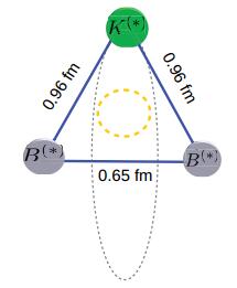
Figure 5. (color online) The same as Fig. 4, but for the
$B{B}^{* }\bar{K}$ system.The kaon energy in the three-body system defined in Eq. 3 is shown in Fig. 6, in terms of the distance between the two heavy mesons. When the distance goes to infinity, this returns to the binding energy of the two-body subsystem. Furthermore, when the charmed (bottomed) system gains another 42.29 MeV (42.19 MeV) of energy, the three-body system will totally break up into three individual particles. The dependence of the bottom system (blue dashed curve) is narrower but deeper, which means that its size is smaller, but its binding energy is larger. This is consistent with what we obtained above.

Figure 6. (color online) The kaon energy in the three-body system as a function of the distance R between two heavy-light mesons. The red dotted and blue dot-dashed horizontal lines represent the binding energies of the isosinglet D*K and
${B}^{* }\bar{K}$ systems, respectively. When the distance R is larger than a certain value, the kaon energy of the three-body system is equal to the binding energy of either the isosinglet D*K or${B}^{* }\bar{K}$ two-body system. The two-body binding energies are from Ref. [34].The long-distance DD*(D*K) potential from the OPE is related to that of the
$D{\bar{D}}^{* }({\bar{D}}^{* }K)$ potential by G-parity [36], i.e., the corresponding potentials V12(r2), V23(r1) and V13(R) change sign. As all of these are off-diagonal elements in the Hamiltonian, their signs do not affect the eigenvalues, but only affect the interference pattern of different components in the final physical wave function. Thus, there could also exist a three-body$D{\bar{D}}^{* }K$ bound state with the same binding energy. However, this introduces the additional uncertainty${m}_{\pi }^{2}/(2{\mu }_{D{D}^{* }})$ (which characterizes the natural energy scale of the OPE [37]), stemming from the unknown short-distance interaction, which is considered as the next-leading order contribution. Thus, for the$D{\bar{D}}^{* }K$ and$B{\bar{B}}^{* }\bar{K}$ system, the three-body binding energies are$ \begin{eqnarray*}{E}_{I=1/2}^{D{\bar{D}}^{* }K}={8.29}_{-6.13}^{+6.55}\, {\rm{MeV}}, \, {E}_{I=1/2}^{B{\bar{B}}^{* }\bar{K}}={41.76}_{-8.68}^{+9.02}\, {\rm{MeV}}\end{eqnarray*} $
with the additional uncertainty arising from the missing short-distance interaction. These correspond to two bound states with masses
${4317.92}_{-6.55}^{+6.13}\, {\rm{MeV}}$ and${11013.65}_{-9.02}^{+8.68}\, {\rm{MeV}}$ . The coincidence of the positions of the DD*K ($B{B}^{* }\bar{K}$ ) and$D{\bar{D}}^{* }K$ ($B{\bar{B}}^{* }\bar{K}$ ) systems is because only the leading-order OPE is considered in the calculation.Our result for the$D{\bar{D}}^{* }K$ system agrees with the value 4337.0-i3.3 MeV predicted in [22] within 3σ after considering the vector meson-exchanged potentials. This gives further support to the assertion that the vector meson-exchange potentials are higher order short-distance contributions.For the I = 1/2
$D{\bar{D}}^{* }K$ three-body bound state$ \begin{eqnarray*}\begin{array}{l}|D{\bar{D}}^{* }K{\rangle }_{\frac{1}{2}, \frac{1}{2}}=\frac{1}{\sqrt{2}}[-|{D}^{+}{(}_{{\bar{D}}^{\ast 0}}\rangle +|{D}^{+}{(}_{{D}^{\ast -}}\rangle ], \\ |D{\bar{D}}^{* }K{\rangle }_{\frac{1}{2}, -\frac{1}{2}}=\frac{1}{\sqrt{2}}[|{D}^{0}{(}_{{\bar{D}}^{\ast 0}}\rangle -|{D}^{0}{(}_{{D}^{\ast -}}\rangle ], \end{array}\end{eqnarray*} $
because the total isospin of D*K is 0, the fraction of
$D{\bar{D}}^{* }$ for the isospin triplet in the bound state is two times larger than that of the isospin singlet. Thus, the easiest channel for detecting this is the J/ψπK channel. One may also notice that the three-body$D{\bar{D}}^{* }K$ ($B{\bar{B}}^{* }\bar{K}$ ) bound states have either neutral or positive (negative) charge. Aiming at X(3872), LHCb, Belle, and BABAR have collected quite numerous data for B decays in the J/ππK channel. However, these focus on the J/ψππ channel. The existence of the$D{\bar{D}}^{* }K$ bound state could be verified from the experimental side by analyzing the current world data on the channels J/ψπ+K0, J/ψπ0K+, J/ψπ0K0, and J/ψπ−K+. As the charged particle is most easily detectable by experiment, the last channel is the most promising one for searching for the new state.To summarize, the dynamics of the three-body system can be reflected by those of its two-body subsystem to leading order.Based on the attractive force of the isosinglet D*K and
${B}^{* }\bar{K}$ systems, we predict that there exist two DD*K and$B{B}^{* }\bar{K}$ bound states, with$I({J}^{P})=\frac{1}{2}({1}^{-})$ and masses${4317.92}_{-4.32}^{+3.66}\, {\rm{MeV}}$ and${11013.65}_{-8.84}^{+8.49}\, {\rm{MeV}}$ , respectively. The$D{\bar{D}}^{* }K$ and$B{\bar{B}}^{* }\bar{K}$ systems are their analogues, with masses${4317.92}_{-6.55}^{+6.13}\, {\rm{MeV}}$ and${11013.65}_{-9.02}^{+8.68}\, {\rm{MeV}}$ , with the additional uncertainties stemming from the unknown short-distance interaction. The existence of the$D{\bar{D}}^{* }K$ bound state could be verified from the experimental side by analyzing the data for the B→J/ψππK channel, by focusing on the J/ψπK channel.We are grateful to Johann Haidenbauer, Jin-Yi Pang, and Akaki G. Rusetsky for useful discussions, and especially to Meng-Lin Du and Jia-Jun Wu. We acknowledge contributions from Martin Cleven during the early stages of this investigation.
-
The kinematic terms Tii(r1, r2) in Eq. (3) are
$ \begin{eqnarray}\begin{array}{c}{T}_{11}({r}_{1}, {r}_{2})=-\frac{{\hslash }^{2}}{2{M}_{K}}{\nabla }_{{r}_{2}}^{2}=-\frac{{\hslash }^{2}}{2{M}_{K}}\left(\frac{1}{{r}_{2}}\frac{{{\rm{d}}}^{2}}{{\rm{d}}{r}_{2}^{2}}{r}_{2}-\frac{{\mathit{\boldsymbol{L}}}^{2}}{{r}_{2}^{2}}\right), \\ \begin{array}{ll}{T}_{22}({r}_{1}, {r}_{2})&=-\frac{{\hslash }^{2}}{2{M}_{K}^{* }}{\nabla }_{{r}_{1(2)}}^{2}\\ &=-\frac{{\hslash }^{2}}{2{M}_{K}^{* }}\left(\frac{1}{{r}_{1(2)}}\frac{{{\rm{d}}}^{2}}{{\rm{d}}{r}_{1(2)}^{2}}{r}_{1(2)}-\frac{{\mathit{\boldsymbol{L}}}^{2}}{{r}_{1(2)}^{2}}\right), \end{array}\\ {T}_{33}({r}_{1}, {r}_{2})=-\frac{{\hslash }^{2}}{2{M}_{K}}{\nabla }_{{r}_{1}}^{2}=-\frac{{\hslash }^{2}}{2{M}_{K}}\left(\frac{1}{{r}_{1}}\frac{{{\rm{d}}}^{2}}{{\rm{d}}{r}_{1}^{2}}{r}_{1}-\frac{{\mathit{\boldsymbol{L}}}^{2}}{{r}_{1}^{2}}\right), \end{array}\end{eqnarray} $
(A1) where L is the angular momentum operator of K(K*) with respect to the corresponding heavy meson. Here, r1=r+R/2 and r2=r−R/2 are the coordinates of the kaon relative to the first and second interacting D*, respectively, with the two charmed mesons and the light kaon located at ± R/2 and r, respectively. The kinetic term T22(r1, r2) can be expressed in terms of either r1 or r2, as these are equivalent. When calculating the energy of the kaon, the variable R is fixed to a given value, i.e., the two heavy mesons are static.
The effective potentials V23(r1) and V32(r1) in Eq. (3) for the D*K system are
$ \begin{eqnarray}\begin{array}{c}{V}_{23}({r}_{1})=-{C}_{\pi }(i, j)\frac{4{g}_{D}{g}_{K}}{{f}_{\pi }^{2}}\left(2-\frac{\Delta M}{{M}_{K}^{* }}\right)\left\{\frac{1}{3}\mathit{\boldsymbol{\epsilon \cdot {\epsilon }}}_{K}^{\dagger }\left[\, -{\mathop{m}\limits^{\sim }}_{\pi }^{2}\mathop{\Lambda }\limits^{\sim }Y(\mathop{\Lambda }\limits^{\sim }{r}_{1})+{\mathop{m}\limits^{\sim }}_{\pi }^{3}\frac{\cos ({\mathop{m}\limits^{\sim }}_{\pi }{r}_{1})}{{\mathop{m}\limits^{\sim }}_{\pi }{r}_{1}}+({\Lambda }^{2}-{m}_{\pi }^{2})\mathop{\Lambda }\limits^{\sim }\frac{{{\rm{e}}}^{-\mathop{\Lambda }\limits^{\sim }{r}_{1}}}{2}\right]\right.\\ \left.+\frac{1}{3}{S}_{23}({r}_{1})\left[{\mathop{m}\limits^{\sim }}_{\pi }^{3}{Z}^{{\prime} }({\mathop{m}\limits^{\sim }}_{\pi }{r}_{1})+{\mathop{\Lambda }\limits^{\sim }}^{3}Z(\mathop{\Lambda }\limits^{\sim }{r}_{1})+({\Lambda }^{2}-{m}_{\pi }^{2})(1+\mathop{\Lambda }\limits^{\sim }{r}_{1})\frac{\mathop{\Lambda }\limits^{\sim }}{2}Y(\mathop{\Lambda }\limits^{\sim }{r}_{1})\right]\right\}, \end{array}\end{eqnarray} $
(A2) $ \begin{eqnarray}\begin{array}{c}{V}_{32}({r}_{1})=-{C}_{\pi }(i, j)\frac{4{g}_{D}{g}_{K}}{{f}_{\pi }^{2}}\left(2-\frac{\Delta M}{{M}_{K}^{* }}\right)\left\{\frac{1}{3}\mathit{\boldsymbol{{\epsilon }}}_{K}\cdot \mathit{\boldsymbol{{\epsilon }}}^{\dagger }\left[-{\mathop{m}\limits^{\sim }}_{\pi }^{2}\mathop{\Lambda }\limits^{\sim }Y(\mathop{\Lambda }\limits^{\sim }{r}_{1})+{\mathop{m}\limits^{\sim }}_{\pi }^{3}\frac{\cos ({\mathop{m}\limits^{\sim }}_{\pi }{r}_{1})}{{\mathop{m}\limits^{\sim }}_{\pi }{r}_{1}}+({\Lambda }^{2}-{m}_{\pi }^{2})\mathop{\Lambda }\limits^{\sim }\frac{{{\rm{e}}}^{-\mathop{\Lambda }\limits^{\sim }{r}_{1}}}{2}\right]\right.\\ \left.+\frac{1}{3}{S}_{32}({r}_{1})\left[{\mathop{m}\limits^{\sim }}_{\pi }^{3}{Z}^{{\prime} }({\mathop{m}\limits^{\sim }}_{\pi }{r}_{1})+{\mathop{\Lambda }\limits^{\sim }}^{3}Z(\mathop{\Lambda }\limits^{\sim }{r}_{1})+({\Lambda }^{2}-{m}_{\pi }^{2})(1+\mathop{\Lambda }\limits^{\sim }{r}_{1})\frac{\mathop{\Lambda }\limits^{\sim }}{2}Y(\mathop{\Lambda }\limits^{\sim }{r}_{1})\right]\right\}, \end{array}\end{eqnarray} $
(A3) where
${\mathop{m}\limits^{\sim }}_{\pi }^{2}=\Delta {M}^{2}-{m}_{\pi }^{2}$ ,$\Delta M=\{({M}_{D}^{* 2}+{M}_{K}^{* 2})-({M}_{D}^{2}+{M}_{K}^{2})\}/\{2({M}_{D}+{M}_{K}^{* })\}$ , and${\mathop{\Lambda }\limits^{\sim }}^{2}={\Lambda }^{2}-\Delta {M}^{2}$ . The D-wave structure S23 reads${S}_{2}3({r}_{1})=3(\mathit{\boldsymbol{{r}_{1}}}\cdot \hat{\mathit{\boldsymbol{{\epsilon }_{2}}}})(\mathit{\boldsymbol{{r}_{1}}}\cdot {\hat{\mathit{\boldsymbol{{\epsilon }_{3}}}}}^{\dagger })-\hat{\mathit{\boldsymbol{{\epsilon }_{2}}}}\cdot {\hat{\mathit{\boldsymbol{{\epsilon }_{3}}}}}^{\dagger }$ , with ϵi being the polarization vector of the corresponding particle. The potentials V12(r2) and V21(r2) are similar to those of V23(r1) and V32(r1), but with the variable r1 replaced by r2. The factor Cπ(i, j) represents the channel-dependent coefficients. We summarize all such coefficients utilized in this paper in Table A1. The c occurring in Table A1 represents the C parity of the corresponding channels. Here, we keep the effective potentials in coordinate space to the order$O(\frac{1}{{M}_{K}^{\ast }})$ .channel isospin C(i, j) channel C(i, j) DD* I=1 1/2 D+D+ 1/2 I=0 −3/2 D+D*0 −1/2 D*K I=1 −1/2 B+B*+ 1/2 I=0 3/2 B+B*0 −1/2 $D{\bar{D}}^{* }$ I=1 c/2 ${D}^{+}{\bar{D}}^{\ast 0}$ −1/2 I=0 −3c/2 D+D*− 1/2 ${\bar{D}}^{\ast }K$ I=1 1/2 ${B}^{+}{\bar{B}}^{\ast 0}$ −1/2 I=0 −3/2 B+B*− 1/2 Table A1. Channel-dependent coefficients. Here, c denotes the C parity of the two-body system.
-
The kinetic terms TDD*(R) and TDD(R) in Eq. (4) are
$ \begin{eqnarray}{T}_{D{D}^{* }}=-\frac{{\hslash }^{2}}{2{\mu }_{1}}{\nabla }_{R}^{2}=-\frac{{\hslash }^{2}}{2{\mu }_{1}}\left(\frac{1}{R}\frac{{{\rm{d}}}^{2}}{{\rm{d}}{R}^{2}}R-\frac{{\mathit{\boldsymbol{L}}}_{R}^{2}}{{R}^{2}}\right)\end{eqnarray} $
(B1) $ \begin{eqnarray}{T}_{DD}=-\frac{{\hslash }^{2}}{2{\mu }_{2}}{\nabla }_{R}^{2}=-\frac{{\hslash }^{2}}{2{\mu }_{2}}\left(\frac{1}{R}\frac{{{\rm{d}}}^{2}}{{\rm{d}}{R}^{2}}R-\frac{{\mathit{\boldsymbol{L}}}_{R}^{2}}{{R}^{2}}\right)\end{eqnarray} $
(B2) where
${\mu }_{1}=\frac{{M}_{D}{M}_{D}^{* }}{{M}_{D}+{M}_{D}^{* }}$ and${\mu }_{2}=\frac{{M}_{D}}{2}$ are the reduced masses of the DD* and DD systems, respectively. Furthermore, LR is the angular momentum operator between the two heavy mesons.The effective potential V13(R) in Eq. (4) is illustrated in Eq. (B3). The potential V31(R) is the same as V13(R). The D-wave structure S13(R) is similar to that of S23(r1) defined in the above section. Here,
${\mathop{\Lambda }\limits^{\sim }}^{2}={\Lambda }^{2}-\Delta {M}^{2}$ , with$\Delta M={M}_{D}^{* }-{M}_{D}$ and Λ being the cutoff parameter in the form factor. The Cπ(i, j) are the channel-dependent coefficients summarized in Table A1.$ \begin{eqnarray}\begin{array}{c}{V}_{13}(\mathit{\boldsymbol{R}})=-{C}_{\pi }(i, j)\frac{{g}_{D}^{2}}{12\pi {f}_{\pi }^{2}}\left\{\epsilon \cdot {\epsilon }^{\dagger }\left[-{\mathop{m}\limits^{\sim }}_{\pi }^{2}\mathop{\Lambda }\limits^{\sim }Y(\mathop{\Lambda }\limits^{\sim }R)+{\mathop{m}\limits^{\sim }}_{\pi }^{3}\frac{\cos ({\mathop{m}\limits^{\sim }}_{\pi }R)}{{\mathop{m}\limits^{\sim }}_{\pi }R}+({\Lambda }^{2}-{m}_{\pi }^{2})\mathop{\Lambda }\limits^{\sim }\frac{{{\rm{e}}}^{-\mathop{\Lambda }\limits^{\sim }R}}{2}\right]\right.\\ \left.+{S}_{13}(R)\left[{\mathop{m}\limits^{\sim }}_{\pi }^{3}{Z}^{{\prime} }({\mathop{m}\limits^{\sim }}_{\pi }R)+{\mathop{\Lambda }\limits^{\sim }}^{3}Z(\mathop{\Lambda }\limits^{\sim }R)+({\Lambda }^{2}-{m}_{\pi }^{2})(1+\mathop{\Lambda }\limits^{\sim }R)\frac{\mathop{\Lambda }\limits^{\sim }}{2}Y(\mathop{\Lambda }\limits^{\sim }R)\right]\right\}, \end{array}\end{eqnarray} $
(B3)


 DownLoad: