The X(4140) and X(4160) resonances in the $ {{e^+e^-\to \gamma J/\psi \phi}}$ reaction

Since 2003, many charmonium-like states were observed experimentally, usually referred to as $ XYZ $ states. Most of these states have quite unusual properties, beyond the expectations from the classical quark model. On the theoretical side, various interpretations have been proposed regarding the nature of these states [1-3]. One of the most popular is that they are molecular-like states, because the masses of most of these states are close to the threshold of some hadron-hadron channel [1, 2].

A molecular state that couples to several hadron-hadron channels may develop a strong and unexpected cusp in the invariant mass distribution in one of the weakly coupled channels at the threshold of the channels which are the main components of the state [4, 5]. For example, the $ X(4160) $ state is predicted in Ref. [6] to be mostly a $ D^*_s\bar{D}^*_s $ state with quantum numbers $ I^G(J^{PC}) = 0^+(2^{++}) $, which couples weakly to $ J/\psi \phi $ as well. As a result, one can expect a strong cusp in the $ J/\psi\phi $ mass spectrum at the $ D^*_s\bar{D}^*_s $ threshold. Indeed, the $ B^+\to J/\psi\phi K^+ $ decay was investigated in Ref. [4], where both the molecular state $ X(4160) $ and the $ X(4140) $ resonance were taken into account. It was found that the low $ J/\psi \phi $ invariant mass distributions were better described than the analysis in Refs. [7, 8], where only the $ X(4140) $ resonance was considered. In addition, it was found in Refs. [7, 8] that the fitted width of the $ X(4140) $ resonance is much larger than the average value quoted in PDG [9]. On the other hand, it was also found in Ref. [4] that there is a strong cusp in the $ J/\psi \phi $ mass spectrum around the threshold of $ D^*_s\bar{D}^*_s $.

Recently, the BESIII collaboration has performed a search for the charmonium-like state $ X(4140) $ in the $ e^+e^-\to \gamma X(4140) \to \gamma J/\psi\phi $ process at a center-of-mass (c.m.) energy of $ \sqrt{s} = 4.6 $ GeV, and concluded that there is no significant signal from $ e^+e^-\to \gamma X(4140) $ because of the low statistics [10]. Indeed, the BESIII collaboration has carried out the search for the $ X(4140) $ state in the same process at $ \sqrt{s} = 4.23 $, $ 4.26 $, $ 4.36 $ GeV [11], and concluded that no significant signal was observed. Since the data points of Ref. [11] have much larger uncertainties, we do not take into account the results of this reference. However, looking at the $ J/\psi\phi $ mass distribution in the process $ e^+e^- \to \gamma J/\psi\phi $ shown in Fig. 5 of Ref. [10], we see that the $ J/\psi \phi $ mass distribution, although it may look featureless on first sight because of the poor statistics, is not incompatible with a peak from $ X(4140) $ at 4135 MeV and the cusp around the $ D^*_s\bar{D}^*_s $ threshold of 4230 MeV, found in the $ J/\psi\phi $ mass distribution in the $ B^+\to J/\psi\phi K^+ $ decay [4].

In passing, we note that the LHCb collaboration recently showed that with 9 times more data, a fluctuation assumed in 2015 [12] turned into a well established resonance, $ P_c(4312) $ [13]. In retrospective, many of the molecular models incorporating heavy-quark spin symmetry should have predicted the existence of this state (for more recent works see, e.g., Refs. [14,15]). By analogy, the seemingly featureless BESIII data might indeed hint at the contributions of $ X(4140) $ and $ X(4160) $, and await future clarification.

In this work, we will analyze the process $ e^+e^-\to \gamma J/\psi\phi $ at $ \sqrt{s} = 4.6 $ GeV by taking into account the contribution of the $ X(4140) $ state and of the $ D^*_s\bar{D}^*_s $ molecular state $ X(4160) $. As a test of our interpretation, we also predict the $ D^*_s\bar{D}^*_s $ mass distribution in the process $ e^+e^-\to \gamma D^*_s\bar{D}^*_s $.

The paper is organized as follows. In Sec. 2, we present the mechanisms for $ J/\psi\phi $ and $ D^*_s\bar{D}^*_s $ production in the $ e^+e^-\to \gamma J/\psi\phi $ and $ e^+e^-\to \gamma D^*_s\bar{D}^*_s $ processes. Our results and discussion are given in Sec. 3 and Sec. 4, where a simplified coupled channel approach with $ D_s^*\bar{D}_s^* $, $ J/\psi \phi $, and $ \phi\phi $ is used for $ X(4160) $ to assess the inherent theoretical uncertainties. Finally, a short summary is given in Sec. 5.

$ J/\psi \phi $, a system of two vector mesons containing a $ c\bar{c} $ pair, interacts strongly with other vector-vector systems, in particular with those containing a $ c\bar{c} $ pair. This interaction is addressed in Ref. [6], and several states were found that are dynamically generated by the interaction in the coupled channels $ D^*\bar{D}^* $, $ D^*_s \bar{D}^*_s $, $ K^*\bar{K}^* $, $ \rho\rho $, $ \omega\omega $, $ \phi\phi $, $ J/\psi J/\psi $, $ \omega J/\psi $, $ \phi J/\psi $, $ \omega \phi $, $ \rho\omega $, $ \rho \phi $, and $ \rho J/\psi $. One finds three states to which $ J/\psi \phi $ couples: the $ 0^+(0^{++}) $ state denoted as $ Y(3940) $, the $ 0^+(2^{++}) $ state denoted as $ Z(3930) $, and the $ 0^+(2^{++}) $ state denoted as $ X(4160) $. $ Y(3940) $ couples mostly to $ D^*\bar{D}^* $, $ Z(3930) $ also couples mostly to $ D^*\bar{D}^* $, and $ X(4160) $ couples mostly to $ D^*_s \bar{D}^*_s $. The coupling to $ J/\psi\phi $ is also three times stronger for $ X(4160) $ than for the other two states. This feature, plus the fact that the two light resonances are about $ 200 \sim 300 $ MeV below the range of invariant mass of the $ J/\psi \phi $ system $ M_{\rm inv}(J/\psi\phi) $ in the BESIII experiment, means that the $ X(4160) $ state is the only one playing a relevant role in this reaction.

In Ref. [4], the $ J/\psi\phi $ invariant mass distribution in the $ B^+\to J/\psi\phi K^+ $ reaction from the threshold to about 4250 MeV [7,8] is described by considering the contributions of the $ X(4140) $ and $ X(4160) $ states, which means that both $ X(4140) $ and $ X(4160) $ play an important role in $ J/\psi\phi $ production. Thus, we extend in the present work the mechanism developed in Ref. [4] to the following $ J/\psi\phi $ production reaction,

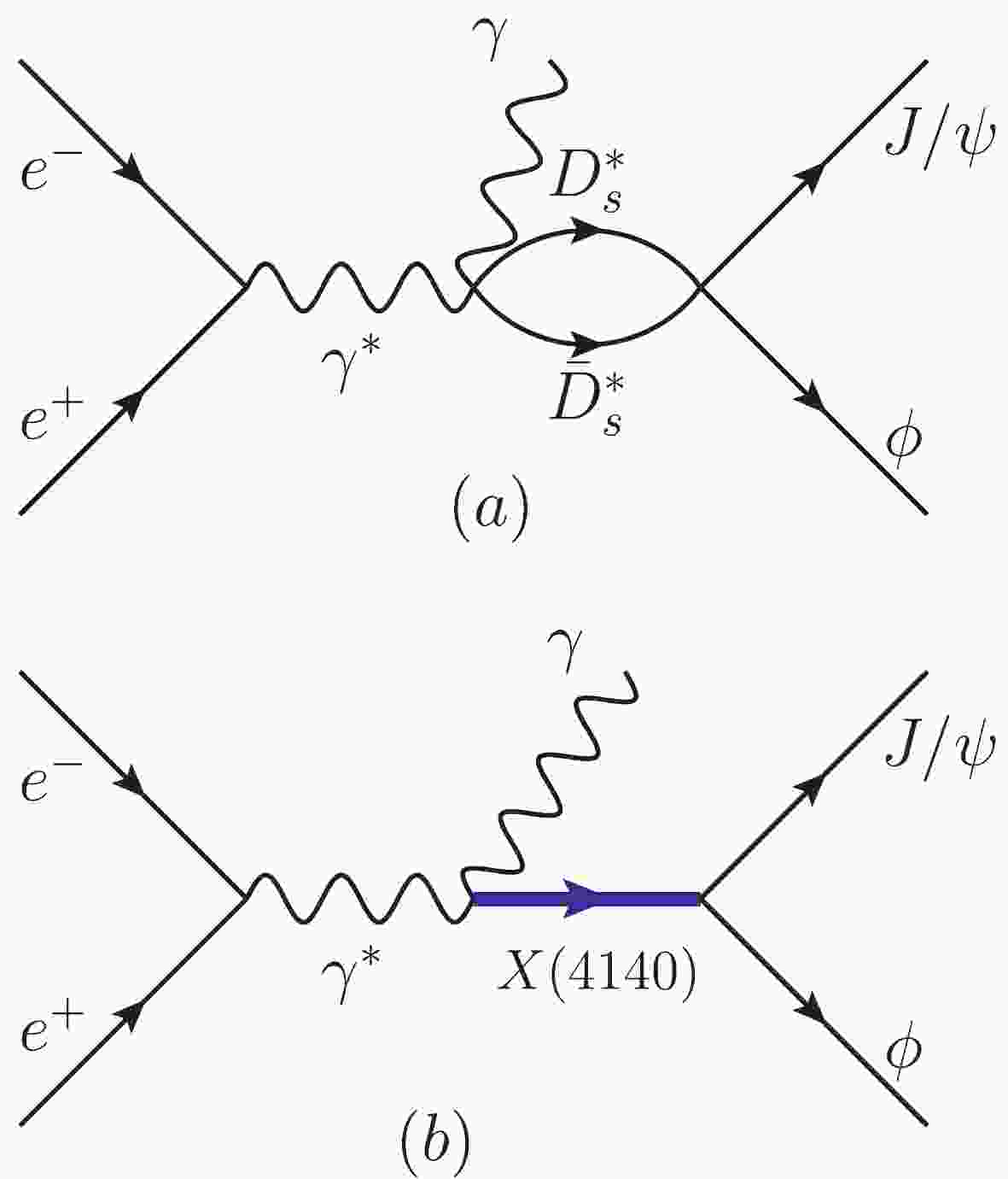
where $ \epsilon_\mu $, $ \epsilon_\alpha $, $ \epsilon_\gamma $, and $ \epsilon_\beta $ are the polarization vectors for the virtual photon $ \gamma^* $, outgoing photon $ \gamma $, $ J/\psi $, and $ \phi $, respectively. The BESIII collaboration measured the process $ e^+e^- \to \gamma \phi J/\psi $ at $ \sqrt{s} = 4.6 $ GeV, which determines the energy of the virtual photon. The Feynman diagrams for the process are depicted in Fig. 1. This reaction can proceed through the $ D^*_s\bar{D}^*_s $ interaction, which dynamically generates the $ X(4160) $ resonance, as depicted in Fig. 1(a), and also through the intermediate $ X(4140) $ resonance of Fig. 1(b). Obviously, in the neighborhood of the $ X(4140) $ and $ X(4160) $ resonances, the tree level term, proportional to the phase space, is small compared to the resonance terms, and therefore we neglect its contribution.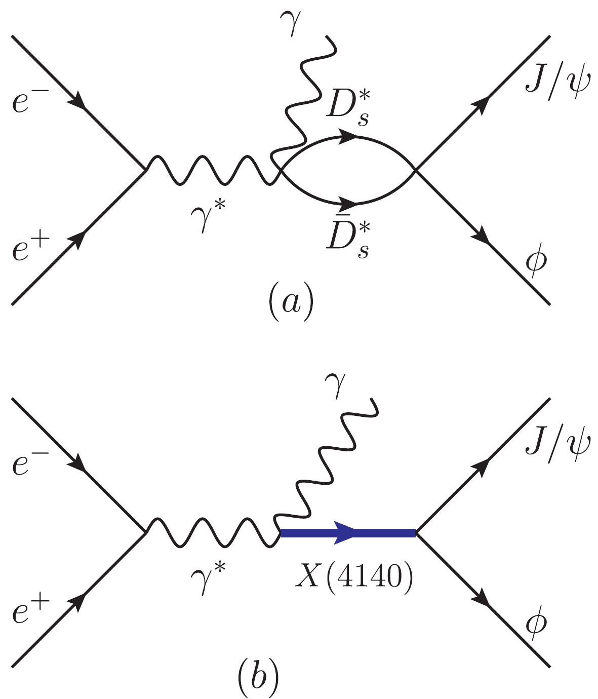

Figure 1.  (color online) Feynman diagrams for the $e^+e^- \to \gamma J/\psi\phi$ process. (a) the contribution of the $D^*_s\bar{D}^*_s$ molecular state $X(4160)$ contained in the $D^*_s \bar{D}^*_s \to J/\psi\phi$ vertex, (b) the contribution of the $X(4140)$ resonance.

Let us look at the amplitude of the process depicted in Fig. 1(a). We have,

where $ A' $ is an unknown constant for the vertex $ \gamma\gamma^*\to D_s^*\bar{D}_s^* $, P ($ \equiv \sqrt{s} $) is the $ e^+e^- $ total momentum, $ t_{D_s^*\bar{D}_s^*,\phi J/\psi} $ is the transition matrix element from $ D_s^*\bar{D}_s^* $ to $ \phi J/\psi $, which is evaluated with coupled channels in Ref. [6] and contains the resonant structure of the state, and q is the momentum of $ D^*_s $. $ {\cal{D}}(q) $ is the vector meson propagator, without the $ (-g_{\rho\rho'}+q_\rho q_{\rho'}/M_{D^*_s}^2) $ term, which comes from the sum over polarizations $ \epsilon_\rho \epsilon_{\rho'} $, and $ t^\mu_{e^+e^-} $ is the $ e^+e^-\gamma^* $ vertex given in Ref. [16],

with $ u_{r'} $ ($ p_2 $), $ v_r $ ($ p_1 $) the four spinors (momenta) of $ e^- $ and $ e^+ $, respectively. We immediately find for the average over $ e^+e^- $ polarizations,

and neglecting the electron mass $ m_e $,

The $ {\rm i} \int \displaystyle\frac{{\rm d}^4q}{(2\pi)^4}{\cal{D}}{\cal{D}} $ term in Eq. (2) gives rise to the loop function $ G_{D^*_s\bar{D}^*_s} $, which is a function of $ M_{\rm inv}(\phi J/\psi) $. Since we know the $ D_s^*\bar{D}_s^* \to \phi J/\psi $ transition amplitude and loop function in the $ \phi J/\psi $ rest frame, we shall work in that frame in what follows. In Eq. (2), we have written the generic polarization vectors for the external particles $ \gamma $, $ \phi $, $ J/\psi $. Next, we look at the spin structure. Since the resonance $ X(4160) $ is $ 2^{++} $ coming from the vector in s-wave, the generic polarization vector for $ D_s^*\bar{D}_s^* \to \phi J/\psi $ becomes,

where the indices $ \beta $, $ \gamma $, m and $ m' $ are now spatial $ (1,2,3) $, since we are neglecting the $ \epsilon^0 $ component of these vectors. This can be done because the three momenta of these vectors are much smaller than their masses. A detailed evaluation of the accuracy of this approximation is done in Ref. [17] (see Appendix A of that work), with the conclusion that, for a problem like the present one, the error omitting $ \epsilon^0 $ is of the order of 1%. This approximation can be extended to the vector polarizations in the $ D_s^*\bar{D}_s^* $ propagator, since $ {\rm d}^3 \vec{q} $ is restricted to momenta $ |\vec{q}\; |<q_{\rm max} $, with $ q_{\rm max} \simeq 600 \sim 700 $ MeV. Furthermore, most of the contribution to the integral comes from momenta lower than $ q_{\rm max} $ [18-20].

For the $ D^*_s $ propagator, we can now write the structure of the polarization vectors,

and as a consequence, the tensor structure $ \epsilon_{\beta}\epsilon_{\gamma} $ of Eq. (6) is translated to $ \epsilon_\rho \epsilon_\sigma $ of Eq. (2) that couples to $ \gamma $ $ \gamma^* $. For $ \gamma $ and $ \gamma^* $, we can also have the s-wave and this forces the structure,

where $ \beta $, $ \gamma $, n are also spatial indices.

The $ \gamma^* $ propagator in Eq. (2), after summing over polarizations (virtual photon), gives,

with spatial indices $ \beta $, $ \gamma $.

In principle, conserving the total spin and parity, we can also have $ L = 2 $ and spin zero, which corresponds to a structure,

where $ \vec{p} $ is the $ \gamma $ momentum in the rest frame of the system $ \phi J/\psi $ ,

with $ \lambda(x,y,z) = x^2+y^2+z^2-2xy-2yz-2xz $. To compare with the former structure, we must make the amplitude of Eq. (10) dimensionless, which means that $ \vec{p} \to \vec{p}/M_{J/\psi} $, or $ \vec{p}/M_{D^*_s} $, or $ \vec{p}/M_\phi $. In either case, the contribution of this term to $ |{{\cal{M}}}^{(a)}_{J/\psi \phi}|^2 $ is very small ($ \sim 10^{-2}- 10^{-4} $) and can be neglected. This conclusion leads to the general rule that reactions proceed with the smallest possible value of L. This is a consequence of the factor $ \vec{p}^{\,2} $ that introduces a $ M_{\rm inv}(\phi J/\psi) $ dependence in Eq. (11), apart from the one we shall discuss next, but is in any case smooth and does not distort the resonant shapes induced by the resonances.

With the above conclusion, the amplitude of Eq. (2) takes the form,

which by symmetry can be simplified to,

with,

and,

where the sum over repeated indices is implied. We sum next over the polarizations of $ \phi $, $ J/\psi $, but not $ \gamma $, and the indices j, $ j' $. One can do the explicit exercise, but it is unnecessary because the only indices that remain are l and s, and the only polarization vectors left are the two $ \epsilon(\gamma) $. There can be only two possible combinations,

and

so that we have,

where the external $ \gamma $ momentum $ \vec{p} $ in the rest frame of the $ \phi J/\psi $ system is given by Eq. (11), and we have taken explicitly into account the two transverse polarizations of the external photon.

Thus finally,

with $ \delta_{ls}-\displaystyle\frac{p_l p_s}{\vec{p}^{\,2}} $ replaced by $ 2\delta_{ls} $ in the second case of Eq. (20). The contribution of the two parentheses of Eq. (21) gives,

or for the case of $ 2\delta_{ls} $,

As mentioned, the calculations are done in the $ \phi J/\psi $ reference frame, hence, $ p_1 $, $ p_2 $, $ E_1 $, $ E_2 $ in the former equations are evaluated in that frame. It is easy to relate them with the momenta $ p'_1 $, $ p'_2 $ of $ e^+ $, $ e^- $ in the $ e^+e^- $ rest frame. Indeed, to pass from this frame to the $ \phi J/\psi $ rest frame, we use the velocity of $ \phi J/\psi $ in the $ e^+e^- $ frame,

with

For the average of $ M(\phi J/\psi) $ in the range of our study, we find $ |\vec{v}|\simeq 0.09 $. This is a non-relativistic velocity in the sense that $ \vec{v}^{\,2} $ can be neglected, and $ \sqrt{1-\vec{v}^{\,2}} \simeq 1 $. Actually we find,

Coming back to Eq. (22), we find,

which, neglecting $ m^2_e $ and $ v^2 $, becomes,

where $ \theta $ is the angle between $ \vec{p}^{\,\prime}_1 $ and $ \vec{p} $. After the phase space integration, $ {\rm cos}^2\theta $ becomes $ 1/3 $. What matters from this result is that since,

and the square of the photon propagator $ 1/{P^4} $ in Eq. (21) is $ 1/{s^2} $, $ |{\cal{M}}^{(a)}_{J/\psi \phi}|^2 $ from Eq. (16) goes as $ 1/s $ and the only $ M_{\rm inv}(\phi J/\psi) $ dependence comes exclusively from $ |\tilde{{\cal{M}}}^{(a)}_{J/\psi\phi}|^2 $. For the term $ 6E_1E_2-2 \vec{p}_1\cdot\vec{p}_2 $ in Eq. (23) we find the same result, and neglecting $ m^2_e $ and $ \vec{v}^{\,2} $ it becomes $ 6 \left( \vec{p}^{\,\prime}_1 \right)^2 +2\left( \vec{p}^{\,\prime}_1 \right)^2 $, independent of $ M_{\rm inv}(\phi J/\psi) $.

In Ref. [6], dimensional regularization was used for the G loop function appearing in Eq. (12). It was pointed out in Ref. [21] that the G function in the charm sector can eventually become positive below the threshold and give rise to the pole $ (V^{-1}-G) $ with a repulsive potential, which is physically unacceptable. This is not the case in Ref. [6]. Here, we use the cut-off method with a fixed $ q_{\rm max} = 630 $ MeV such that it gives the same value at the pole position as G with the dimensional regularization used in Ref. [6]. We also use the dimensional regularization form to evaluate uncertainties in the formalism.

With the couplings of $ X(4160)(\equiv X_1) $ to $ D^*_s\bar{D}^*_s $ and $ J/\psi\phi $ obtained in Ref. [6], the amplitude for the $ D^*_s\bar{D}^*_s \to J/\psi \phi $ transition has the following form,

where $ g_{D^*_s\bar{D}^*_s} = (18927-5524{\rm i}) $ MeV and $ g_{J/\psi \phi} = (-2617- $$5151{\rm i}) $ MeV, $ M_{X_1} = 4160 $ MeV [6], and,

where $ \Gamma_0 $ accounts for the channels of Ref. [6] not explicitly considered here, and,

where $ \tilde{p}_\phi $ and $ \tilde{p}_{D^*_s} $ are the $ \phi $ and $ D^*_s $ momenta in the rest frame of $ J/\psi\phi $ and $ D^*_s\bar{D}^*_s $, respectively,

Let us mention in passing that the couplings in Eq. (32), as obtained in Ref. [6], are complex. This is a consequence of the use of a unitary scheme in the coupled channels, but not in the individual channels. This is common to all unitary coupled channel studies [6,18-20,22-26]. Hence, it should not be surprising that individual diagonal amplitudes are not unitary. Nevertheless, note that in the non-diagonal amplitude of Eq. (32), the imaginary parts are small and their role in $ |{\cal{M}}^{(a)}_{J/\psi \phi}|^2 $ is basically negligible.

Let us now discuss the role of the other resonance. $ J/\psi\phi $ can also be produced via the $ X(4140) $ ($ 1^{++} $) resonance, as depicted in Fig. 1(b). Taking suitable operators for the vertex of $ X(4140) $ [$ \equiv X_2 $] to $ \gamma^*\gamma $

and to $ J/\psi\phi $,

we get

with

Thus, the amplitude for the diagram in Fig. 1(b), up to the $ t^\mu_{e^+e^-} $ and $ \gamma^* $ propagator of Eq. (2), can be written as,

where $ M_{X_2} = 4135 $ MeV and $ \Gamma_{X_2} = 19 $ MeV, the same as those of Ref. [4], and $ B' $ corresponds to the strength of the contribution of the $ X(4140) $ resonance term.

We can now proceed as in the former case and show also that after the boost, $ \sum_{\rm pol} t^\mu_{e^+e^-} t^{\nu*}_{e^+e^-} $ of Eq. (5) only depends on s and not on $ M_{\rm inv}(\phi J/\psi) $. In this case, one could have a p-wave coupling to $ \gamma^*\gamma $, which introduces a factor p in the $ {{\cal{M}}}_{J/\psi\phi}^{(b)} $ amplitude that depends smoothly on $ M_{\rm inv}(\phi J/\psi) $. For the same reasons as before, this term should be very small and we neglect it. Also, since the $ X(4140) $ resonance is very narrow, the change of p in the range of the resonance is very small and its effect in the $ M_{\rm inv}(\phi J/\psi) $ dependence would anyway be negligible.

Another relevant aspect for the present work is that the two structures $ \tilde{{\cal{P}}}^{(a)}_{l,j}(\phi J/\psi) $ and $ {\cal{P}}^{(b)} $ do not interfere when one sums over polarizations of all final states, since $ \epsilon(\phi) \times \epsilon(J/\psi) $ is antisymmetric in the vectors, while $ \tilde{{\cal{P}}}^{(a)}_{l,j} $ of Eq. (15) is symmetric.

Finally, the $ J/\psi\phi $ invariant mass distribution in the process $ e^+e^- \to \gamma J/\psi \phi $ can be written as,

where $ \tilde{p}_\phi $ is given in Eq. (36), and $ k' $ is the momentum of the outgoing photon in the c.m. frame of $ e^+e^- $,

and,

where we incorporate in A and B the factors $ A' $ and $ B' $, the terms from the $ e^+e^- $ vertex and photon propagator, the factors from the sum over vector polarizations, and the factors of the formula for the cross-section of $ e^+e^- $, all of which are independent of $ M_{\rm inv}(\phi J/\psi) $.

It should be pointed out that we neglect the mechanism for $ J/\psi\phi $ produced primarily from the virtual photon decay, with the $ J/\psi\phi $ intermediate state instead of $ D^*_s\bar{D}^*_s $ in Fig. 1(a), which would involve an extra factor $ g_{J/\psi\phi}/g_{D^*_s\bar{D}^*_s} $ in the amplitude of Fig. 1(a). We expect that it provides a small contribution compared with that of Fig. 1(a).

As the $ X(4160) $ state mainly couples to the $ D^*_s\bar{D}^*_s $ channel according to Ref. [6], it is interesting to predict the $ D^*_s\bar{D}^*_s $ mass distribution in the process $ e^+e^-\to \gamma D^*_s\bar{D}^*_s $, which can be used to test the relevance of the $ X(4160) $ resonance.

The mechanism of this process is depicted in Fig. 2. In addition to the contribution of the $ D^*_s\bar{D}^*_s $ molecular state $ X(4160) $, as shown in Fig. 2(b), we also take into account the tree level term of Fig. 2(a), which is small compared to the $ D^*_s\bar{D}^*_s $ interaction term in the region around the $ X(4160) $ resonance. Since the threshold of $ D^*_s\bar{D}^*_s $ is about 60 MeV higher than the $ X(4160) $ mass, we will keep the tree level term in our calculation.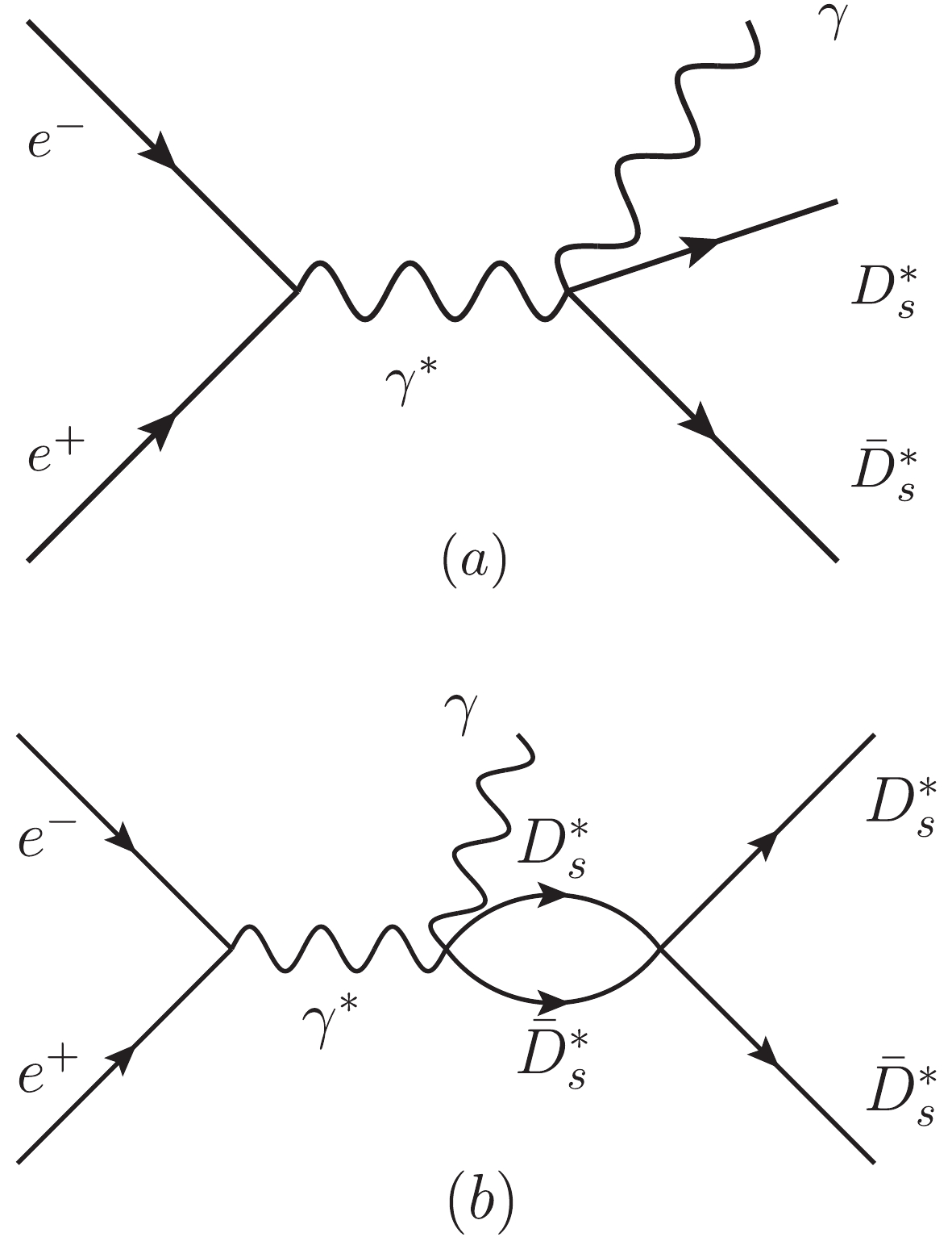

Figure 2.  Feynman diagrams for the $e^+ e^-\to \gamma D_s^*\bar{D}_s^*$ process. (a) the tree level term, (b) the contribution of the $D^*_s\bar{D}^*_s$ molecular state $X(4160)$.

In analogy to the process $ e^+e^- \to \gamma J/\psi \phi $, the $ D^*_s\bar{D}^*_s $ mass distribution in the process $ e^+e^-\to \gamma D^*_s\bar{D}^*_s $ can be written as,

with $ k' $ given by Eq. (44) with $ M_{\rm inv}(J/\psi \phi) $ substituted by $ M_{\rm inv}(D^*_s\bar{D}^*_s) $, and,

where the factor A and the loop function G are the same as those of Eq. (45). The transition amplitude $ t_{D^*_s\bar{D}^*_s,D^*_s\bar{D}^*_s} $ is given in terms of the coupling $ g_{D^*_s\bar{D}^*_s} $ obtained in Ref. [6] ,

We would like to make an observation concerning the gauge invariance of the model. We recall that we have taken spin structures consistent with having the process proceeding in s-wave, with the implicit assumption that the lowest partial wave amplitudes give the largest contribution to the process. We even estimated that the effects of higher partial waves are very small. As a result, we also simplified the formalism and made it manifestly non-covariant, which makes the nontrivial calculations easier. Given these facts, the test of gauge invariance, which requires the amplitude to vanish under substitution of $ \epsilon_\mu(\gamma) $ by $ p_\mu(\gamma) $, cannot be done. In addition, when taking the lowest angular momentum contribution, while this is a good approximation for the amplitude, one is omitting terms that can be essential for the test of gauge invariance, which means that in such a case the test of gauge invariance would not be satisfied. However, we are relying on a specific gauge, the Coulomb gauge, where photons are transverse and have null time polarization component [see Eq. (19) for the sum over the transverse polarizations]. This situation appears in some physical processes, like the radiative capture of pions by nuclei [27], where one considers only the manifestly non-gauge invariant Kroll-Ruderman term, because the pion pole term required for gauge invariance is null in the Coulomb gauge [28]. The same situation appears when using vector meson dominance to evaluate amplitudes for photon processes, where removing the longitudinal vector components before vector-photon conversion is suggested as a method which is implicitly consistent with gauge invariance [29,30].

As discussed above, there are three free parameters in our model for the process $ e^+e^- \to \gamma J/\psi \phi $: (I) A, an overall normalization factor, (II) B, the strength of the contribution of the $ X(4140) $ resonance term, (III) $ \Gamma_0 $, accounting for the channels of Ref. [6] not explicitly considered in this paper. In our previous work [4], a similar mechanism for $ J/\psi\phi $ production was used to describe the $ J/\psi\phi $ mass distribution in the $ B^+\to J/\psi\phi K^+ $ decay measured by the LHCb collaboration [7, 8], and $ \Gamma_0 $ was extracted as $ 67.0\pm 9.4 $ MeV. We take this value of $ \Gamma_0 $ and fit the other two parameters (A and B) to the BESIII data for the $ J/\psi\phi $ mass distribution in the process $ e^+e^- \to \gamma J/\psi \phi $ from the threshold to 4250 MeV at $ \sqrt{s} = 4.6 $ GeV [10]. The resulting $ \chi^2/d.o.f. \approx 6.1/(12-2) = 0.61 $ is very small, mainly because of large errors in the data. We present the $ J/\psi\phi $ mass distribution in Fig. 3, where we see that there is a significant peak around 4135 MeV, associated with the $ X(4140) $ resonance. This is in agreement with the BESIII measurements, although the BESIII collaboration concluded that there is no structure in the $ J/\psi\phi $ mass distribution because of low statistics. In addition, we also find a broad bump around the mass of the $ X(4160) $ resonance, and a sizeable cusp structure around the $ D^*_s\bar{D}^*_s $ threshold, both resulting from the dynamically generated $ X(4160) $ resonance. This is also compatible with the low statistics measurements of the BESIII collaboration [10].

Figure 3.  (color online) The $J/\psi\phi$ invariant mass distribution in the process $e^+e^- \to \gamma J/\psi \phi$. The magenta dashed line and the blue dotted line show the contributions of the $X(4160)$ [Fig. 1(a)] and X(4140) resonances [Fig. 1(b)], respectively. The red solid line corresponds to the full contribution. The experimental data are from the BESIII measurements [10]. The band reflects the uncertainties in A and B from the fit, and represents the 68% confidence level.

It should be noted that the peak around 4135 MeV, and the cusp structure close to the $ D^*_s\bar{D}^*_s $ threshold, if confirmed by more accurate measurements, should be associated to the $ X(4140) $ and $ X(4160) $ resonances. In Fig. 4, we present our results by increasing $ A^2 $, and find that the broad bump and the cusp become clearer. The cusp comes from the factor $ G_{D^*_s\bar{D}^*_s} $, and reflects the analytical structure of this function with a discontinuity of the derivative at the threshold. The bump and the cusp structure appearing in Fig. 3 are due to the $ D^*_s\bar{D}^*_s $ molecular nature of the $ X(4160) $ resonance. Thus, we strongly suggest that the BESIII collaboration measures this process with better statistics.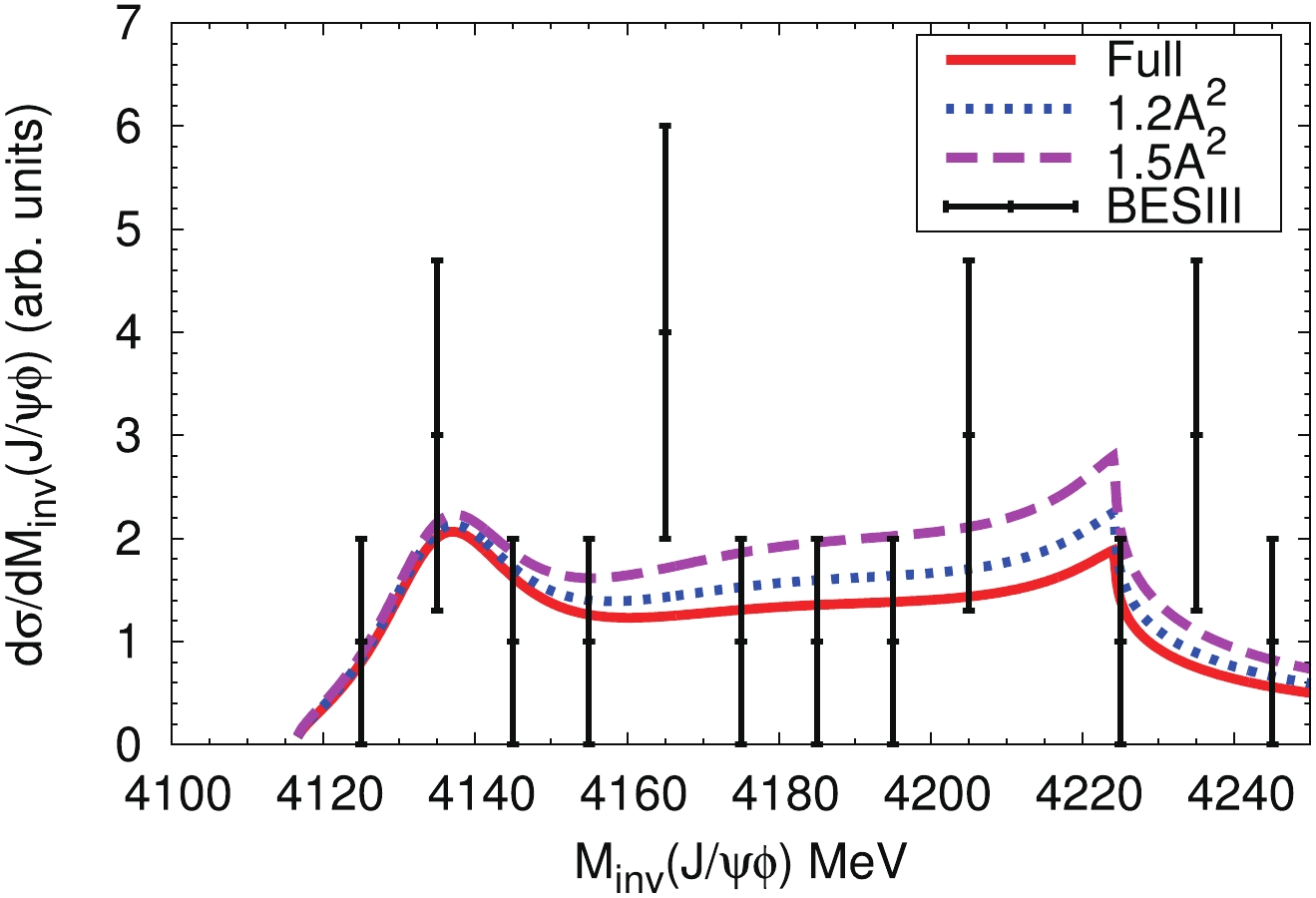

Figure 4.  (color online) The $J/\psi\phi$ invariant mass distribution in the $e^+e^- \to \gamma J/\psi \phi$ process by increasing $ A^2 $ to $ 1.2A^2 $ (magenta dashed line) and $1.5A^2$ (blue dotted line). The other parameters are the same as in Fig. 3.

Before the BESIII measurements [10], the process $ e^+ e^- \to \gamma J/\psi \phi $ was analyzed around the c.m. energy of the thresholds of $ D_{s0}D^*_s $, $ D_{s1}D_s $ and $ D_{s1}D^* $ in Ref. [31], which suggested that the anomalous triangle singularity can provide a resonance-like peak in the $ J/\psi\phi $ invariant mass distribution around the $ D^*_s\bar{D}^*_s $ threshold. Thus, a more accurate measurement of this process can also be useful to distinguish the different interpretations of the structure around the $ D^*_s\bar{D}^*_s $ threshold.

Finally, as a test of the interpretation given here, we also present in Fig. 5 the $ D^*_s\bar{D}^*_s $ invariant mass distribution in $ e^+e^- \to \gamma D^*_s\bar{D}^*_s $ with the same parameters as above. It is seen that there is an enhancement close to the threshold, significantly different from the phase space (labeled as 'tree'). The peak is the reflection of $ X(4160) $ and should not be misidentified as a new resonance. We also stress that the strength of this distribution is predicted relative to Fig. 3 . This distribution could be measured experimentally and hence produce a further test of the ideas presented in this work.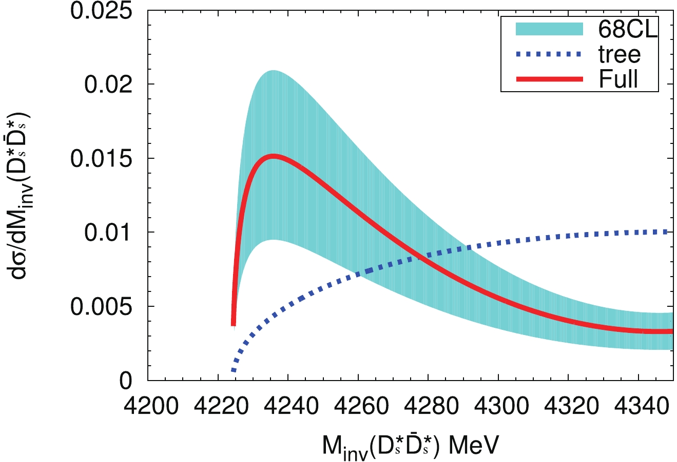

Figure 5.  (color online) The $D^*_s\bar{D}^*_s$ invariant mass distribution in the process $e^+e^- \to \gamma D^*_s\bar{D}^*_s$. The results are normalized to the same area around the $D^*_s\bar{D}^*_s$ threshold at 4350 MeV. The blue dotted line and red solid line correspond to the contributions of the tree level term [Fig. 2(b)], and the full contribution, respectively. The band reflects the uncertainties of parameter B in the fit, and represents the 68% confidence-level.

Equation (32) is valid around the resonance peak but we are extrapolating it to the $ D^*_s\bar{D}^*_s $ threshold. It would be interesting to have the amplitude in the coupled channel unitary approach [6] and see if there are changes which could help estimate the uncertainties. We reproduce the result of Ref. [6] in a simplified way here, using at the same time the dimensional regularization for the G function. The most important channels for the $ X(4160) $ resonance in the range of the $ J/\psi\phi $ invariant masses of the present reaction are the $ D^*_s\bar{D}^*_s $ and the $ J/\psi\phi $ channels. We consider these two channels and take the full strength of the light vector channels in the most important one, the $ \phi\phi $ channel. The purpose is to generate the $ \Gamma_0 $ width of Eq. (33), which is otherwise kept constant in the range of invariant masses considered. In fact, given the large amount of the phase space available for the decay, its relative change in the region of interest is small. The coupled channel method gives rise automatically to $ \Gamma_{J/\psi \phi} $ and $ \Gamma_{D^*_s\bar{D^*_s}} $, and we do not need to evaluate them since the method provides directly the transition matrices $ t_{D^*_s\bar{D^*_s},J/\psi\phi} $, incorporating $ \Gamma_{J/\psi \phi} $ and the Flatté effect produced by $ \Gamma_{D^*_s\bar{D}^*_s} $.

We solve the Bethe-Salpeter equation in coupled channels,

where G is the diagonal matrix diag$ [G_{D^*_s\bar{D}^*_s}, G_{J/\psi\phi}, G_{\phi\phi}] $, and V is the matrix,

where the channels 1, 2, 3 are $ D^*_s\bar{D}^*_s $, $ J/\psi\phi $ and $ \phi\phi $. $ V_{11} $, $ V_{12} $, $ V_{21} $, $ V_{22} $, are taken from Ref. [6], and the magnitude $ a = 110 $ is chosen such that,

where $ \tilde{p}_\phi $ is the $ \phi $ momentum in the $ X(4160)\to \phi\phi $ decay, and $ g_{\phi\phi} $ the coupling at the $ X_1 $ pole of the $ X(4160) $ resonance. The subtraction constants in G are $ \alpha_{D_s^*\bar{D}_s^*} = -2.19 $ and $ \alpha_{J/\psi \phi} = -1.65 $ , respectively for the $ D^*_s\bar{D}^*_s $ and $ J/\psi\phi $, taken from Refs. [6, 32]. Since we are only interested in the $ \Gamma_0 $ width, it is sufficient to take $ i {\rm Im}G_{\phi\phi} $ with,

with $ q_\phi = \lambda^{1/2}(M^2_{\rm inv}, m^2_\phi, m^2_\phi)/2M_{\rm inv} $. This simplified approach to a more enlarged coupled channel problem has proven successful in Ref. [33]. The method provides the G function and the transition amplitudes directly.

In Fig. 6, we show the modulus squared of the transition amplitudes $ |t_{D^*_s\bar{D}^*_s,D^*_s\bar{D}^*_s}|^2 $, $ |t_{D^*_s\bar{D}^*_s,J/\psi\phi}|^2 $, $ |t_{D^*_s\bar{D}^*_s,\phi\phi}|^2 $, given by Eq. (50). As can be seen, the peaks are around 4160 MeV, and two cusp structures are found at the thresholds of $ J/\psi\phi $ and $ D^*_s\bar{D}^*_s $, respectively. With the above formalism, we make again a fit of the data by changing the parameters A and B, with a resulting $ \chi^2/d.o.f. \approx 6.6/(12-$$2) = 0.66 $. We present the $ J/\psi\phi $ mass distribution in Fig. 7, where we find a clear peak around 4135 MeV, and a broad bump around the mass of $ X(4160) $. There is also a cusp structure around the $ D^*_s\bar{D}^*_s $ threshold, which is softer than in Fig. 3. We also present the $ D^*_s\bar{D}^*_s $ mass distribution with the new fit parameters in Fig. 8, where the enhancement of the mass distribution close to the $ D^*_s\bar{D}^*_s $ threshold is not as strong as in Fig. 5, but is clearly different from the phase space distribution (labeled as ‘tree’).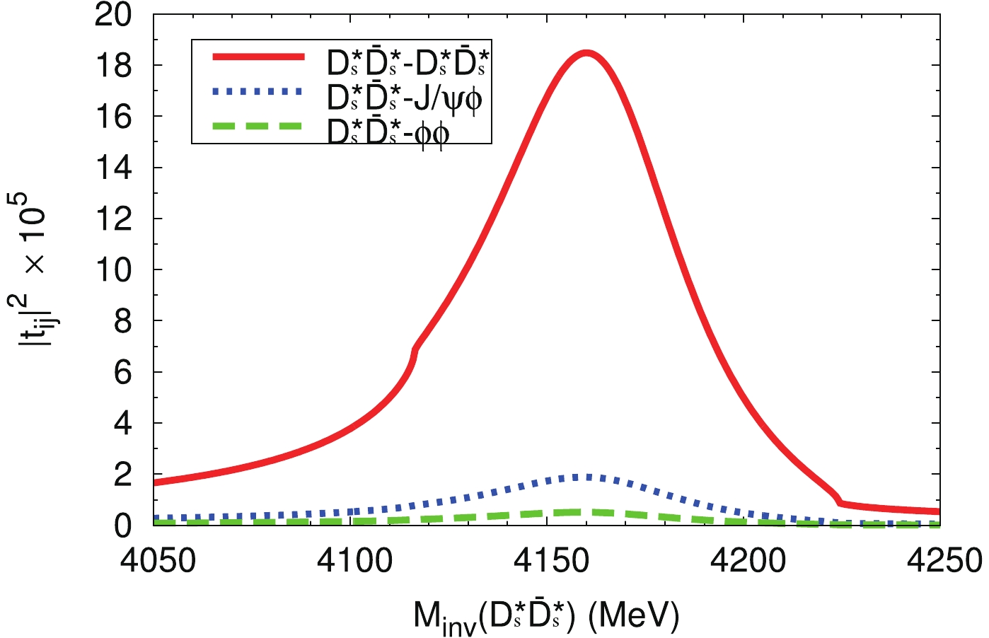

Figure 6.  (colon online) The modulus squared of the transition amplitudes $|t_{D^*_s\bar{D}^*_s,D^*_s\bar{D}^*_s}|^2$, $|t_{D^*_s\bar{D}^*_s,J/\psi\phi}|^2$, $|t_{D^*_s\bar{D}^*_s,\phi\phi}|^2$, given by Eq. (50).

Figure 7.  (color online) The $J/\psi\phi$ invariant mass distribution in the process $e^+e^- \to \gamma J/\psi \phi$ with the new fit parameters. The explanation of the curves is the same as in Fig. 3.

Figure 8.  (color online) The $D^*_s\bar{D}^*_s$ invariant mass distribution in the process $e^+e^- \to \gamma D^*_s\bar{D}^*_s$ with the new fit paramteres. The explanation of the curves is the same as in Fig. 5.

The alternative method serves to show the uncertainties in the theoretical analysis of the data that we have carried out. The method allows for a more realistic extrapolation at high $ J/\psi \phi $ invariant masses. A comparison of Figs. 7 and 3 shows indeed that the differences appear in the region of $ M_{\rm inv}(J/\psi\phi)\sim 4220 $ MeV. We also see differences in the strengths between Figs. 8 and 5, although they are compatible within the estimated errors. Yet, the basic features are the same in both approaches: a peak contribution at low $ J/\psi\phi $ invariant mass coming from a narrow $ X(4140) $ and a broad bump resulting from the $ X(4160) $ resonance, together with a cusp structure around the $ D^*_s\bar{D}^*_s $ threshold with a more uncertain strength. In summary, we show that the data are compatible with the interpretation given for the $ B^+\to J/\psi \phi K^+ $ reaction in Ref. [4], with a narrow $ X(4140) $ and a broad $ X(4160) $ responsible for the $ J/\psi\phi $ invariant mass distribution at low invariant masses. A significant improvement of the data for this reaction is necessary to further test the ideas presented in this work.

In addition, it is interesting to note the different interpretation of the data offered here and in Ref. [10]. In Ref. [10], admitting large errors from the lack of statistics and systematic uncertainties, it was shown that the processes $ e^+ e^-\rightarrow \phi \chi_{c1} (\chi_{c2}) $ followed by $ \chi_{c1} (\chi_{c2} $) decaying into $ J/\psi \gamma $, can account for some fraction of the process $ e^+ e^-\rightarrow \phi J/\psi \gamma $, but there is no clear contribution from $ \gamma X(4140) $. On the other hand, in the present work we showed that the mechanisms discussed, albeit with unknown strength, are also unavoidable. We should note that all these mechanisms have a different spin structure and in principle are distinguishable. The satisfactory interpretation of the $ B^+\rightarrow J/\psi \phi K^+ $ reaction along the lines exposed here makes us believe that it should be responsible also for a good fraction of the $ e^+ e^- \rightarrow \phi J/\psi \gamma $ process. Yet, what is clear is that a much better statistics is needed to make any firm conclusions, and the main purpose of this paper is to encourage the experimental effort in this direction.

Recently, the BESIII collaboration studied the $ J/\psi \phi $ invariant mass distribution in the process $ e^+e^-\to \gamma J/\psi \phi $ at the c.m. energy of $ \sqrt{s} = 4.6 $ GeV, and pointed out that there is no structure because of the low statistics. However, based on our previous work on the decay of $ B^+\to J/\psi\phi K^+ $, we anticipate three bump structures in the $ J/\psi\phi $ invariant mass distributions in the $ e^+e^-\to \gamma J/\psi \phi $ process around 4135 MeV, 4160 MeV, and 4230 MeV. Such features seem to be compatible with, or at least not ruled out by, the low statistics of the BESIII data.

In this work, we analysed the process $ e^+e^-\to \gamma J/\psi \phi $ by considering the contributions of the $ X(4160) $ resonance, as a $ D^*_s\bar{D}^*_s $ molecular state, and of the $ X(4140) $ resonance. Because of the large errors of the BESIII data, the $ \chi^2/d.o.f. $ of the fit is very small. We found a peak around 4135 MeV, associated with the $ X(4140) $ resonance, and a broad bump and a cusp structure, which appear as a consequence of the $ D^*_s\bar{D}^*_s $ molecular structure of the $ X(4160) $ resonance. Thus, we strongly suggest a measurement of this process with higher precision. Finally, as a test of our interpretation, we predicted the $ D^*_s\bar{D}^*_s $ mass distribution in the process $ e^+e^- \to \gamma D^*_s \bar{D}^*_s $ at $ \sqrt{s} = 4.6 $ GeV, and found an enhancement close to the threshold, which is the reflection of the $ X(4160) $ resonance and should not be misidentified as a new resonance.