


 Abstract
 HTML
HTML Reference
 Related
 PDF
PDF


-
Topological charge Q and density
$q\left(x\right)$ are important quantities for investigating the structure of the quantum chromodynamics (QCD) vacuum, and the susceptibility of Q is related to$\eta^{\prime}$ mass by the Witten-Veneziano relation [1, 2]. Lattice QCD is one of the best non-perturbative frameworks for studying QCD properties, in which the space-time is discretized on a lattice.Q on a lattice can be calculated by the gauge field tensor$F_{\mu\nu}$ [3]:$ Q=\int{\rm{d}}^{4}xq\left(x\right)=\frac{1}{32\pi^{2}}\int{\rm{d}}^{4}x{\rm{tr}}\left(\epsilon_{\mu\nu\rho\sigma}F_{\mu\nu}F_{\rho\sigma}\right), $

(1) where the trace is over color indices, and
$\epsilon_{\mu\nu\rho\sigma}$ is a totally antisymmetric tensor. However, the topological charge Q calculated in this way is not always an integer, unlike that in the continuum, unless multiplied by a renormalization factor or calculated on smoothed configurations whose renormalization factor tends to 1. Smoothing methods or other cooling-like methods will change the topological density, and also introduce ambiguous smoothing parameters, like the smoothing time$n_{\rm{sm}}$ , which is always set empirically. Another way to get$q\left(x\right)$ is to evaluate the trace of the chiral Dirac fermion operator in the Dirac and color space [4]:$ q\left(x\right)=\frac{1}{2}{\rm{tr}}\left(\gamma_{5}D_{\rm{chiral}}\right), $

(2) where the trace is over color and Dirac indices,
$\gamma_{5}$ is the Dirac gamma matrix, and$D_{\rm{chiral}}$ is the chiral Dirac fermion operator on a lattice. In this definition, Q will always be an integer due to the Atiyah-Singer index theorem [5], but is hard to calculate exactly as evaluating the trace of$D_{\rm{chiral}}$ is a very computationally costly task. As one of the chiral Dirac fermions, the overlap fermion operator [6, 7] is widely used in the studies of the chiral properties of lattice QCD. The massless overlap Dirac operator$D_{\rm{ov}}$ is constructed from a kernel operator, usually using the Wilson Dirac operator$D_{\rm{W}}$ as the kernel:$ D_{\rm{ov}}=1+\gamma_{5}\epsilon\left(\gamma_{5}D_{\rm{W}}\right), $

(3) where the hopping parameter
$\kappa$ in the kernel$D_{\rm{W}}$ is a free parameter, which is not related to the bare quark mass, and$\kappa\in\left(\kappa_{c}, 0.25\right)$ where$\kappa_{c}$ refers to a critical hopping parameter of the Wilson fermion. We take$\kappa=0.21$ in this work.$\epsilon\left(\gamma_{5}D_{W}\right)$ is the sign function:$\begin{split} \epsilon(\gamma_{5}D_{\rm{W}})=&{\rm{sign}}\left(\gamma_{5}D_{\rm{W}}\right)=\frac{\gamma_{5}D_{\rm{W}}}{\sqrt{D_{\rm{W}}^{\dagger}D_{\rm{W}}}} \\=&\gamma_{5}D_{W}\left(c_{0}+\sum\limits_{i=1}^{\infty}\frac{c_{i}}{D_{\rm{W}}^{\dagger}D_{\rm{W}}+q_{i}}\right), \end{split}$

(4) in which the Zolotarev series expansion [8] is introduced. In our work, the 14th-order Zolotarev expansion was applied [9]. To extract the trace of
$D_{\rm{ov}}$ , we need to calculate the trace of$D_{\rm{W}}^{-2}$ , where$D_{\rm{W}}$ is a large sparse matrix. Its rank is$12N_{L}$ , where$N_{L}$ is the number of lattice sites, empirically in the range of$10^{5}\sim10^{8}$ depending on the lattice size. So, the trace of$D_{\rm{W}}^{-2}$ is too computationally costly to be calculated exactly.Fortunately,
$D_{\rm{ov}}$ is a local operator [10], and there are methods to approximately calculate its trace by making use of this property. The multi-probing method is one of these methods [11, 12] that can be used to estimate the trace of the inverse of a large sparse matrix when the inverse exhibits locality. A. Stathopoulos et al. developed the hierarchical multi-probing method and tested it in lattice QCD Monte Carlo calculations [13]. E. Endress et al. used the multi-probing method to tackle the noise-to-signal problems when calculating all-to-all propagator in lattice QCD [14, 15] by applying the Greedy Multicoloring Algorithm to construct the multi-probing source vectors. Their results have shown the validity and efficiency of the multi-probing method.In this work, we employ the symmetric multi-probing(SMP) method to evaluate the topological charge density by calculating
${\rm{tr}}\left(\gamma_{5}D_{\rm{ov}}\right)$ , and show its efficiency by comparing it to the point source method. We introduce the topological charge density, as well as the trace calculations with point sources and SMP sources, in the next section. Subsequently, the calculation results are presented and discussed. We summarize our work in the last section. -
The overlap Dirac operator
$D_{\rm{ov}}\left(x, y\right)_{\alpha\beta, ab}$ on a lattice$L(n_{x}, n_{y}, n_{t}, n_{z})$ is a large sparse matrix, where$n_{\mu}$ denotes the number of sites in the$\mu$ direction,$\mu=x, y, z, t$ ,$\alpha$ $\beta$ are the Dirac indices and a b are the color indices. The topological charge density$q\left(x\right)$ can be obtained by calculating the trace of the massless overlap Dirac operator:$ \begin{split} q(x) & = \frac{1}{2}{\text{t}}{{\text{r}}_{{\text{d}},{\text{c}}}}\left( {{\gamma _5}{D_{{\text{ov}}}}\left( {x,x} \right)} \right)\\& = \frac{1}{2} \sum\limits_{\alpha ,a} {\langle \psi \left( {x,\alpha ,a} \right)|} {\gamma _5}{D_{{\text{ov}}}}\left| {\psi \left( {x,\alpha ,a} \right)} \right\rangle , \end{split} $

(5) where the trace is over the Dirac and color indices,
$|\psi(x, \alpha, a)\rangle$ is a normalized point source vector which has$N_{L}\times N_{d}\times N_{c}$ components, where the lattice volume is$N_{L}=n_{x}n_{y}n_{z}n_{t}$ ,$ N_{d}=$ $4$ ,$N_{c}=3$ . Only one specific$\left(x, \alpha, a\right)$ component takes a nonzero value in the point source. Substituting Eq. (3) and Eq. (4) into Eq. (5), the most computationally costly step in calculating the trace of$D_{\rm{ov}}$ is to compute the multiplication:$ v_{i}=\frac{c_{i}}{D_{\rm{W}}^{\dagger}D_{\rm{W}}+q_{i}}\left|\psi\left(x, \alpha, a\right)\right\rangle, $

(6) which is equivalent to solving the following linear equation:
$ M_{i}v_{i}=b, $

(7) where
$ M_{i}=\frac{1}{c_{i}}\left(D_{\rm{W}}^{\dagger}D_{\rm{W}}+q_{i}\right), \ b=\left|\psi\left(x, \alpha, a\right)\right\rangle . $

(8) This equation has a high computational cost when solving for a large matrix
$M_{i}$ , and the huge number of point sources corresponding to sites on the whole lattice makes things even worse. The computing time to solve Eq. (7) with the Conjugated Gradient(CG) algorithm for one source is more than$\cal{O}\left(N_{L}\right)$ (considering that$M_{i}$ is a large sparse matrix, and that its conditional number grows as$N_{L}$ ), and there are$12N_{L}$ point sources. Hence, the cost of evaluating$Q=\displaystyle\sum_{x}q\left(x\right)$ by calculating the trace of$D_{\rm{ov}}$ with point sources will be larger than${\cal{O}}\left(N_{L}^{2}\right)$ , which is too high, especially for large$N_{L}$ [16, 17], although this is an exact calculation of the topological charge density on a lattice without any approximations. -
We know from above that calculations of the trace of
$D_{\rm{ov}}$ with point sources is quite a costly task. If we introduce a new source vector$\phi$ by adding two point sources:$ \phi\left(x, y, \alpha, a\right)=\psi\left(x, \alpha, a\right)+\psi\left(y, \alpha, a\right), \ x\neq y, $

(9) then Eq. (5) can be rewritten as:
$ \begin{split} q(x)=&\sum\limits_{\alpha, a}\psi\left(x, \alpha, a\right)\tilde{D}_{\rm{ov}}\phi\left(x, y, \alpha, a\right) \\ & -\sum\limits_{\alpha, a}\psi\left(x, \alpha, a\right)\tilde{D}_{\rm{ov}}\psi\left(y, \alpha, a\right), \end{split} $

(10) where
$\tilde{D}_{\rm{ov}}=\displaystyle\frac{1}{2}\gamma_{5}D_{\rm{ov}}$ , and the second term:$ \sum\limits_{\alpha, a}\psi\left(x, \alpha, a\right)\tilde{D}_{\rm{ov}}\psi\left(y, \alpha, a\right)=\sum\limits_{\alpha, a}\tilde{D}_{\rm{ov}}(x, \alpha, a;y, \alpha, a) $

(11) are space-time off-diagonal elements of
$D_{\rm{ov}}$ . Considering the space-time locality of$D_{\rm{ov}}$ , it has an upper bound [10, 16]:$ \left|D_{\rm{ov}}\left(x, \alpha, a;y, \beta, b\right)\right|\leqslant C\exp\left(-\gamma\left|x-y\right|\right), $

(12) where C and
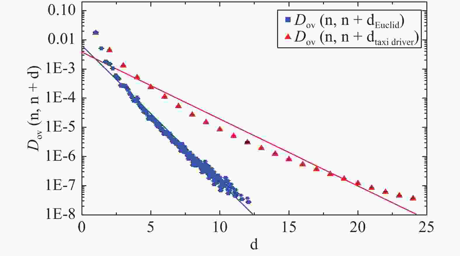
$\gamma$ are constants that do not depend on gauge field configurations, and$\left|x-y\right|$ is defined as the distance between site x and site y. Note that$\gamma_{5}$ only exchanges the elements of$D_{\rm{ov}}$ in the Dirac space, so$\tilde{D}_{\rm{ov}}$ also satisfies this inequality. In the following, ‘off-diagonal’ refers to ‘space-time off-diagonal’ unless otherwise stated. We checked this relation on several lattice configurations, as shown in Fig. 1 .$\gamma$ in the inequality (12) is around$1.076$ from [16] , when$\left|x-y\right|$ is defined as the Euclid distance, and around 0.529 for the taxi driver distance. This result means that the off-diagonal elements of$D_{\rm{ov}}$ are exponentially suppressed as$\left|x-y\right|$ increases, and the inequality (12) holds when the distance is not too small (larger than 3) for the two definitions of distance. We also see that$\gamma$ for the Euclid distance is larger, which means stronger locality, so we adopt this definition in our work.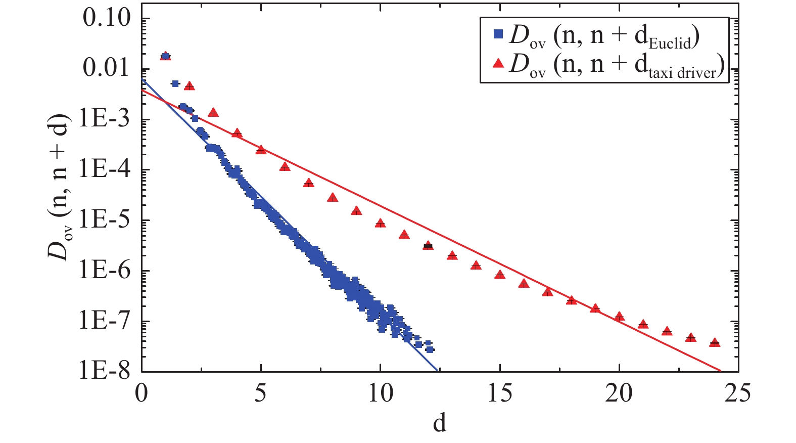
Figure 1. (color online) The locality of
$ {D_{\rm{ov}}}$ is shown by the averaged off-diagonal elements as a function of the Euclid distance and the taxi driver distance, in logarithmic coordinates. The red line is a fit of the taxi driver distance dependence with a slope −0.528, while the blue line is a fit of the Euclid distance dependence with a slope −1.075.The approximate topological charge density
$q\left(x\right)$ can be written as:$ \begin{aligned} q^{\rm{approx}}(x) =&\sum\limits_{\alpha, a}\psi(x, \alpha, a)\tilde{D}_{\rm{ov}}\phi(x, y, \alpha, a), \end{aligned} $

(13) $ \begin{aligned} q^{\rm{approx}}(y) =&\sum\limits_{\alpha, a}\psi(y, \alpha, a)\tilde{D}_{\rm{ov}}\phi(x, y, \alpha, a). \end{aligned} $

(14) We see that the approximate density of both sites can be easily calculated from
$\tilde{D}_{\rm{ov}}\phi(x, y, \alpha, a)$ , and only one linear equation like Eq. (7) needs to be solved to obtain$q\left(x\right)$ and$q\left(y\right)$ , as long as$\left|x-y\right|$ is sufficiently large. This method is called the multi-probing method (MP) or probing method.We first mark all sites in the lattice with a color label, called the coloring algorithm. The sites with the same color form a subset of all lattice sites. The multi-probing source can be constructed from a subset as follows: choose a color and Dirac index, construct point sources on sites in the subset, and add all these point source vectors.
In order to reduce the calculation cost, we would like to reduce the number of MP sources by combining more point sources in one MP source. However, the errors introduced by MP sources depend exponentially on the distance between the sites in the subset, as shown in Eq. (12). To control the systematic errors, we should include in one MP source the sites that as far as possible from each other. Therefore, an appropriate coloring algorithm is important to optimize the balance of the systematic errors and calculation cost.
We chose a symmetric coloring algorithm and the definition of Euclid distance in this work, which marks the sites with the same color in each direction with a fixed distance. There are other algorithms, like GCA (Greedy Coloring Algorithm) [12] , which uses the definition of taxi driver distance. It is convenient to choose the same gap r in all directions, so that the minimal distance of two sites in the subsets is
$r_{\min}=r$ . We call this type of MP source the Normal Mode, and some examples are shown in the left panel of Fig. 2 and Fig. 3.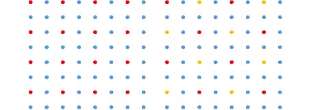
Figure 2. (color online) Example of the Split Mode on a
$ {8\times8}$ 2-D lattice. Red sites in the left panel are colored in the Normal Mode coloring scheme$ {P(4, 4, 0)}$ ; in the right panel, they are split in two subsets with red and yellow colors in the Split Mode scheme$ {P(4, 4, 1)}$ .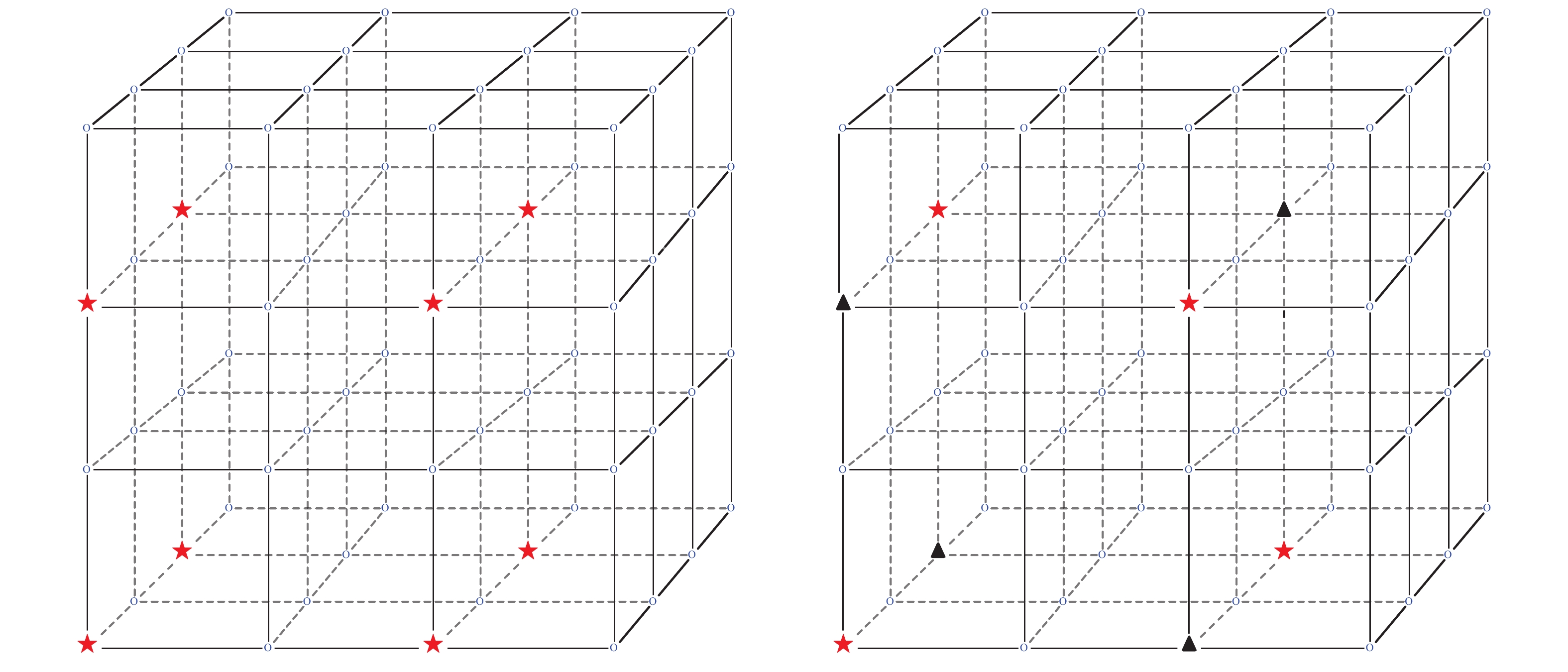
Figure 3. (color online) Examples of the Split Mode on a
${4^3}$ 3-D lattice. Sites denoted with red stars in the left panel are colored in the Normal Mode coloring scheme${P(2, 2, 2, 0)}$ ; in the right panel, they are split in two subsets as red stars and black triangles in the Split Mode scheme${P(2, 2, 2, 1)}$ .Furthermore, we can divided a subset into two subsets by marking half of the sites with a new color, where each site has a different color with respect to its neighbors, see examples in Fig. 2 and Fig. 3 on 2-D and 3-D lattices. In this Split Mode,
$r_{\min}^{\prime}=\sqrt{2}r$ for the two new subsets.We can also combine two subsets into a new subset which includes two sites with equal space-time offsets
$(r/2, r/2, r/2, r/2)$ , where the minimal distance remains unchanged, that is$r_{\min}^{\prime}=r$ for the new subset. We call this mode the Combined Mode, where the number of sites doubles and the errors are increased since more adjoining neighbors are introduced. Note that the Combined Mode only works on 4-D lattices, and r should be even. Fig. 4 and Fig. 5 show examples of the Combined Mode in 2D and 3D situations, where$r_{\min}=r/\sqrt{2}$ and$r_{\min}=\sqrt{3}r/2$ , respectively, after combination.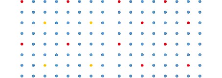
Figure 4. (color online) Example of the Combined Mode on a
${8\times8}$ 2-D lattice. Red sites and yellow sites in the left panel are two subsets colored in the Normal Mode symmetric coloring scheme${P(2, 2, 0)}$ ; in the right panel, they are combined into one with red color in the Combined Mode scheme${P(2, 2, 2)}$ . Note that the minimal distance changes from 4 to${2\sqrt{2}}$ .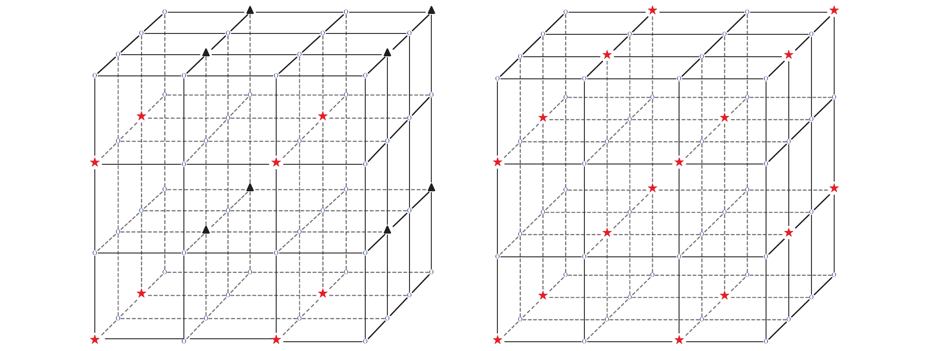
Figure 5. (color online) Example of the Combined Mode on a
${4^3}$ 3-D lattice. Red stars and black triangles in the left panel are two subsets colored in the Normal Mode symmetric coloring scheme${P(2, 2, 2, 0)}$ ; in the right panel, they are combined into one shown by red stars in the Combined Mode scheme${P(2, 2, 2, 2)}$ . Note that the minimal distance changes from 2 to${\sqrt{3}}$ .Let us consider a lattice
$L(n_{x}, n_{y}, n_{z}, n_{t})$ . First, we choose the symmetric coloring scheme$ P\left(m_{x, }m_{y}, m_{z}, m_{t}, {\rm mode}\right) $ , which means that$m_{\mu}$ sites are marked with the same color in the$\mu$ direction of the lattice, and the mode label can be$0, 1, 2$ , which corresponds respectively to the Normal, Split and Combined Mode. We then pick a site$X(x_{1}, x_{1}, x_{3}, x_{4})$ as a seed site, where$x_{\mu}$ denotes its coordinate on the lattice, and we construct an SMP source$\phi_{P}$ in the scheme$P\left(m_{x, }m_{y}, m_{z}, m_{t}, {\rm{mode}}\right)$ :$ \phi_{P}\left(S\left(X, P\right), \alpha, a\right)=\sum\limits_{y\in S\left(X, P\right)}\psi\left(y, \alpha, a\right), $

(15) where
$S\left(X, P\right)$ denotes the site subset that includes all sites with the same color X obtained by the coloring scheme$P\left(m_{x, }m_{y}, m_{z}, m_{t}, {\rm{mode}}\right)$ .The topological charge density on any site
$x\in S\left(X, P\right)$ can be calculated from the combined source:$\begin{split} q^{\rm{approx}}(x)=& \sum\limits_{\alpha, a}\psi(x, \alpha, a)\tilde{D}_{\rm{ov}}\phi_{_{P}}\left(S\left(X, P\right), \alpha, a\right)\\=& q(x)+\sum\limits_{\alpha, a}\sum\limits_{y\in S(X, P)}^{y\ne x}\tilde{D}_{\rm{ov}}(x, \alpha, a;\ y, \alpha, a), \end{split}$

(16) where the second term sums the corresponding off-diagonal components of
$D_{\rm{ov}}$ which satisfy Eq. (12).The lattice sites can be divided into
$N^{\rm{SMP}}$ site sets, with$m_{x}m_{y}m_{z}m_{t}$ sites in each set for${\rm{mode}}=0$ ,$\displaystyle\frac{1}{2}m_{x}m_{y}m_{z}m_{t}$ sites for$\rm{mode}=1$ , and$2\times m_{x}m_{y}m_{z}m_{t}$ sites for$\rm{mode}=2$ . Each site on the lattice should belong to only one set in a specific scheme P. SMP sources are constructed from these symmetric site sets that are only distinct from each other by a few units of coordinate shift. In this case, all SMP sources include the same number of sites for a specific P, which leads to less sources compared with the Greedy Multicoloring Algorithm for the same minimal Euclid distance$\left|x-y\right|$ . Summing Eq. (16) over the lattice volume, the total introduced systematic error for Q is:$ \begin{split} R_{P} =&Q^{\rm{approx}}-Q=\sum\limits_{x\in V}\sum\limits_{\alpha, a}\sum\limits_{y\in S(x, P)}^{y\ne x}\tilde{D}_{\rm{ov}}^{-1}(x, \alpha, a;\ y, \alpha, a) \\& \leqslant6N_{L}C\sum\limits_{y\in S(x, P)}^{y\ne x}\exp\left(-\gamma\left|x-y\right|\right), \end{split} $

(17) where Eq. (12) is used, and the sum over the color and Dirac indices results in a factor of 12. In practice, the errors are far smaller than the upper bound. We define the minimal distance
$r_{\min}^{P}$ for an SMP scheme P, which is the minimal Euclid distance of any two sites in a site set$S\left(X, P\right)$ based on an arbitrary seed site X:$ r_{\min}^{P}=\min\left\{ \left|x-y\right|, \forall x, y\in S\left(X, P\right), \ x\ne y\right\}, $

(18) and we believe that
$\left|x-y\right|=r_{\min}^{P}$ terms will dominate in Eq. (17).For the case of a spatial symmetric lattice
$L\left(n_{s}, n_{s}, n_{s}, \right.$ $\left.n_{t}\right) $ , the SMP scheme can be chosen as$ P\left(\displaystyle\frac{n_{s}}{r}, \displaystyle\frac{n_{s}}{r}, \displaystyle\frac{n_{s}}{r}, \displaystyle\frac{n_{t}}{r}, mode \right) $ so that$ r_{\min}=\begin{cases} r,&{\rm{mode}}=0, 2\\ r\sqrt{2},&{\rm{mode}}=1. \end{cases} $

(19) Therefore, the choice of
$r_{\min}$ should be one of the common factors of$n_{s}$ and$n_{t}$ , or multiplied by$\sqrt{2}$ when$\rm{mode}=1$ , such as$r_{\min}=2$ in the left panel of Fig. 2, and$r_{\min}=2\sqrt{2}$ in the right panel. We choose in this way the appropriate$r_{\min}$ and SMP schemes for different lattices. -
We calculate the topological charge density and the total topological charge for pure gauge lattice configurations with Iwasaki gauge action [18]:
$ S_{\rm{IA}}=\beta c_{1}\left\{ \Omega_{p}+r_{\beta}\Omega_{r}\right\} $

(20) where
$\beta$ is the bare coupling constant,$\Omega_{C}=\displaystyle\sum\frac{1}{3}{\rm{ReTr}}\left(1-\right.$ $ \left.W_{C}\right)$ is the real part of the trace over all Wilson loops$W_{C}$ within a closed contour C, while subscripts p and r refer to a plaquette and$2\times1$ rectangle, respectively.$c_{1}=3.648$ ,$r_{\beta}=-0.09073465$ in Iwasaki action which is an${\cal{O}}\left(a^{2}\right)$ improved gauge field action.First, we calculate the topological charge density exactly with point sources on a
$16{}^{4}$ lattice and compare it to that using SMP sources with$r_{\min}=4\sqrt{2}$ . The results for the topological charge density in the$X-Y$ plane, with$t=1$ and$z=1$ , are shown in Fig. 6. It is obvious that the peaks and valleys are very similar in the results obtained by using point sources and SMP sources, which indicates that the topological structure of the QCD vacuum is well preserved in the SMP method.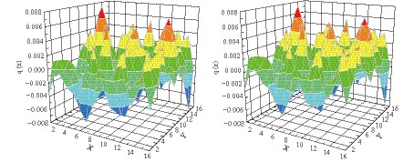
Figure 6. (color online) The topological charge density in the X-Y plane, obtained by plotting
$ {D_{\rm{ov}}}$ with point sources (left), and SMP sources with$ {r_{\min}=4\sqrt{2}}$ (right), in a$ {16^{4}}$ configuration.A series of gauge field configurations were then generated with different lattice spacing a and different lattice volume. The topological charge density for each configuration was evaluated with SMP sources in different schemes, see Table 1, where the SMP scheme P (m, m, m, m, mode) is written as
$\left(m, \rm{mode}\right)$ for short, and the lattice$L\left(n, n, n, n\right)$ is written as$n^{4}$ . The number of point sources$N^{\rm{PT}}$ and SMP sources$N^{\rm{SMP}}$ are presented in Table 2, which are also the number of linear equations, Eq. (7) , that we have to solve by the CG algorithm. It is shown that the cost of calculating the topological charge density sharply reduces for smaller$r_{\min}$ and larger lattices.lattice ${a/}$ fm

No. of config. SMP scheme ${r_{\min}}$ 

${12^{4}}$ 

0.1 20 ${\left(6, 0\right)\;\left(6, 1\right)\;\left(4, 0\right)\;\left(4, 1\right)\;\left(3, 2\right)\;\left(3, 0\right)\;\left(2, 0\right)}$ 

2, ${2\sqrt{2}}$ , 3,

${3\sqrt{2}}$ , 4, 4, 6

0.133 20 ${16^{4}}$ 

0.1 20 ${\left(8, 0\right)\;\left(8, 1\right)\;\left(4, 2\right)\;\left(4, 0\right)\;\left(4, 1\right)\;\left(2, 0\right)}$ 

2, ${2\sqrt{2}}$ , 4, 4,

${4\sqrt{2}}$ , 8

${24^{4}}$ 

0.1 20 ${\left(12, 0\right)\;\left(12, 1\right)\;\left(8, 0\right)\;\left(8, 1\right)\;\left(6, 2\right)\;\left(6, 0\right)}$ 

2, ${2\sqrt{2}}$ , 3,

${3\sqrt{2}}$ , 4, 4

${32^{4}}$ 

0.1 20 ${\left(16, 0\right)\;\left(16, 1\right)\;\left(8, 2\right)\;\left(8, 0\right)}$ 

2, ${2\sqrt{2}}$ , 4, 4

Table 1. Lattice setup and the multi-probing scheme. Symmetric schemes
${P\left(m, m, m, m, \rm{mode}\right)}$ are written as${\left(m, \rm{mode}\right)}$ for short.lattice ${N^{\rm{SMP}}}$ 

${N^{\rm{SMP}}/N^{\rm{PT}}}$ 

${12^{4}}$ 

192, 384, 972, 1944, 1536, 3072, 15552 ${\frac{1}{{1296}},\frac{1}{{648}},\frac{1}{{256}},\frac{1}{{128}},\frac{1}{{162}},\frac{1}{{81}},\frac{1}{{16}}}$ 

${16^{4}}$ 

192, 384, 1536, 3072, 6144, 49152 ${\frac{1}{{4096}},\frac{1}{{2048}},\frac{1}{{512}},\frac{1}{{256}},\frac{1}{{128}},\frac{1}{{16}}}$ 

${24^{4}}$ 

192, 384, 972, 1944, 1536, 3072 ${\frac{1}{{20736}},\frac{1}{{10368}},\frac{1}{{4096}},\frac{1}{{2048}},\frac{1}{{2592}},\frac{1}{{1296}}}$ 

${32^{4}}$ 

192, 384, 1536, 3072 ${\frac{1}{{65536}},\frac{1}{{32768}},\frac{1}{{8192}},\frac{1}{{4096}}}$ 

Table 2. The number of sources
${N^{\rm{SMP}}}$ required in different SMP schemes, and their ratio to the number of point sources${N^{\rm{PT}}}$ .Since
$Q_{P}$ (the topological charge calculated in scheme P) should approach an integer, and the deviation of$Q_{P}$ to its exact value is always smaller than 0.1 as long as$r_{\min}$ is large enough, we extracted the topological charge Q and the absolute value of the systematic error$\left|Q_{P}-Q\right|$ from the series of results with different$r_{\min}$ for each configuration. An example is shown in Fig. 7. The average errors are shown in Fig. 8, and decrease sharply as$r_{\min}$ increases. In general, the average absolute value of the systematic error of$Q_{P}$ and its variance become small enough when$r_{\min}\geqslant4$ . One may note that the error with$r_{\min}=$ $3\sqrt{2} $ on a$24^{4}$ lattice is larger than for$r_{\min}=4$ , which may come from a larger number of nearest neighbor terms (satisfying$\left|x-y\right|=r_{\min}$ in Eq. (17)) for$\rm{mode}=1$ than for$\rm{mode}=0$ . There are 24 nearest neighbors for each site in the former mode, and only 8 nearest neighbors in the latter mode.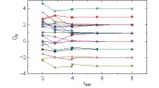
Figure 7. (color online) The series of
${Q_{P}}$ with different${r_{\min}}$ for each configuration on a${16^{4}}$ lattice with${a=0.1}$ fm. When${r_{\min}\geqslant4}$ ,${Q_{P}}$ is very close to an integer. The exact integer numbers of the topological charge can be extracted since the systematic errors are sharply suppressed as${r_{\min}}$ increases.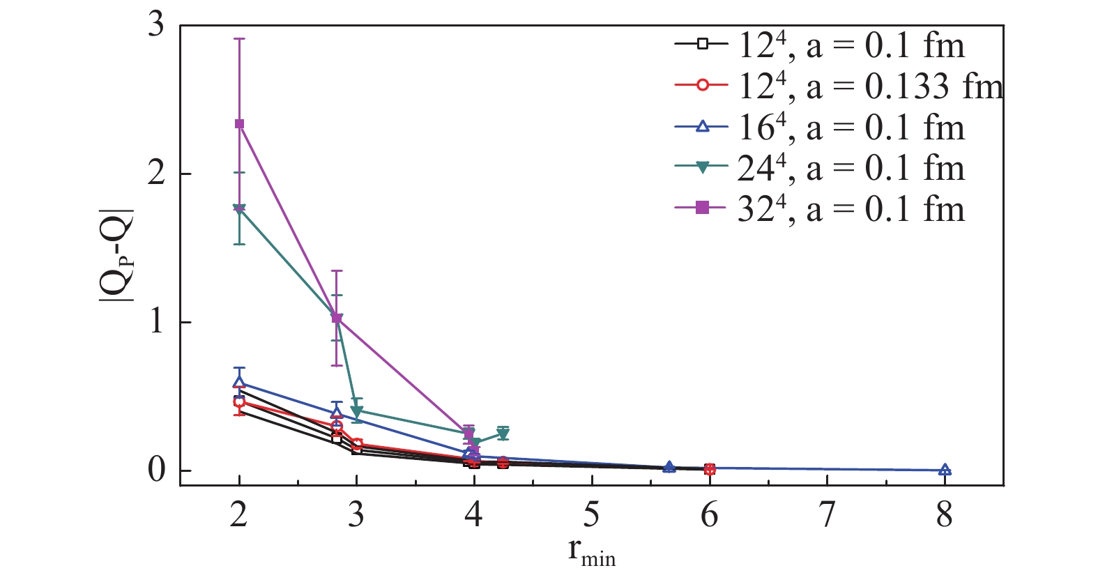
Figure 8. (color online) The average absolute error of QP vs.
${r_{\min}}$ for all lattice settings. For${r_{\min}\geqslant4}$ , the errors are small.Considering the same lattice with different lattice spacing a, Fig. 9 shows that finer lattice spacing a leads to smaller errors. This can also be concluded from Fig. 10, which compares two lattices with the same physical volume. We finally present the errors versus efficiency in Fig. 11, which shows that for larger lattices the calculation of the trace using the SMP method is more efficient for achieving sufficient accuracy.
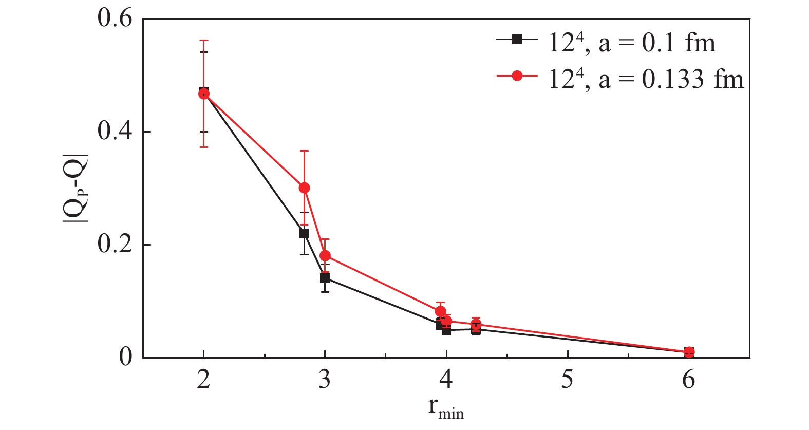
Figure 9. (color online) Comparison of the average absolute error of
${Q_{P}}$ vs.${r_{\min}}$ on a${12^{4}}$ lattice with different a. For the same${r_{\min}}$ , the finer lattice with a smaller a leads to a smaller deviation of QP to an integer.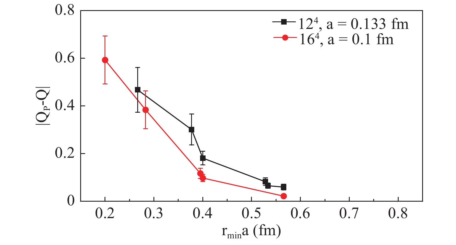
Figure 10. (color online) Comparison of the average absolute error of
${Q_{P}}$ vs. physical distance${r_{\min}a}$ on${V=\left(1.6\;{\rm{fm}}\right)^{4}}$ lattice for different a. In physical units, the errors are also smaller on a finer lattice with the same volume.
Figure 11. (color online) The errors versus the efficiency for all lattices. A larger lattice has a higher efficiency.
All results of
$\left\langle \left|Q_{P}-Q\right|\right\rangle$ are presented in Table 3. We can see, for example, that for$N^{\rm{SMP}}=3072$ , the systematic error increases slowly as the lattice becomes larger. This can be explained by the fact that the number of non-zero off-diagonal elements for SMP sources is proportional to$N_L$ , while$N^{\rm{SMP}}=3072$ is fixed. Therefore, we can expect to apply this method with success on a larger lattice with fixed$N^{\rm{SMP}}$ , where$N^{\rm{PT}}$ is proportional to the lattice volume$N_L$ .L a/fm P NSMP $ {\langle|Q_{P}-Q|\rangle} $ 

L a/fm P NSMP ${\langle|Q_{P}-Q|\rangle} $ 

124 0.1 (6, 0) 192 0.471(71) 164 0.1 (8, 1) 384 0.384(79) (6, 1) 384 0.220(37) (4, 2) 1536 0.0117(21) (4, 0) 972 0.141(24) (4, 0) 3072 0.098(15) (4, 1) 1944 0.051(10) (4, 1) 6144 0.022(3) (3, 2) 1536 0.060(10) (2, 0) 49152 0.003(1) (3, 0) 3072 0.049(7) 244 0.1 (12, 0) 192 1.767(244) (2, 0) 15552 0.010(2) (12, 1) 384 1.029(153) 0.133 (6, 0) 192 0.467(94) (8, 0) 972 0.406(81) (6, 1) 384 0.301(65) (8, 1) 1944 0.253(41) (4, 0) 972 0.181(29) (6, 2) 1536 0.250(36) (4, 1) 1944 0.059(12) (6, 0) 3072 0.186(27) (3, 2) 1536 0.082(16) 324 0.1 (16, 0) 192 2.335(576) (3, 0) 3072 0.065(11) (16, 1) 384 1.026(320) (2, 0) 15552 0.010(2) (8, 2) 1536 0.242(63) 164 0.1 (8, 0) 192 0.592(101) (8, 0) 3072 0.133(29) Table 3. The average absolute systematic error
${\left\langle \left|Q_{P}-Q\right|\right\rangle}$ for different SMP schemes P.There is another method to obtain the topological charge by calculating a few low modes of the chiral Dirac operator, counting the number of zero modes and applying the index theorem. However, to estimate the topological charge density
$q\left(x\right)$ one must calculate more low modes by applying low mode expansion [19]. We compared the calculation cost for the SMP method with the cost of low modes for the overlap operator on$12^{4}$ lattices. We considered$N^{\rm{SMP}}=3072$ with the scheme$P\left(3, 3, 3, 3,\right.$ $ \left. 0\right)$ ,$r_{\min}=4$ in the SMP method, and calculated the low modes of the overlap operator by the Arnoldi algorithm with the number of low modes$N^{\rm{mode}}=100, \ 200$ . The results showed that when$N^{\rm{mode}}=100$ , low mode calculation costs about 18% less than the SMP method, while for$N^{\rm{mode}}=200$ it costs 28% more than the SMP method. However, since the number of zero modes is always an integer, the systematic errors for$q\left(x\right)$ in the low mode expansion could hardly be estimated, while in the SMP method the systematic errors of Q and$q\left(x\right)$ are related. The comparison of$q\left(x\right)$ from the SMP method and the low mode expansion will be an interesting topic for our further studies. -
The topological charge Q and density
$q\left(x\right)$ were calculated from the trace of the overlap Dirac operator employing symmetric multi-probing sources on pure gauge configurations. The systematic errors are reduced as$r_{\min}$ is increased, as expected, due to the locality of the overlap Dirac operator. Thus, the estimated topological charge was close enough to an integer for$r_{\min}\geqslant4$ or$r_{\min}\geqslant4\sqrt{2}$ , in which case the number of required sources was$N^{\rm{SMP}}=12r_{\min}^{4}\ $ $ {\rm{or}}\ 24r_{\min}^{4}$ , as compared to the number of point sources$N^{\rm{PT}}=12N_{L}$ . Note that$N^{\rm{SMP}}$ only depends on the chosen$r_{\min}$ and is independent of$N_{L}$ . Furthermore, we found that the systematic errors of the SMP method for the same$r_{\min}$ increase slowly with larger$N_{L}$ , which means that the computational time for estimating the trace is less dependent on the lattice volume$N_{L}$ . Thus, it is much more economical to employ the SMP method on larger lattices. Since the error in calculating the trace comes from the off-diagonal elements of the matrix, we expect better performance of this method by employing the techniques for suppressing the off-diagonal elements of$D_{\rm{ov}}$ , which we leave for our future work . This method is also believed to work well when dealing with an ultra-local matrix such as the Wilson Dirac operator$D_{\rm{W}}$ , as${\rm{Tr}}D_{\rm{W}}^{-1}$ is very important and quite computationally costly to determinate exactly in lattice QCD.We developed a symmetric scheme with 3 modes of the coloring algorithm and evaluated the topological charge with the SMP method. The results of the average absolute systematic error were presented, as well as the efficiency of the SMP method compared to the point source method. Potential applications of the SMP method are expected in calculations of the trace of the inverse of any large sparse matrix with locality.
Evaluating the topological charge density with the symmetric multi-probing method
- Received Date: 2018-12-03
- Available Online: 2019-03-01
Abstract: We evaluate the topological charge density of SU(3) gauge fields on a lattice by calculating the trace of the overlap Dirac matrix employing the symmetric multi-probing (SMP) method in 3 modes. Since the topological charge Q for a given lattice configuration must be an integer number, it is easy to estimate the systematic error (the deviation of Q to the nearest integer). The results demonstrate a high efficiency and accuracy in calculating the trace of the inverse of a large sparse matrix with locality by using the SMP sources when compared to using point sources. We also show the correlation between the errors and probing scheme parameter


 DownLoad: