


 Abstract
 HTML
HTML Reference
 Related
 PDF
PDF


-
CP violation, as one of the three Sakharov conditions [1], is necessary for explaining the matter-antimatter asymmetry in our universe [2]. Its source could have a close relation with Higgs dynamics [3, 4]. Thus the CP properties of the 125 GeV Higgs boson with spin zero are proposed to be probed in various channels at the Large Hadron Collider (LHC) [5-24]. Among them, the golden channel
$ H\to ZZ\to 4\ell $ has been studied extensively and it gives relatively stringent experimental constraints [19, 21, 22, 24]. On the contrary, the$ H\to\gamma\gamma $ process is another golden channel for discovering the Higgs boson and has a relative clean signature, but it suffers from a lack of CP-odd observable constructed from the self-conjugated diphoton kinematic variables. The CP property of the$ H\gamma\gamma $ coupling can also be studied in the$ H\to\gamma^\ast\gamma^\ast\to 4\ell $ process [25-27]. However, it is challenging due to the low conversion rate of the off-shell photon decaying into two leptons. In this paper, we study the CP property of the$ H\gamma\gamma $ coupling using the interference between$ gg\to $ $ H \to \gamma\gamma $ and$ gg\to \gamma\gamma $ .This interference has been studied in many papers [28-35]. Compared to the Breit-Wigner line shape of the Higgs boson signal, the line shape of the interference term can be roughly divided into two parts: one is symmetric around
$ M_H $ , and the other is antisymmetric around$ M_H $ . These two kinds of interference line shapes have different effects. After integrating over a symmetric mass region around$ M_H $ , the symmetric interference line shape could reduce the signal Breit-Wigner cross-section by ~ 2% [34], while the antisymmetric one has no contribution to the total cross-section, but could distort the signal line shape, and shift the resonance mass peak by$ \sim150 $ MeV [30, 33]. Besides, a variable$ A_i $ is proposed [36, 37] to quantify the interference effect in a sophisticated way, which defines a sign-reversed integral around$ M_H $ (e.g.$ \int_{M_H-5\; \rm{GeV}}^{M_H}{\rm d}M -\int^{M_H+5\; \rm{GeV}}_{M_H}{\rm d}M $ ) in its numerator and a sign-conserved integral around$ M_H $ (e.g.$\int_{M_H-5\; \rm{GeV}}^{M_H}{\rm d}M + $ $ \int^{M_H+5\; \rm{GeV}}_{M_H}{\rm d}M $ ) in its denominator, where both integrands have an overall line shape which is a superposition of the signal line shape, the symmetric interference line shape and the antisymmetric interference line shape. In principle, all three effects from the interference, the changing signal cross-section, shifting resonance mass peak and$ A_i $ (the ratio of sign-reversed integral and sign-conserved integral), could be used to probe CP violation in$ H\gamma\gamma $ coupling, but their sensitivities are different. As the symmetric interference line shape derives mainly from the next-to-leading order, while the antisymmetric one comes from the leading order [29, 34], the effect from antisymmetric interference line shape has a better sensitivity, which means that the latter two effects could be more sensitive to CP violation.Obtaining
$ A_i $ experimentally is not trivial, and can be affected greatly by the mass uncertainty of$ M_H $ [37]. The main reason is that if$ M_H $ slightly changes, the sign-reversed integral in the numerator gets a large extra value from the signal line shape. To solve this problem, we suggest to first separate the antisymmetric interference line shape from the overall line shape, and then replace the integrand in the numerator with only the antisymmetric interference line shape. Thus the effect of mass uncertainty in the observable is suppressed. The new modified observable is named$ A_{\rm{int}} $ , and it is used to quantify the interference effect in our analysis.In this paper, we study the CP property of the
$ H\gamma\gamma $ coupling using the interference between$ gg\to H \to \gamma\gamma $ and$ gg\to \gamma\gamma $ . The rest of the paper is organized as follows. In Section 2, we introduce the effective model with a CP violating$ H\gamma\gamma $ coupling, and calculate the interference between$ gg\to H \to\gamma\gamma $ and$ gg\to \gamma\gamma $ . Then, we introduce the observable$ A_{\rm{int}} $ and study its dependence on CP violation. In Section 3, we simulate the line shapes of the signal and the interference, and get$ A_{\rm{int}} $ in SM and various CP violation cases. After that, we estimate the feasibility of measuring$ A_{\rm{int}} $ at the LHC and the High Luminosity Large Hadron Collider (HL-LHC). In Section 4, we build the general framework for the CP violating$ H\gamma\gamma $ and$ Hgg $ couplings, and study$ A_{\rm{int}} $ using the same procedure as above. In Section 5, we give a conclusion and discussion. -
The effective model with a CP violating
$ H\gamma\gamma $ coupling is given as,$ \begin{split} {\cal L}_{\rm h} =& \frac{c_\gamma \cos\xi_\gamma}{v}\; h\, F_{\mu\nu} F^{\mu\nu} + \frac{c_\gamma \sin\xi_\gamma}{2v}\; h\, F_{\mu\nu}{\tilde{F}}^{\mu\nu} \\ &+ \frac{c_g}{v}\; h\, G^a_{\mu\nu}G^{a\mu\nu}, \end{split}$

(1) where F,
$ G^a $ denote the$ \gamma $ and gluon field strengths, a = 1, ..., 8 are$ SU(3)_c $ adjoint representation indices for the gluons, v = 246 GeV is the electroweak vacuum expectation value, the dual field strength is defined as$ \tilde{X}^{\mu\nu} = \epsilon^{\mu\nu\sigma\rho}X_{\sigma\rho} $ ,$ c_\gamma $ and$ c_g $ are the effective couplings in SM to leading order, and$ \xi_\gamma\in[0, 2\pi) $ is a phase that parametrizes CP violation. When$ \xi_\gamma = 0 $ , this is the SM case; when$ \xi_\gamma\ne0 $ , there must exist CP violation (except for$ \xi_\gamma = \pi $ ) and new physics beyond SM. This kind of parametrization makes certain that the total signal strength of the Higgs decay into diphoton is equal to the prediction of SM.In SM, to leading order,
$ c_\gamma $ is brought by the fermion and W loops, and$ c_g $ is due to the fermion loops only, which can be expressed as$ c_g = \frac{\alpha_s}{16\pi }\sum_{f = t, b}F_{1/2}(4m^2_f/\hat{s}), $

(2) $ c_\gamma = \frac{\alpha}{8\pi }\left[F_1(4m^2_W/\hat{s}) +\sum_{f = t, b}N_c Q^2_f F_{1/2}(4m^2_f/\hat{s}) \right]\; , $

(3) where
$ \alpha_s(\alpha) $ are the running QCD (QED) couplings,$ N_c = 3 $ ,$ Q_f $ and$ m_f $ are the electric charge and mass of the fermions, and$ F_{1/2}(\tau) = -2\tau[1+(1-\tau)f(\tau)], $

(4) $ F_1(\tau) = 2+3\tau[1+(2-\tau)f(\tau)], $

(5) $ f(\tau) = \left\{ \begin{array}{ll} {\rm arcsin}^2 \sqrt{1/\tau} & \tau \geqslant 1\;, \\ -\displaystyle\frac{1}{4} \left[\log \frac{1 + \sqrt{1-\tau } } {1-\sqrt{1-\tau} }-i \pi \right]^2 \ \ \ & \tau <1\; . \end{array} \right. $

(6) The helicity amplitudes for
$ gg\to H\to\gamma\gamma $ and$ gg\to \gamma\gamma $ can be written as [30, 38, 39],$\begin{split} {\cal M} = & -{\rm e}^{-{\rm i} h_3\xi_\gamma}\delta^{h_1h_2}\delta^{h_3h_4}\delta^{a b}\frac{M^4_{\gamma\gamma}}{v^2} \frac{4c_gc_\gamma}{M^2_{\gamma\gamma}-M^2_H+iM_H\Gamma_H} \\ & + 4\alpha\alpha_s\delta^{a b}\sum_{f = u, d, c, s, b} Q^2_f {\cal A}_{\rm{box}}^{h_1 h_2 h_3h_4}\;, \end{split}$

(7) where a, b are the same as a in Eq. (1), the spinor phases (see their exact formulas in [38, 39] and [16]) are dropped for simplicity,
$ h_i $ are the helicities of outgoing gluons and photons,$ Q_f $ is the electric charge of the fermion,$ {\cal A}_{\rm{box}}^{h_1 h_2 h_3h_4} $ are the reduced 1-loop helicity amplitudes of$ gg\to \gamma\gamma $ mediated by five flavor quarks, while the contribution from the top quark is considerably suppressed [28] and is neglected in our analysis.$ {\cal A}_{\rm{box}} $ for non-zero interference is [30, 38, 39]$\begin{split} {\cal A}_{\rm{box}}^{++++} =& {\cal A}_{\rm{box}}^{----} = 1, \\ {\cal A}_{\rm{box}}^{++--} =& {\cal A}_{\rm{box}}^{--++} = -1 + z \ln\left (\frac{1 + z}{1 - z}\right) \\&- \frac{1 + z^2}{4}\left[\ln^2 \left(\frac{1 + z}{1-z}\right)+\pi^2\right], \end{split}$

(8) where
$ z = \cos\theta $ , with$ \theta $ the scattering angle of$ \gamma $ in the diphoton center-of-mass frame. It may be noted by the careful reader that we use the formulas for$ {\cal A}_{\rm{box}}^{++++/----} $ and$ {\cal A}_{\rm{box}}^{++--/--++} $ as in [38, 39], while they are exchanged in [30]. This is because the convention we use here is for outgoing gluons, while the helicities have a reversed sign for incoming gluons. It is also worth noting that Eq. (7) is different from Eq. (2) in Ref. [30] because of the$ {\rm e}^{-{\rm i} h_3\xi_\gamma} $ factor, which ensures that the Higgs signal strength is not affected by the CP violation factor$ \xi_\gamma $ , while the interference strength has a simple$ \cos\xi_\gamma $ dependence (see Eqs. (9) and (10)).After considering the interference, the line shape of the smooth background is composed of both the signal and interference line shapes, and can be expressed by
$ \frac{{\rm d}\sigma_{\rm{sig}}}{{\rm d}M_{\gamma\gamma}} = \frac{G(M_{\gamma\gamma})}{128\pi M_{\gamma\gamma}} \frac{ |c_g c_\gamma|^2 } {(M^2_{\gamma\gamma}-M^2_H)^2+M^2_H\Gamma^2_H}\times \int {\rm d}z, $

(9) $\begin{split} \frac{{\rm d}\sigma_{\rm{int}}}{{\rm d}M_{\gamma\gamma}} = & \frac{G(M_{\gamma\gamma})}{128\pi M_{\gamma\gamma}} \frac{(M^2_{\gamma\gamma}-M^2_H)\operatorname{Re}\left(c_g c_\gamma \right) +M_H\Gamma_H \operatorname{Im}\left(c_g c_\gamma \right) } {(M^2_{\gamma\gamma}-M^2_H)^2+M^2_H\Gamma^2_H} \\ &\times\int {\rm d}z [{\cal A}_{\rm{box}}^{++++}+{\cal A}_{\rm{box}}^{++--}]\times\cos\xi_\gamma, \end{split}$

(10) where
$ \sigma_{\rm{sig}}, \sigma_{\rm{int}} $ are the cross-sections of the signal and interference terms, respectively,$ M_{\gamma\gamma} = \sqrt{\hat{s}} $ , the integral region z depends on the detector angle coverage, and$ G(M_{\gamma\gamma}) $ is the gluon-gluon luminosity function written as$ G(M_{\gamma\gamma}) = \int^1_{M^2_{\gamma\gamma}/s}\frac{{\rm d}x}{sx}[g(x)g(M^2_{\gamma\gamma}/(sx))]\; . $

(11) The interference term consists of two parts: the antisymmetric term (the first term in Eq. (10)), and the symmetric term (the second term in Eq. (10)) around the Higgs boson mass. It is worth noting that to leading order
$ \operatorname{Im}\left(c^{\rm{SM}}_g c^{\rm{SM}}_\gamma \right) $ is suppressed by$ m_b/m_t $ compared to$ \operatorname{Re}\left(c^{\rm{SM}}_g c^{\rm{SM}}_\gamma \right ) $ , because the imaginary parts of$ c^{\rm{SM}}_g $ ,$ c^{\rm{SM}}_\gamma $ are mainly from the bottom quark loop, while their real parts are from the top quark or W boson loops. Thus, the symmetric part of the interference term is suppressed to leading order and its contribution to the total cross-section is mainly from the next-to-leading order [28, 34]. In contrast, the antisymmetric term can have a large magnitude around$ M_H $ .The observable
$ A_{\rm{int}} $ extracts the antisymmetric part of the interference by the sign-reversed integral around$ M_H $ , which is defined as$ A_{\rm{int}}(\xi_\gamma) = \frac{\int {\rm d}M_{\gamma\gamma} \displaystyle\frac{{\rm d}\sigma_{\rm{int}}}{{\rm d}M_{\gamma\gamma}} \Theta(M_{\gamma\gamma}-M_H)} {\int {\rm d}M_{\gamma\gamma}\displaystyle\frac{{\rm d}\sigma_{\rm{sig}} }{{\rm d}M_{\gamma\gamma}} }\;, $

(12) where the region of integration is around the Higgs resonance (e.g.
$ [121, 131] $ GeV for$ M_H = 126 $ GeV), and the$ \Theta $ -function is$ \Theta (x) \equiv \left\{ {\begin{array}{*{20}{c}} { - 1,}&{x < 0}\\ {1,}&{x > 0} \end{array}} \right.. $

Therefore, the numerator is the antisymmetric contribution from the interference, and the denomenator is the cross-section from the signal, so that
$ A_{\rm{int}} $ is an observable that roughly gives the ratio of the interference to the signal.As
$ \xi_\gamma = 0 $ represents the SM case, we can define$ A_{\rm{int}}^{\rm{SM}}\equiv A_{\rm{int}}(\xi_\gamma = 0) $ and rewrite$ A_{\rm{int}}(\xi_\gamma) $ simply as$ A_{\rm{int}}(\xi_\gamma) = A_{\rm{int}}^{\rm{SM}}\times \cos\xi_\gamma \; . $

(13) The largest deviation
$ A_{\rm{int}}(\pi) = -A_{\rm{int}}^{\rm{SM}} $ occurs when$ \xi_\gamma = \pi $ , which represents the inverse CP-even$ H\gamma\gamma $ coupling from new physics without CP violation. It is interesting that this degenerate coupling can only be revealed by the interference effect. -
The numerical results are obtained for proton-proton collisions at
$ \sqrt{s} = 14 $ TeV by using the MCFM [40] package, in which the subroutines for helicity amplitudes of Eq. (7) are added. The Higgs boson mass and width are set as$ M_H = 126 $ GeV, and$ \Gamma_H = 4.3 $ MeV. Each photon is required to have$ p^{\gamma}_T>20 $ GeV and$ |\eta^{\gamma}|<2.5 $ . Based on the simulation, we study$ A^{\rm{SM}}_{\rm{int}} $ first, and then$ A_{\rm{int}} $ for the CP violation cases. Finally, we estimate the feasibility of obtaining$ A_{\rm{int}} $ at the LHC. -
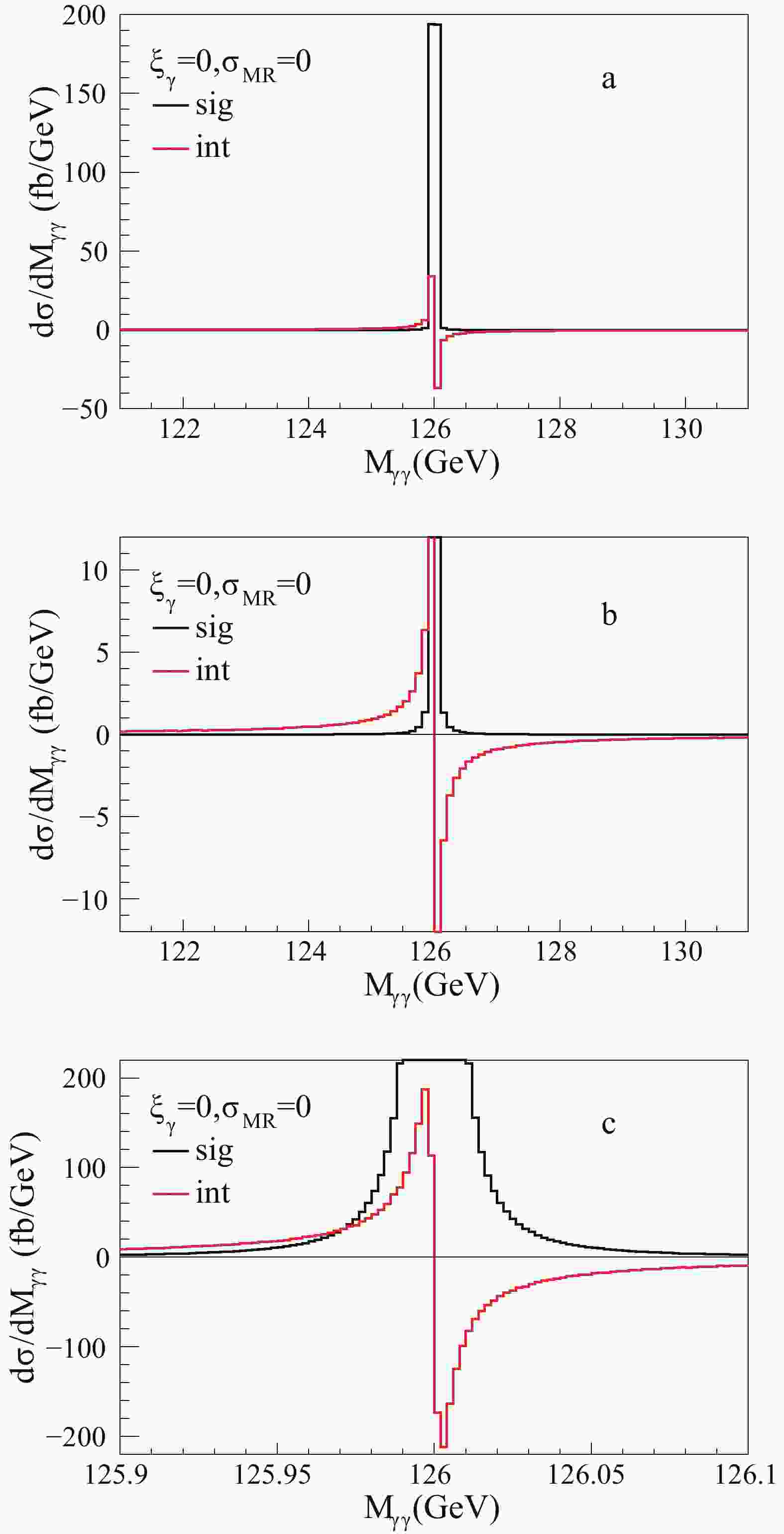
Fig. 1 shows the theoretical line shapes of the signal (a sharp peak shown in the black histogram) and the interference (a peak and dip shown in the red histogram); Fig. 1(a) is the overall plot, Fig. 1(b) and Fig. 1(c) are close-ups. As shown in Fig. 1(a) and Fig. 1(b), the signal has a mass peak that is about four times larger than the interference. The mass peak of the interference is wider and has a much longer tail. The resonance region
$ [125.9, 126.1] $ GeV is shown in Fig. 1(c) with a bin width reduced from 100 MeV to 2 MeV. The signal exceeds the interference from the energy$ M_{\gamma\gamma}\approx M_H-10\times\Gamma_H $ . After integrating,$ A_{\rm{int}}^{\rm{SM}} $ is 36% , as shown in Table 1, which is quite large. As the smearing from the mass resolution (MR) is not considered yet, we denote this case as$ \sigma_{\rm{MR}} = 0 $ .$\sigma_{\rm{MR}}$ (GeV)

$A^{\rm{SM}}_{\rm{int}}$ denominator (fb)

$A^{\rm{SM}}_{\rm{int}}$ numerator (fb)

$A^{\rm{SM}}_{\rm{int}}$ (%)

0 39.3 14.3 36.3 1.1 39.3 4.0 10.2 1.3 39.3 3.7 9.4 1.5 39.3 3.4 8.6 1.7 39.3 3.1 7.9 1.9 39.3 2.8 7.2 Table 1.
$A^{\rm{SM}}_{\rm{int}}$ values for different mass resolution widths.$\sigma_{\rm{MR}}=0$ represents the theoretical case before Gaussian smearing.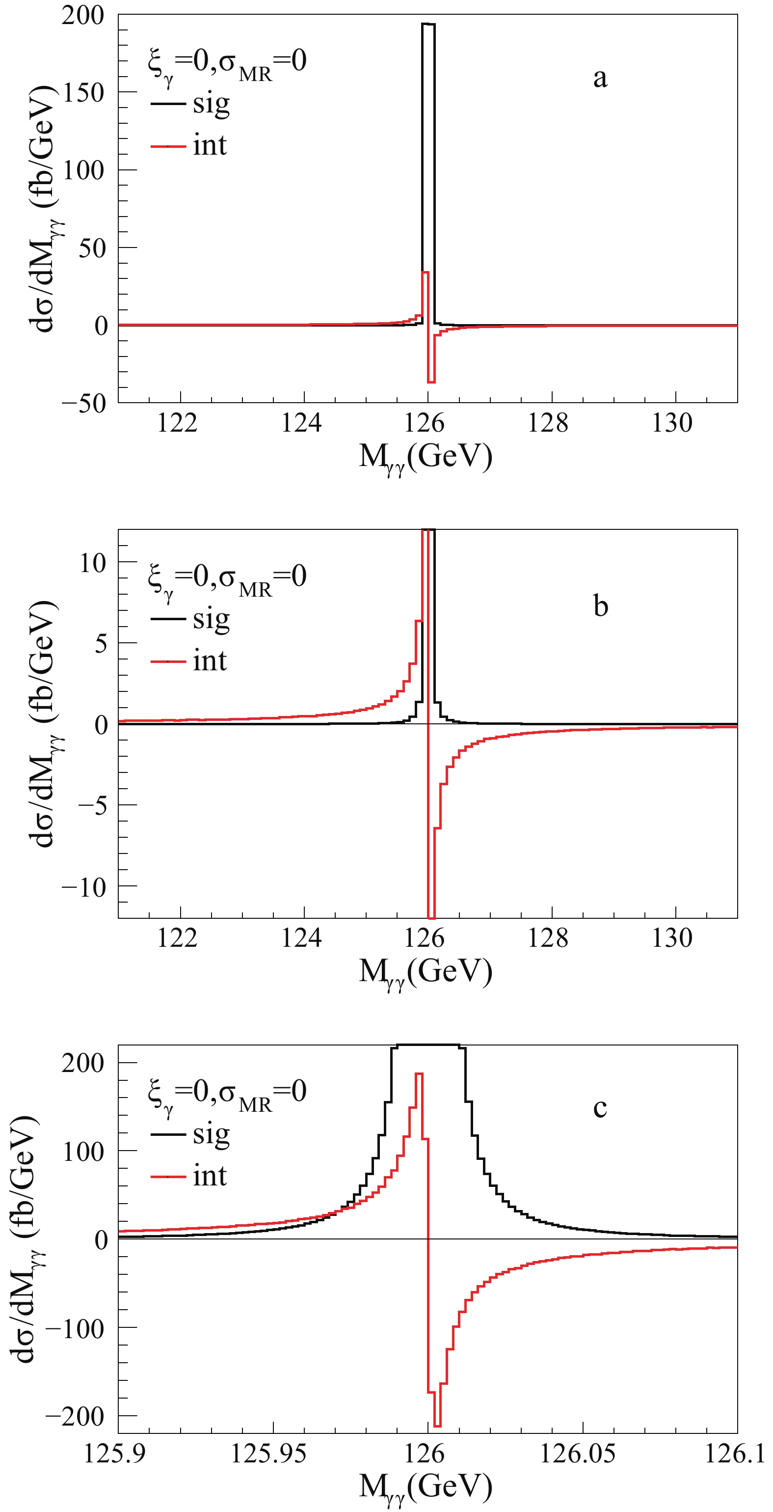
Figure 1. (color online) Diphoton invariant mass
$ {M_{\gamma \gamma }}$ distribution of the signal and the interference given by Eq. (9) and (10).$ {\xi _\gamma }$ = 0 represents the SM case,$ {\sigma _{{\rm{MR}}}}$ = 0 represents the theoretical distribution before Gaussian smearing. (a) is the overall plot, (b) and (c) are close-ups.The invariant mass of the diphoton
$ M_{\gamma\gamma} $ has a mass resolution of about$ 1\sim2 $ GeV in the CMS experiment [41]. For simplicity we include the mass resolution by convoluting the histograms with a Gaussian function with widths$ \sigma_{\rm{MR}} = 1.1, 1.3, 1.5, 1.7, 1.9 $ GeV. This convolution procedure is also called Gaussian smearing. Fig. 2 shows the line shapes after Gaussian smearing with$ \sigma_{\rm{MR}} = 1.5 $ GeV. The sharp peak of the signal becomes a wide bump (the black histogram), while the peak and dip of the interference are also wider. As they cancel each other near$ M_H $ , the former peak and dip take a moderately antisymmetric shape around$ M_H $ (the red histogram).$ A_{\rm{int}}^{\rm{SM}} $ after Gaussian smearing is thus reduced, and ranges from 10.2% to 7.2% when$ \sigma_{\rm{MR}} $ increases from 1.1 to 1.9 GeV, as shown in Table 1.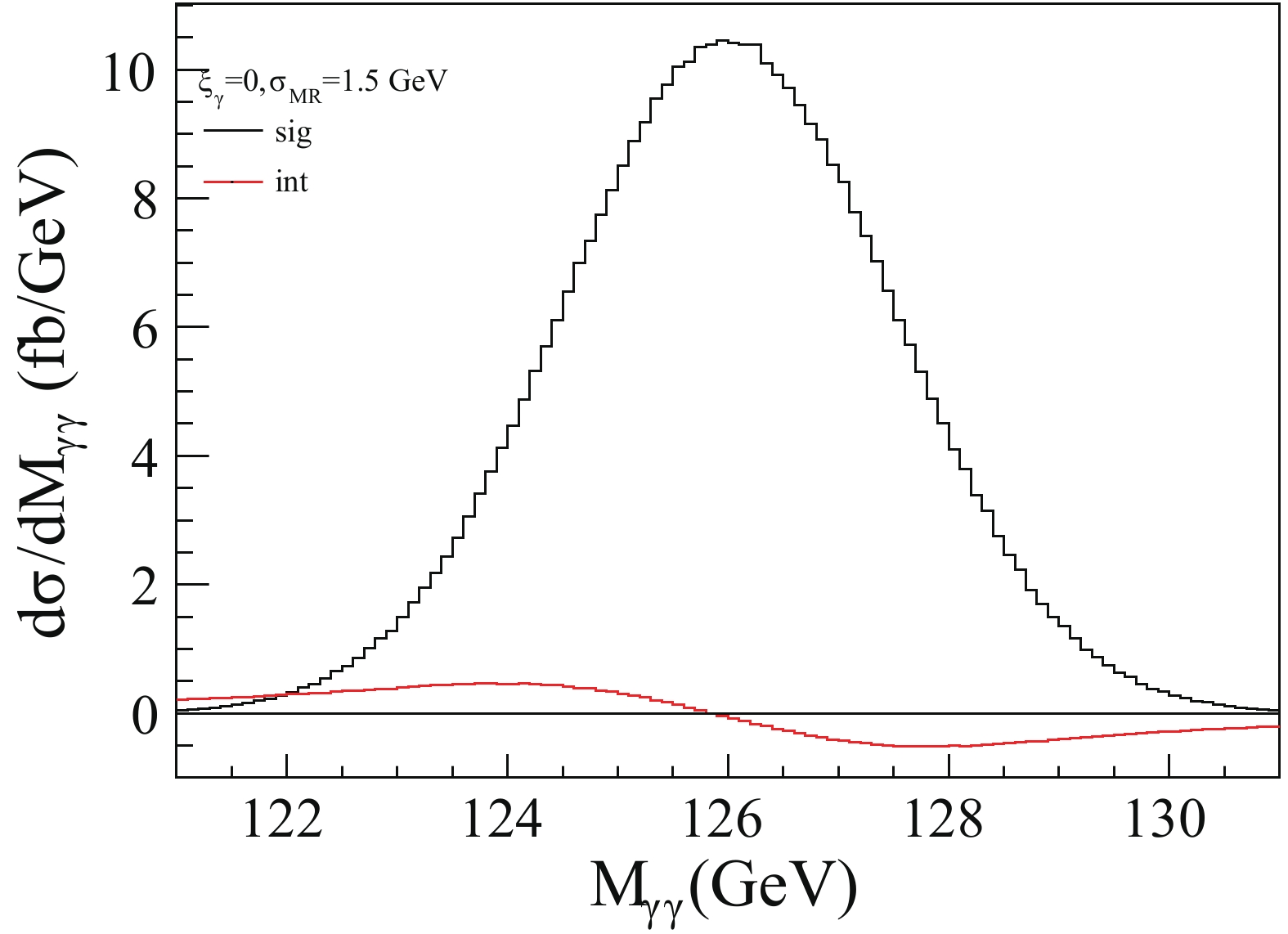
Figure 2. (color online) Diphoton invariant mass
$ {M_{\gamma \gamma }}$ distribution after Gaussian smearing with mass resolution width$ {\sigma _{{\rm{MR}}}}$ = 1.5 GeV. -
Fig. 3 shows the interference line shapes when
$ \xi_\gamma = 0, \pi, $ $ \pi/2 $ and$ \sigma_{\rm{MR}} = 1.5 $ GeV. The blue histogram ($ \xi_\gamma = \pi $ , sign-reversed CP-even$ H\gamma\gamma $ coupling) is almost opposite to the red histogram ($ \xi_\gamma = 0 $ , SM), and they correspond to the minimum and maximum of$ A_{\rm{int}} $ . The black dashed histogram ($ \xi_\gamma = \pi/2 $ , CP-odd$ H\gamma\gamma $ coupling) looks like a flat line (actually with some tiny fluctuations from the simulation), and corresponds to zero of$ A_{\rm{int}} $ . Fig. 4 shows$ A_{\rm{int}} $ and its absolute statistical error$ \delta A_{\rm{int}} $ . The statistical error is estimated using an integrated luminosity of 30 fb−1, and the efficiency of the detector is assumed to be one.$ \delta A_{\rm{int}} $ decreases as$ A_{\rm{int}} $ becomes smaller. However, the relative statistical error$ \delta A_{\rm{int}}/A_{\rm{int}} $ increases quickly and becomes very large as$ A_{\rm{int}} $ approaches zero. In SM ($ \xi_\gamma = 0 $ in Fig. 4), the relative statistical error$ \delta A_{\rm{int}}/A_{\rm{int}} $ is about 18% with the assumption of zero correlation between symmetric and antisymmetric cross-sections.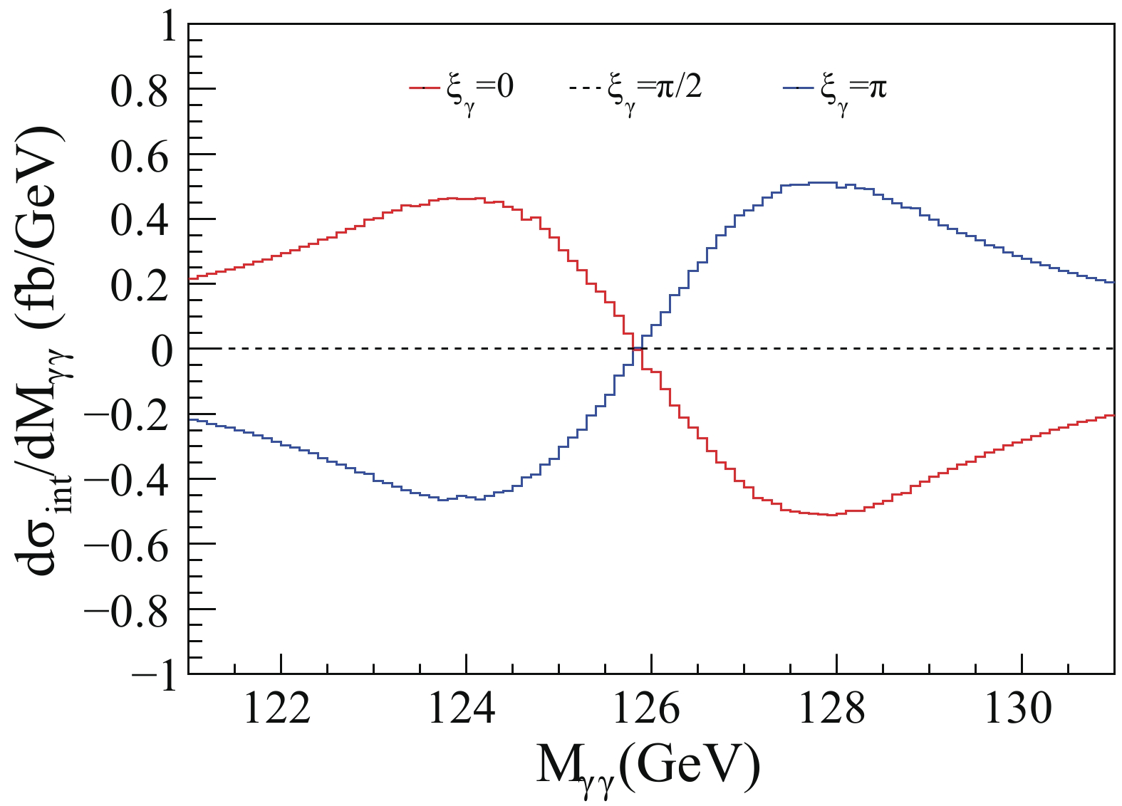
Figure 3. (color online) Diphoton invariant mass
$M_{\gamma\gamma}$ distribution of the interference after Gaussian smearing with$\sigma_{\rm{MR}}=1.5$ GeV for$\xi_\gamma=0, ~\pi, ~\pi/2$ .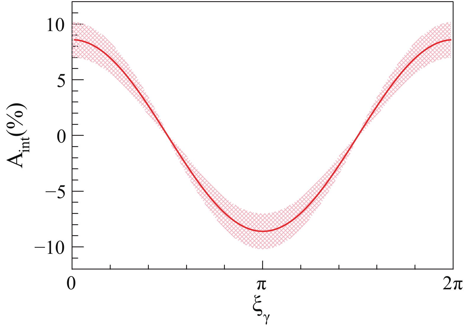
Figure 4. (color online)
$A_{\rm{int}}$ values (red line) and their statistical errors (shade) for different phase$\xi_\gamma$ . -
In the CMS or ATLAS experiments, the
$ \gamma\gamma $ mass spectrum is fitted by a signal function and a background function. To consider the interference effect, the antisymmetric line shape should also be included. That is, instead of a Gaussian function (or a double-sided Crystal Ball function) as the signal in the LHC experiments [41, 42], a Gaussian function (or a double-sided Crystal Ball function) plus an asymmetric function should be used as the modified signal, while the background should be kept the same.To see whether or not the asymmetric line shape could be extracted, we carry out a fit of the modified signal from two background-subtracted data samples. As the background fluctuation would be dealt similarly as in the real experiment, we ignore it here for simplicity. One data sample is from the CMS experiment Ref. [41], from where we take 10 data points with their errors between
$ [121, 131] $ GeV in the background-subtracted$ \gamma\gamma $ mass spectrum for 35.9 fb−1 integrated luminosity with proton-proton collision energy of 13 TeV (see Fig. 13 in Ref. [14]). The fitting function is given as$ f(m) = c_1\times f_{\rm{sig}}(m-\delta m)+c_2\times f_{\rm{int}}(m-\delta m), $

(14) where
$ c_1, c_2, \delta m $ are the fitting parameters, m is the$ \gamma\gamma $ invariant mass, the functions$ f_{\rm{sig}}(m), f_{\rm{int}}(m) $ are evaluated from the two histograms in Fig. 2 and they describe the signal and interference. Fig. 5 shows the fit result of the CMS data, in which the crosses represent CMS data with their errors, the red solid line is the combined function, and the black dashed line and the blue dotted line are the signal and interference components, respectively. The black dashed line is almost the same as the red solid line, while the blue dotted line is almost flat. The fitting parameter$ c_2 $ for the interference component has a huge uncertainty that is even larger than the central value of$ c_1 $ , which indicates that it is hard to extract the interference component from 35.9 fb-1 of CMS data. For comparison, we simulate a pseudo-data sample from the combined histogram in Fig. 2, which is normalized to about 80 times the amount of CMS data (corresponding to an integrated luminosity of 3000 fb-1), with a bin width of$ 0.5 $ GeV and Poission fluctuation. The result of the fit is shown in Fig. 6, where the red solid line is shifted from the black dashed line, and the blue dotted line can be clearly distinguished.$ c_1 $ and$ c_2 $ are fitted as$ c_1 =0.999\pm $ $ 0.002 $ ,$ c_2 = 0.947 \pm 0.028 $ , which are consistent with their SM expected value 1 and deduce to a relative error of$ A_{int}\sim $ 3% according to the error propagation formula. Even though this fitting result looks quite good, it can only reflect that the antisymmetric lineshape could be extracted out when no contamination comes from systematic error. Furthermore, our study shows that the optimal fitting strategy is taking Higgs mass as a free parameter together with$ c_1 $ and$ c_2 $ . Although$ M_H $ has been measured in many channels, its fluctuation is usually too large to get a converged fitting if we take it as a known input value.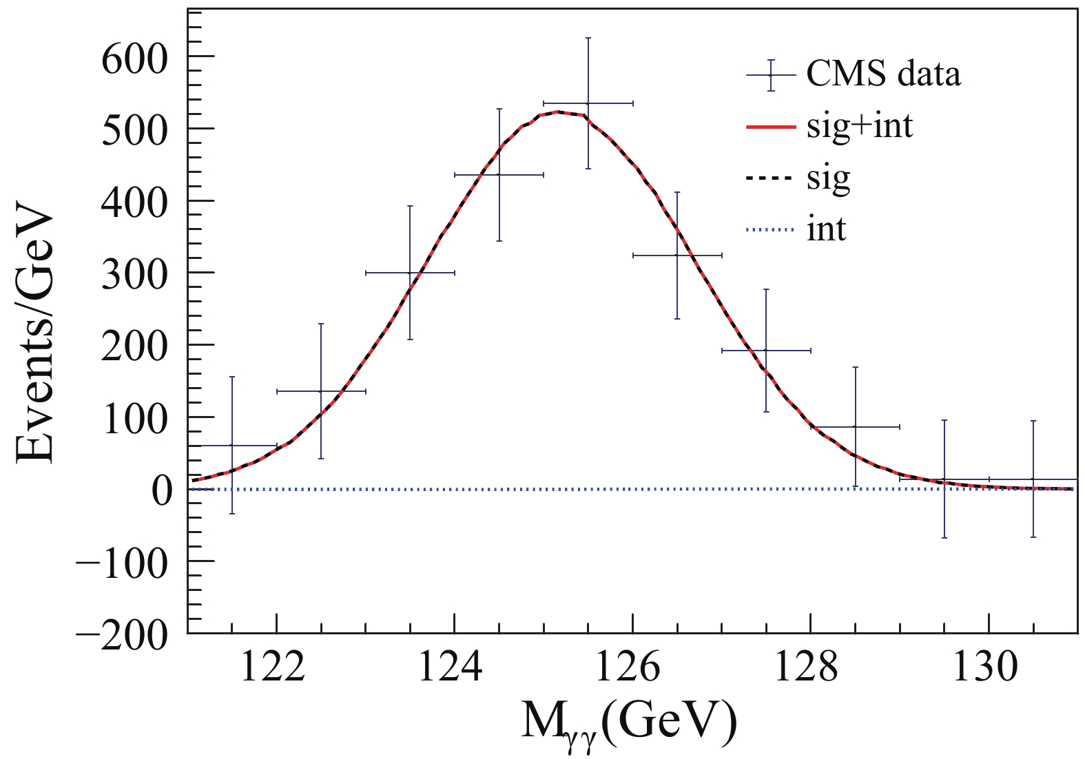
Figure 5. (color online) Fit of the background-substracted CMS data sample. The crosses represent CMS data from Ref. [41]. The red solid line is the combined function, the black dashed line and the blue dotted line represent the signal and interference components, respectively.
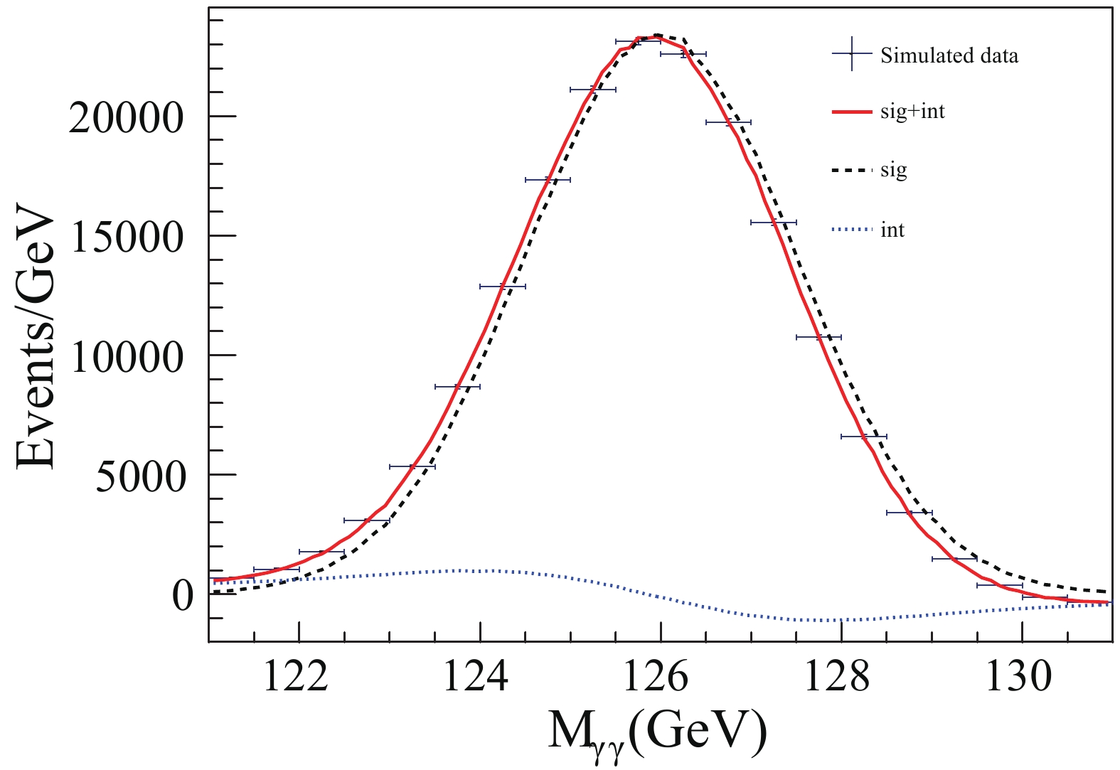
Figure 6. (color online) Fit of the simulated data sample. The crosses represent simulated data from the combined histogram in Fig. 2 normalized to an integrated luminosity of 3000 fb−1. The red solid line is the combined function, the black dashed line and the blue dotted line represent the signal and interference components, respectively.
In contrast, a simulation that also studied the interference effect including the systematic errors has been carried out by the ATLAS collaboration for the HL-LHC with an integrated luminosity of 3000 fb−1 [43]. In that simulation, the mass shift of the Higgs boson caused by the interference effect has been studied with different assumptions for the Higgs width. A pseudo-data was produced by smearing a Breit-Wigner distribution with a model of the detector resolution, and the interference effect was described by the shift of the smeared Breit-Wigner distribution. Based on fitting, the mass shift of the Higgs from the interference effect was estimated to be
$ \Delta m_H = -54.4 $ MeV for the SM case, and the systematic error of the mass difference was about 100 MeV. If this result is used to estimate the mass shift effect for the non-SM$ \xi_\gamma\ne 0 $ cases, ($ \xi_\gamma = \pi/2 $ corresponds to a zero mass shift, and$ \xi_\gamma = \pi $ to a reverse mass shift of$ \Delta m_H = +54.4 $ MeV, as shown in Fig. 3), then the largest deviation of the mass shift from the SM case is$ 2\times 54.4 $ MeV (when$ \xi_\gamma = \pi $ ), which is almost covered by the systematic error of$ 100 $ MeV. Therefore, the non-SM$ \xi_\gamma\ne 0 $ cases can not be distinguished using this mass shift effect. Nevertheless, it is worth noting that the antisymmetric line shape of the theoretical interference effect is quite different from the shift of two smeared Breit-Wigner distributions in the ATLAS simulation [43], especially in the region far from the Higgs peak, where the antisymmetric line shape of the interference effect has a long flat tail while the Breit-Wigner distribution falls quickly. The authors of the ATLAS study have also noted this difference and have planned to include it in their new search [43]. -
In the above study,
$ Hgg $ coupling is assumed to be SM-like. Furthermore, the observable$ A_{\rm{int}} $ could also be used to probe CP violation in$ Hgg $ coupling. In this section, we add one more parameter,$ \xi_g $ , to describe CP violation in$ Hgg $ coupling, and study$ A_{\rm{int}} $ following the same procedure as above.Based on Eq. (1), the parameter
$ \xi_g $ to describe CP violation in$ Hgg $ coupling is added, and the effective Lagrangian is modified as$ \begin{split} {\cal L}_{\rm h} = & \frac{c_\gamma \cos\xi_\gamma}{v}\; h\, F_{\mu\nu} F^{\mu\nu} + \frac{c_\gamma \sin\xi_\gamma}{2v}\; h\, F_{\mu\nu}{\tilde{F}}^{\mu\nu} \\ &+\frac{c_g \cos\xi_g}{v}\; h\, G^a_{\mu\nu}G^{a\mu\nu} \\&+ \frac{c_g \sin\xi_g}{2v}\; h\, G^a_{\mu\nu}{\tilde{G}}^{a\mu\nu}\; . \end{split}$

(15) The helicity amplitude in Eq. (7) and the differential cross-section of the interference in Eq. (10) should be changed correspondingly, and become
$ \begin{split} {\cal M} =& -{\rm e}^{-{\rm i} h_1 \xi_g}{\rm e}^{-{\rm i} h_3\xi_\gamma}\delta^{h_1h_2}\delta^{h_3h_4}\delta^{a b}\frac{M^4_{\gamma\gamma}}{v^2} \frac{4c_gc_\gamma}{M^2_{\gamma\gamma}-M^2_H+iM_H\Gamma_H} \\ &+ 4\alpha\alpha_s\delta^{a b}\sum_{f = u, d, c, s, b} Q^2_f {\cal A}_{\rm{box}}^{h_1 h_2 h_3h_4}\;, \end{split}$

(16) $ \begin{split} \frac{{\rm d}\sigma_{\rm{int}}}{{\rm d}M_{\gamma\gamma}} \propto& \frac{(M^2_{\gamma\gamma}-M^2_H)\operatorname{Re}\left(c_g c_\gamma \right) +M_H\Gamma_H \operatorname{Im}\left(c_g c_\gamma \right) } {(M^2_{\gamma\gamma}-M^2_H)^2+M^2_H\Gamma^2_H} \\ & \times \int {\rm d}z[\cos(\xi_g+\xi_\gamma){\cal A}_{\rm{box}}^{++++}+\cos(\xi_g-\xi_\gamma){\cal A}_{\rm{box}}^{++--}]\; . \end{split}$

(17) Then,
$ A_{\rm{int}}^{\rm{SM}}\equiv A_{\rm{int}}(\xi_g = 0, \xi_\gamma = 0) $ and$ \begin{split} A_{\rm{int}}(\xi_g, \xi_\gamma) =& A_{\rm{int}}^{\rm{SM}}\\&\times \frac{\int {\rm d}z[\cos(\xi_g+\xi_\gamma){\cal A}_{\rm{box}}^{++++}+\cos(\xi_g-\xi_\gamma){\cal A}_{\rm{box}}^{++--}]}{\int {\rm d}z[{\cal A}_{\rm{box}}^{++++}+{\cal A}_{\rm{box}}^{++--}]}\;, \end{split}$

(18) where the integral can be calculated numerically once the region of z integration is given. For example, if the pseudorapidity of
$ \gamma $ is required to be$ |\eta^{\gamma}|<2.5 $ , that is,$ z\in [-0.985, 0.985] $ , the integral$ \int {\rm d}z {\cal A}_{\rm{box}}^{++--}\approx -9 $ , and Eq. (18) can be simplified as$ A_{\rm{int}}(\xi_g, \xi_\gamma)\approx A_{\rm{int}}^{\rm{SM}}\times \frac{2\cos(\xi_g+\xi_\gamma)-9\cos(\xi_g-\xi_\gamma)} {-7}\; . $

(19) $ A_{\rm{int}}(\xi_g, \xi_\gamma) $ thus has the maximum and minimum about 1.6 times that of$ A_{\rm{int}}^{\rm{SM}} $ . If$ \xi_g = 0 $ ,$ A_{\rm{int}}(\xi_g = 0, \xi_\gamma) $ degenerates to$ A_{\rm{int}}(\xi_\gamma) $ in Eq. (13). In contrast, if$ \xi_\gamma = 0 $ ,$ A_{\rm{int}}(\xi_g) = A_{\rm{int}}^{\rm{SM}}\times \cos(\xi_g), $

(20) which shows the same dependence as
$ A_{\rm{int}}(\xi_\gamma) $ on$ \xi_\gamma $ when$ \xi_g = 0 $ as in Eq. (13). Hence, a CP violating$ Hgg $ coupling can cause similar deviation of$ A_{\rm{int}} $ from$ A_{\rm{int}}^{\rm{SM}} $ as a CP violating$ H\gamma\gamma $ coupling, and a single observed$ A_{\rm{int}} $ can not distinguish between them since there are two free parameters for one observable.Fig. 7 shows the interference line shapes for different
$ \xi_g, \; \xi_\gamma $ . The red histogram ($ \xi_g = 0, \; \; \xi_\gamma = 0 $ ) represents the SM case; the magenta histogram$ \left(\xi_g = \displaystyle\frac{\pi}{2}, \; \; \xi_\gamma = \displaystyle\frac{\pi}{2}\right) $ has the largest$ A_{\rm{int}} $ ; the cyan histogram$\left( \xi_g = \displaystyle\frac{\pi}{2}, \; \; \xi_\gamma = \displaystyle\frac{3\pi}{2} \right)$ corresponds to the smallest$ A_{\rm{int}} $ ; and the black histogram is for the case of$ \xi_g = 0, \; \; \xi_\gamma = \displaystyle\frac{\pi}{2} $ with$ A_{\rm{int}} $ equal to zero. In the general case where both$ \xi_g, \; \xi_\gamma $ are free parameters,$ A_{\rm{int}}(\xi_g, \; \xi_\gamma) $ has a wider range of values than$ A_{\rm{int}}(\xi_\gamma) $ , which makes it easier to probe in future experiments.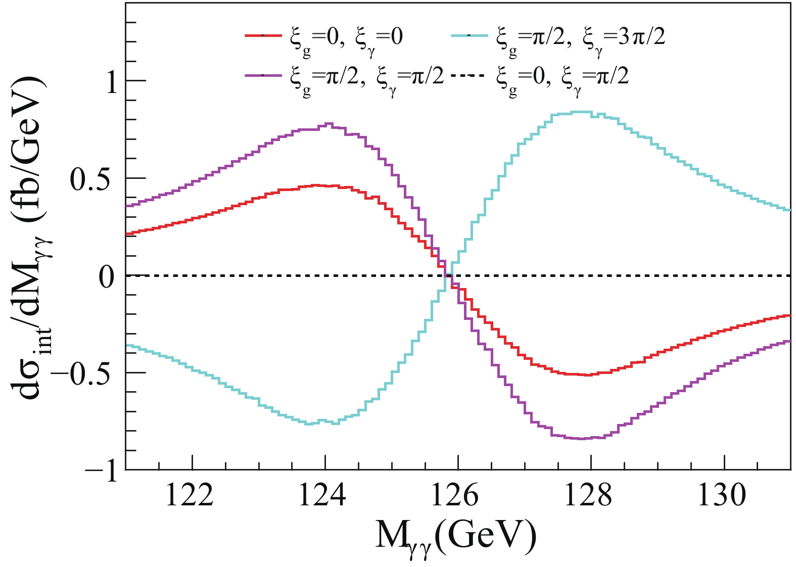
Figure 7. (color online) Diphoton invariant mass
$M_{\gamma\gamma}$ distribution of the interference after Gaussian smearing in various$\xi_g, ~\xi_\gamma$ cases. -
The diphoton mass distribution from the interference between
$ gg\to H \to \gamma\gamma $ and$ gg\to \gamma\gamma $ to leading order is almost antisymmetric around$ M_H $ and we propose a sign-reversed integral around$ M_H $ to get its contribution. After dividing the integral by the cross-section of the Higgs signal, we get the observable$ A_{\rm{int}} $ . In SM, the theoretical value of$ A_{\rm{int}} $ , before taking into account the mass resolution, is ~ 39%. After considering the mass resolution of$ \sim1.5 $ GeV,$ A_{\rm{int}} $ is reduced, but still could be as large as 10%. CP violation in$ H\gamma\gamma $ could change$ A_{\rm{int}} $ from 10% to -10% , depending on the CP violation phase$ \xi_\gamma $ . In the general framework of CP violating$ H\gamma\gamma $ and$ Hgg $ couplings,$ A_{\rm{int}} $ could have a larger value, ~ ±16%. However, due to the systematic and statistical errors which are both ~ 10% in the current experiments at the LHC, it is difficult to extract the antisymmetric line shape. Even with future high luminosities, the large systematic error is still a serious obstacle.
Probing the CP violating Hγγ coupling using interferometry
- Received Date: 2019-02-15
- Accepted Date: 2019-04-22
- Available Online: 2019-07-01
Abstract: The diphoton invariant mass distribution from the interference between


 DownLoad: