Statistical method in quark combination model

Most hadronization models, such as the Lund string model [1–4] or the coalescence/recombination models [5–21] in electron-positron and hadron-hadron collisions, assume that a hadron is formed by quarks and antiquarks in the neighborhood of phase space. Normally, the phase space can be decomposed into the longitudinal and transverse directions. The longitudinal phase space plays a particular role. For example, in the Lund model, a string is formed between a quark and an antiquark moving back to back, which is an object with only one spatial dimension, i.e., with only the longitudinal phase space. A quark-antiquark pair is produced as the result of the string breaking into two pieces. The process of string breaks continues until it is terminated at a lowest energy scale. The transverse momentum space of the excited quark-antiquark pair is rather limited and can be described by the exponentially suppressed function of the transverse momentum. In relativistic heavy-ion collisions, the longitudinal phase space remains dominant, although transverse expansion is significant.

The quark combination model developed by the Shandong group (SDQCM) [9–11, 22–35] is a kind of exclusive or statistical hadronization model, which differs from the Lund string model and the coalescence model. The model first takes the constituent quark degrees of freedom as an effective description for the strongly-interacted quark gluon system at hadronization. Subsequently, the model adopts a quark combination rule (QCR) to combine the quarks and antiquarks in the neighborhood of the longitudinal phase space into baryons and mesons. Since the longitudinal phase space is easily described by the momentum rapidity, the correlation in rapidity is the basis of the QCR. This type of QCR in SDQCM has successfully explained many data of hadronic production in $e^{+}e^{-}$ and pp collisions [24, 25, 36, 37] and rapidity distributions of hadrons in heavy-ion collisions [26, 27, 31, 38].

The probability distributions of the particle numbers of baryons, antibaryons, and mesons is an important observable in high energy collisions and is closely related to hadronization dynamics. Especially, the particle number distributions are essential to the search for the critical end point of the QCD phase diagram in relativistic heavy-ion collisions [39–43]. In this study, we propose a new method to solve the baryon and meson number distribution in the context of the QCR in the SDQCM. The new method is significantly simpler and easier to generalize to more sophisticated cases than the original one [44]. We followingly employ these formula to calculate the multiplicity distribution and ratios of cumulants for net protons in relativistic heavy-ion collisions.

The paper is organized as follows. In Sec. 2, we briefly present the original QCR in the SDQCM. Then, we apply the generating function method to solve the particle number probability of baryons, antibaryons, and mesons for a given number of quarks and antiquarks. In Sec. 3, we generalize the original QCR and derive the corresponding particle number probability of baryons, antibaryons, and mesons using the generating function method. In Sec. 4, we compare the numerical difference between the original QCR and the generalized QCR in terms of moments of the antibaryon number. In Sec. 5, we formulate the fluctuation and correlation of identified hadrons. In Sec. 6 and 7, we study the effects of the quark number fluctuation and resonance decays. In Sec. 8, we provide an illustrative example of applying the QCR and generalized QCR to calculate the ratios of cumulants for net protons in heavy-ion collisions and compare it with the obtained data. Finally, we provide a summary and discussions in Sec. 9.

Because of the non-perturbative QCD feature, the transition from quarks and/or gluons to hadrons is not solved from the first principle, and it is presently only described by the phenomenological models. Inspired by the simple and effective description of the constituent quark model in explaining the static property of hadrons, SDQCM assumes the constituent quarks and antiquarks as effective degrees of freedom for the strongly-interacting quarks and gluons at hadronization ,and therefore builds a simple hadronization phenomenology by the combination of these constituent quarks and antiquarks into hadrons. We emphasize that there are explicit experimental signals for such constituent quark degrees of freedom in high energy collisions, such as the quark number scaling property of elliptic flows and the transverse momentum spectra for hadrons observed in recent years [45–50]. A phenomenological quark combination rule was proposed in Ref. [22] to describe the combination of these constituent quarks and antiquarks in a one-dimensional phase space and can successfully describe the data of yields and momentum distributions of hadrons in high-energy reactions [24–27, 31, 36–38]. In this section, we use the generating function method to solve the probability distribution for the number of baryons, antibaryons, and mesons formed by QCR.

In the QCM, $N_{q}$ quarks and $N_{\bar{q}}$e antiquarks generated in an event are placed into a queue and then allowed to combine into hadrons one by one following the quark combination rule (QCR) [22]. QCR is based on the basic property of QCD. A $q\overline{q}$ pair may occur in a color octet with a repulsive interaction or a singlet with a attractive interaction. If $q\overline{q}$ is adjacent in phase space, $q\overline{q}$ will have sufficient time or opportunity to be in a color state and hadronize into a meson. For a qq pair, it may be in a sextet or an antitriplet. If its nearest neighbor is a q in phase space, they can hadronize into a baryon. If the neighbor of qq is a $\overline{q}$, $q\overline{q}$ will win the competition to form a meson and leave a q to combine with other quarks and/or antiquarks. This is because the attraction strength of the singlet for $q\bar{q}$ is two times that of the antitriplet for qq (via counting the color factor in the one-gluon exchange case). The original QCR proposed in Ref. [22] reads:

1. Check if there are partons in the queue. If there are no partons, the process ends. Otherwise, start from the first parton (q or $\overline{q}$) in the queue and proceed to the next step.

2. Look at the second parton. If there is no second parton, the process ends. Otherwise, if the baryon number of the second parton in the queue is different from the first one, i.e., the first two partons are either $q\overline{q}$ or $\overline{q}q$r, they combine into a meson and are removed from the queue, repeat step 1; Otherwise, if they are either qq or $\overline{q}\overline{q}$, proceed to the next step.

3. Look at the third parton. If there is no third parton, the process ends. Otherwise, if the third parton is different in the baryon number from the first one, the first and third parton form a meson and are removed from the queue, repeat step 1; Otherwise, if the first three partons combine into a baryon or an antibaryon and are removed from the queue, go to step 1.

The following example demonstrates the function of the QCR.

In relativistic heavy-ion collisions, the longitudinal rapidity space is predominant, and the rapidity density of quarks and antiquarks is quite large. Therefore, it is suitable and straightforward to apply such a QCR in one-dimensional longitudinal rapidity space. However, it is quite complicated in three dimensional phase space, because one can not easily define a particular hadronization order to apply QCR [51].

We consider the system consisting of $N_{q}$ quarks and $N_{\bar{q}}$ antiquarks stochastically populated in one-dimensional phase space. After combination by QCR, there are $N_{B}$ baryons, $N_{\bar{B}}$ antibaryons, and $N_{M}$ mesons formed, and $N_{r}$ quarks and $N_{\bar{r}}$ antiquarks left. There are only five different configurations with $(N_{r},N_{\bar{r}}) = (0,0),(0,1), (1,0),(2,0),$ and $(0,2)$. The quark number conservation gives

The outcome of implementing the QCR to the queue of $N_{q}$ quarks and $N_{\bar{q}}$ antiquarks yields a group of numbers $(N_{M},N_{B},N_{\bar{B}},N_{r},N_{\bar{r}})$. The queue $(N_{M},N_{B},N_{\bar{B}},0,0)$ can be reached by one of the following ways of adding one q or $\bar{q}$ to the end of the other four queues with a smaller number of quarks and antiquarks

We use $F(N_{M},N_{B},N_{\bar{B}},N_{r},N_{\bar{r}})$ to denote the number of different queues for a given group $(N_{M},N_{B},N_{\bar{B}},N_{r},N_{\bar{r}})$. We define $F(0,0,0,0,0) = 1$ and $F(N_{M},N_{B},N_{\bar{B}},N_{r},N_{\bar{r}}) = 0$ for the case that any $N_{M}$, $N_{B}$, $N_{\bar{B}}$, $N_{r}$, and $N_{\bar{r}}$ are negative. Under the constraint of Eq. (2), the sum of $F(N_{M},N_{B},N_{\bar{B}},N_{r},N_{\bar{r}})$ over all different groups of $(N_{M},$ $N_{B},N_{\bar{B}},N_{r},N_{\bar{r}})$ should be

where $\delta_{i,j} = 1$ if $i = j$ and $\delta_{i,j} = 0$ if $i\neq j$.

For non-zero $N_{r}$ and $N_{\bar{r}}$, $F(N_{M},N_{B},N_{\bar{B}},N_{r},N_{\bar{r}})$ has a property

Proof of Property. We first take $(N_{r},N_{\bar{r}}) = (1,0)$ as an example. We note that the queue yielding $(N_{M},N_{B},N_{\bar{B}},1,0)$ can be achieved in two ways: (a) adding q to the end of the queue with $(N_{M},N_{B},N_{\bar{B}},0,0)$; (b) adding $\bar{q}$ to the end of the queue with $(N_{M}-1,N_{B},N_{\bar{B}},2,0)$, which can further be obtained from the queue with $(N_{M}-1,N_{B},N_{\bar{B}},1,0)$ by adding a q at the end. Thus, we obtain the recursive relation

Solving the above equation recursively, we obtain Eq. (5), where we used $F(0,N_{B},N_{\bar{B}},1,0) = F(0,N_{B},N_{\bar{B}},0,0)$. The proof of the case $(N_{r},N_{\bar{r}}) = (2,0)$ is straightforward, because the queue yielding $(N_{M},N_{B},N_{\bar{B}},2,0)$ can be only obtained from the queue with $(N_{M},N_{B},N_{\bar{B}},1,0)$ by adding a q at the end. The proof for the cases $(N_{r},N_{\bar{r}}) = (0,1)$ and $(N_{r},N_{\bar{r}}) = (0,2)$ is similar.

Using properties in Eq. (5) and Eq. (3), we obtain

We make the replacement $N_{M}\rightarrow N_{M}-1$ in the above equation and take the difference between the two. Finally, we use Eq. (5) to obtain the recursive equation for $F(N_{M},$$N_{B},N_{\bar{B}},0,0)$

where $N_{M}\geqslant0$, $N_{B}\geqslant0$, $N_{\bar{B}}\geqslant0$ excluding two cases $(N_{M},N_{B},N_{\bar{B}},N_{r},N_{\bar{r}}) = (0,0,0,0,0),(1,0,0,0,0)$, which we have $F(0,0,0,0,0) = 1$ by definition and $F(1,0,0,0,0) = 2$ by simple counting.

First, we consider a special simple case: $N_{M}>1$, $N_{B} = N_{\bar{B}} = 0$, $N_{r} = N_{\bar{r}} = 0$. Eq. (8) is simplified to

which immediately leads to the solution

for $N_{M}\geqslant1$ with $F(1,0,0,0,0) = 2$.

Now, we consider the general case for $F(N_{M},N_{B},N_{\bar{B}},0,0)$ with $N_{M}\geqslant0$, $N_{B}\geqslant0$, $N_{\bar{B}}\geqslant0$. We define the generating function

and $F(N_{M},N_{B},N_{\bar{B}},0,0)$ is the coefficient of $x^{N_{M}}y^{N_{B}}z^{N_{\bar{B}}}$ in the polynomial expansion of $A(x,y,z)$, once solved.

To solve $A(x,y,z)$, we define a partial generating function

Inserting Eq. (8) for $N_{M}\geqslant1$, we obtain

In a special case with $N_{B} = 0$, we obtain

where we used Eq. (10) and assumed that $3|x|<1$. In the same way, we obtain

We also obtain two sum rules

where the convergent region is $|y|,|z|<|1-3x|$.

We now multiply Eq. (13) by $y^{N_{B}}z^{N_{\bar{B}}}$ and take a sum over $N_{B}$ from 1 to infinity, and $N_{\bar{B}}$ from 1 to infinity. By noticing $A(x,y,z) = \sum_{N_{B} = 0}^{\infty}\sum_{N_{\bar{B}} = 0}^{\infty}A(x;N_{B},N_{\bar{B}})y^{N_{B}}z^{N_{\bar{B}}}$ and employing Eqs. (16) and (17), we solve the generating function as

To obtain $F(N_{M},N_{B},N_{\bar{B}},0,0)$, we first extract the coefficient of $z^{N_{\bar{B}}}$

Then, we extract the coefficient of $y^{N_{B}}$ in $C(z^{N_{\bar{B}}})$ as

where we apply

for $n>0$ and $|w|<1$. Finally, we extract the coefficient of $x^{N_{M}}$ in $C(z^{N_{\bar{B}}}y^{N_{B}})$, i.e.,

which yields the final result for

Eq. (23) is the result of QCR in Sect. 2.1 and was first given in Ref. [44] by mathematical induction and the traditional combination method. The current derivation is a simplified one, based on the recursive equation and the method of generating functions. The probability of forming $N_{M}$ mesons, $N_{B}$ baryons, and $N_{\bar{B}}$ antibaryons in a quark system with $N_{q}$ quarks and $N_{\bar{q}}$ antiquarks is given by

Here, we have removed the label '0,0' from $P(N_{M},N_{B},N_{\bar{B}})$, since this is the real case in hadronization.

The ratio of baryons to mesons (B/M) given by QCR in Sect. 2.1 is larger than the observation of heavy-ion collisions [52, 53]. To suppress the B/M ratio, we can generalize the QCR in Sect. 2.1 to decrease the formation probability of baryons relative to mesons. The generalized QCR (gQCR) reads:

1. Check if there are partons in the queue. If there are no partons, the process ends. Otherwise, start from the first parton and proceed to the next step.

2. Look at the second parton. If there is no second parton, the process ends. Otherwise, if the baryon number of the second parton is different from the first one, i.e., the first two partons are either $q\overline{q}$ or $\overline{q}q$, they combine into a meson and are removed from the queue, repeat step 1; Otherwise if they are either qq or $\overline{q}\overline{q}$, proceed to the next step.

3. Look at the third parton. If there is no third parton, the process ends. Otherwise, if the baryon number of the third parton is different from the first one, the first and third parton form a meson and are removed from the queue, repeat to step 1; Otherwise if the first three partons are either qqq or $\overline{q}\overline{q}\overline{q}$, proceed to next step.

4. Look at the fourth parton. If there is no fourth parton, the first three partons form a baryon or an antibaryon and the process ends. Otherwise, if the baryon number of the fourth parton is different from the first one, the first and fourth parton form a meson and are removed from the queue, repeat to step 1; Otherwise the first three partons combine into a baryon or an antibaryon and are removed from the queue, proceed to step 1.

The outcome of implementing gQCR to the queue of stochastically populated $N_{q}$ quarks and $N_{\bar{q}}$ antiquarks yields a group of numbers $(N_{M},N_{B},N_{\bar{B}},N_{r},N_{\bar{r}})$. Similarly as in the QCR case, the special queue with $(N_{M},N_{B},N_{\bar{B}},0,0)$ can be reached by one of four ways in Eq. (3). Other queues with $(N_{M},N_{B},N_{\bar{B}},N_{r},N_{\bar{r}})$ where $N_{r}\neq0$ or $N_{\bar{r}}\ne0$ can be reached by adding q or $\bar{q}$ to the end of queues with smaller $N_{M}$, $N_{B}$, and $N_{\bar{B}}$. Queues marked as $(N_{M},N_{B},N_{\bar{B}},1,0)$ can be achieved by

In approach $(a)$, the special queue $(N_{M},N_{B},N_{\bar{B}}-1,0,3)$ (included in $(N_{M},N_{B},N_{\bar{B}},0,0)$) is excluded because of step 4 in gQCR. Queues marked as $(N_{M},N_{B},N_{\bar{B}},0,1)$ can be achieved by

Queues marked as $(N_{M},N_{B},N_{\bar{B}},2,0)$ can be achieved by

Queues marked as $(N_{M},N_{B},N_{\bar{B}},0,2)$ can be achieved by

The special queues $(N_{M},N_{B},N_{\bar{B}},3,0)$ and $(N_{M},N_{B},$ $N_{\bar{B}},0,3)$ can be build using normal ones

Properties (25–30) lead to following recursive equations,

For non-zero $N_{r}$ and $N_{\bar{r}}$, $F(N_{M},N_{B},N_{\bar{B}},N_{r},N_{\bar{r}})$ can be obtained with the help of two properties in Appendix A. Using these, we can derive the recursive equation for $F(N_{M},N_{B},$ $N_{\bar{B}},0,0)$

The detailed derivation of Eq. (32) is given in Appendix B.

We start with the most simple case $F(N_{M},0,0,0,0)$ with $N_{M}\geqslant1$, Eq. (32) is simplified as

With the initial values $F(0,0,0,0,0) = 1$, $F(1,0,0,0,0) = 2$, $F(2,0,0,0,0) = 6$, and $F(3,0,0,0,0) = 20$, we obtain the solution

Now, we multiply Eq. (32) by $x^{N_{M}}$ and sum over $N_{M}\geqslant3$, obtaining the recursive equation Eq. (C3) for the partial generating function $A(x;N_{B},N_{\bar{B}})$ defined in Eq. (12). In the special case with $N_{B} = 0$ in Eq. (C3), we obtain

where we have used

In the same way, we derive $A(x;N_{B},0)$, whose result is given by Eq. (34) by the replacement $N_{\bar{B}}\rightarrow N_{B}$. We also obtain two summation properties

We multiply Eq. (C3) by $y^{N_{B}}z^{N_{\bar{B}}}$ and take sums over $N_{B}\geqslant1$ and $N_{\bar{B}}\geqslant1$, such that we can solve $A(x,y,z)$ as

The detailed derivation of Eq. (38) is shown in (C1–C6).

We extract $F(N_{M},N_{B},N_{\bar{B}},0,0)$ as the coefficient of $x^{N_{M}}y^{N_{B}}z^{N_{\bar{B}}}$ in the polynomial expansion of $A(x,y,z)$. The result is a sum of four terms,

where these terms are given by Eq. (D8) in Appendix D.

In a system of $N_{q}$ quark and $N_{\bar{q}}$ antiquark, we obtain in Eq. (24) the probability $P(N_{M},N_{B},N_{\bar{B}})$ to form $N_{M}$ mesons, $N_{B}$ baryons, and $N_{\bar{B}}$ antibaryons. A general form of the raw moments of meson and baryon numbers is

where we use an overline to denote the average at fixed quark and antiquark numbers. The central moments for baryons and mesons are related by the quark number conservation

where $\delta N_{i}\equiv N_{i}-\overline{N_{i}}$ with $i = M,B,\bar{B}$.

In Fig. 1, we show the ratios of the cumulants for antibaryons as functions of the quark-antiquark asymmetry

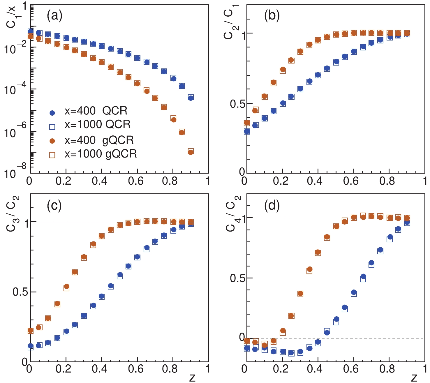
Figure 1.  (color online) Ratios of cumulants for baryon or antibaryon number as functions of quark-antiquark asymmetry z with original QCR and gQCR at two different values of total quark number x: $C_{1}/x$, $C_{2}/C_{1}$, $C_{3}/C_{2}$, and $C_{4}/C_{2}$.

with the original QCR and gQCR at two values of the total quark number $x = N_{q}+N_{\bar{q}}$. The cumulants for antibaryons are given by

Note that the first order cumulant for baryons is related to that for antibaryons by $C_{1}^{B} = C_{1}+zx/3$. As x is not small ($x\gtrsim 200$), $C_{1}/x$, $C_{2}/C_{1}$, $C_{3}/C_{2}$, and $C_{4}/C_{2}$ are almost independent of x (i.e., the system size) and are only mainly dependent on the quark-antiquark asymmetry z (proportional to the net-baryon density). Therefore, we plot their z dependence under the original and generalized QCR, respectively in Fig. 1. Panel (a) shows that fewer antibaryons are produced with gQCR than with the QCR. The antibaryon production with gQCR is more suppressed than the QCR for larger z. We can parameterize the antibaryon number [54] as $\overline{N_{\bar{B}}}/x = \left(z/3\right)\left(1-z\right)^{a}/$$\left[\left(1+z\right)^{a}-\left(1-z\right)^{a}\right]$ with $a = 3$ for QCR and $a = 5$ for gQCR. We see that the cumulant ratios $C_{2}/C_{1}$, $C_{3}/C_{2}$, and $C_{4}/C_{2}$ tend to unity at large z. This is because the antiquark number is small at large z, and the aggregation of quarks and antiquarks in phase space to form baryons and antibaryons is more stochastic and follows the Poisson distribution. Antibaryons are produced at a lower level in the gQCR, and thus the feature of the Poisson distribution is more obvious, which is reflected in the cumulant ratios in the gQCR approaching unity more quickly at large z than in the QCR. At small z, $C_{3}/C_{2}$ and $C_{4}/C_{2}$ are low and approach the Gaussian distribution.

Following the method of Refs. [35, 55], we obtain some multiplicity properties of identified hadrons by taking advantage of the stochastic combination rule. In this study, we only consider the production of octet baryons with $J^{P} = (1/2)^{+}$ and decuplet baryons with $J^{P} = (3/2)^{+}$, pseudo-scalar mesons with $J^{P} = 0^{-}$, and vector mesons $J^{P} = 1^{-}$ in the flavor SU(3) ground state. The mean values of the multiplicities for identified baryons and mesons are given by

with

where f denotes the quark or antiquark flavors in the baryon $B_{i}$, and the meson $M_{i}$, $n_{f,B_{i}}$, and $n_{f,M_{i}}$ are the number of flavor f quarks in $B_{i}$ and $M_{i}$ respectively. $S_{B_{i}}$ counts the number of different permutations in quarks and antiquarks, $g_{B_{i}}$ and $g_{M_{i}}$ are spin selection factors for $B_{i}$ and $M_{i}$, respectively. We introduce a parameter, $R_{V/P}$, to denote the relative weight of vector mesons to pseudo-scalar mesons with the same quark content, and introduce parameter $R_{D/O}$ to denote the relative weight of decuplet baryons to octet baryons with the same quark content. We assume $R_{V/P} = 0.45$ and $R_{D/O} = 0.5$ from studying hadronic yields in relativistic high-energy collisions [56, 57]. Because the values of the two parameters are extracted from the experimental data of hadronic yields, we emphasize that the two parameters can absorb the effects/contribution of various excited states and higher-mass resonances to a certain extent.

Taking the proton as an example, we have $N_{{ p}}^{\left(q\right)} =$$3N_{u}\left(N_{u}-1\right)N_{d}$ for all possible combinations of uud. Then the ratio $N_{{ p}}^{\left(q\right)}/N_{q}\left(N_{q}-1\right)\left(N_{q}-2\right)$ stands for the formation probability of the proton with the quark flavor uud. The spin selection factor for the proton is $g_{{ p}} = 1/(1+R_{D/O})$.

We introduce the configuration of multiple hadrons as $\left\{ k_{{h}_{1}}{h}_{1},\,k_{{h}_{2}}{h}_{2},\,...\right\} \equiv\left\{ k_{{h}}{h}\right\}$, where ${h}_{i}$ denotes one hadron, and $k_{{h}_{i}}$ its number in the configuration. We define the joint moment of the multiplicity for such a configuration as $N_{\left\{ k_{h}h\right\} } = \prod_{{h}_{i}}N_{{h}_{i}}^{\underline{k_{{h}_{i}}}}$, where we have used the falling factorial of the hadron multiplicity $N_{{h}}^{\underline{k_{{h}}}} = \prod_{n = 1}^{k_{{h}}}\left(N_{{h}}-n+1\right)$. The average value of the joint moment of the multiplicity reads

where $k_{B} = \sum_{{h}_{i}}k_{{h}_{i}}Q_{B,{h}_{i}}$ counts the number of baryons in the multi-hadron configuration with $Q_{B,{h}_{i}} = 1$ with ${h}_{i}$ as a baryon and $Q_{B,{h}_{i}} = 0$ for ${h}_{i}$ as a meson and an antibaryon. Similarly, $k_{\bar{B}}$ counts the number of antibaryons, and $k_{M}$ counts the number of mesons in the multi-hadron configuration. $k_{q} = \sum_{{h}_{i}}k_{{h}_{i}}Q_{q,{h}_{i}}$ counts the number of constituent quarks in the multi-hadron configuration with $Q_{q,{h}_{i}} = 3$ for ${h}_{i}$asg a baryon, $Q_{q,{h}_{i}} = 0$ for ${h}_{i}$ as an antibaryon, and $Q_{q,{h}_{i}} = 1$ for ${h}_{i}$ as a meson. Similarly, $k_{\bar{q}}$ counts the number of antiquarks. The numerator in Eq. (46) is defined as

which denotes the number of all possible combinations out of all quarks with specific flavors in the hadrons in the multi-hadron configuration, where f spans $u,d,s,\bar{u},\bar{d},\bar{s}$, and $n_{f} = \sum_{{h}_{i}}k_{{h}_{i}}n_{f,{h}_{i}}$ counts the number of f flavor quarks or antiquarks in the multi-hadron configuration.

We take a few examples of multi-hadron configurations to illustrate Eq. (46). The first example is the configuration with two protons, where we have $k_{{p}} = 2$ and $N_{{p}}^{\underline{2}}\equiv N_{{p}}\left(N_{{p}}-1\right)$, thus we obtain

where $\overline{N_{B}\left(N_{B}-1\right)}$ denotes the average for all possible baryon pairs, $N_{{pp}}^{\left(q\right)} = 3^{2}N_{u}^{\underline{4}}N_{d}^{\underline{2}}$ is the number of all possible combinations out of six quarks with specific flavors in two protons. The ratio $N_{{pp}}^{\left(q\right)}/N_{q}^{\underline{6}}$ provides the probability of the six-quark combination with a particular flavor structure $(uud)(uud)$. The second example is the configuration ${pp\bar{n}}$, we have

where the first parentheses in the second line yield the probability of two baryons with the flavor and spin structure of two protons, whereas the second parentheses yield the probability of an antibaryon with the flavor and spin structure of the antineutron.

All orders of moments and correlation functions of hadron multiplicity can be built from Eq. (46). The two-body correlation function reads

where $\alpha$, $\beta$ denote two hadrons, and we have used $\overline{N}_{\alpha\beta}\equiv\overline{N_{\alpha}N_{\beta}}$ for $\alpha\neq\beta$ and $\overline{N}_{\alpha\beta}\equiv\overline{N_{\alpha}^{\underline{2}}}$ for $\alpha = \beta$. The three-body correlation function reads

where $\overline{N_{\alpha}N_{\beta}N_{\gamma}}$ can be expressed by falling factorials,

Here we used $\overline{N}_{\alpha\beta\gamma}\equiv\overline{N_{\alpha}N_{\beta}N_{\gamma}}$ for $\alpha\neq\beta\neq\gamma$, $\overline{N}_{\alpha\beta\gamma}\equiv\overline{N_{\alpha}^{\underline{2}}N_{\gamma}}$ for $\alpha = \beta\neq\gamma$, and $\overline{N}_{\alpha\beta\gamma}\equiv\overline{N_{\alpha}^{\underline{3}}}$ for $\alpha = \beta = \gamma$. Notably, $\overline{N}_{\alpha\beta\gamma}$ is symmetric for any permutation of $\alpha$, $\beta$, and $\gamma$. The four-body correlation function can be written as

where $\overline{N_{\alpha}N_{\beta}N_{\gamma}N_{\epsilon}}$ can be expressed by falling factorials

Here, we have used $\overline{N}_{\alpha\beta\gamma\epsilon}\equiv\overline{N_{\alpha}N_{\beta}N_{\gamma}N_{\epsilon}}$ for $\alpha\neq\beta\neq\gamma\neq\epsilon$, $\overline{N}_{\alpha\beta\gamma\epsilon}\equiv\overline{N_{\alpha}^{\underline{2}}N_{\gamma}N_{\epsilon}}$ for $\alpha = \beta\neq\gamma\neq\epsilon$, $\overline{N}_{\alpha\beta\gamma\epsilon}\equiv\overline{N_{\alpha}^{\underline{3}}N_{\epsilon}}$ for $\alpha = \beta = \gamma\neq\epsilon$, and $\overline{N}_{\alpha\beta\gamma\epsilon}\equiv\overline{N_{\alpha}^{\underline{4}}}$ for $\alpha = \beta = \gamma = \epsilon$. $\overline{N}_{\alpha\beta\gamma\epsilon}$ is symmetric for any permutation of $\alpha$, $\beta$, $\gamma$ and $\epsilon$.

The cumulants of the net proton number $N_{{p}}-N_{\bar{{p}}}$ can be calculated by combinations of the above multi-body correlation functions (except $C_{1}$, which is simply the mean value of the net proton number)

In Fig. 2, we show the cumulant ratios for the net proton number with QCR and the gQCR at a given total quark number $x = 2000$ as functions of the quark-antiquark asymmetry z. We checked that the cumulant ratios of the net proton number are independent of x for large x. Here, we assume that the number of strange quarks is $N_{s} = N_{\bar{s}} = 0.45N_{\bar{u}}$, where the strangeness conservation is satisfied, and the strangeness suppression factor 0.45 is consistent with the observation in relativistic heavy-ion collisions [27]. Because the net-baryon number is fixed at given numbers of quarks and antiquarks, Fig. 2 only shows the fluctuations of the net proton number brought by the quark combination process. $C_{1}/C_{2}$ and $C_{3}/C_{2}$ of the net proton number increase with z and approach to 1.5 and $1/3$ as $z\to1$, respectively. $C_{4}/C_{2}$ decreases with z and approaches $-1/3$ as $z\to1$. These results differ from those of the statistical model for hadron resonance gas with thermal equilibrium [58], in which $C_{1}/C_{2}$ and $C_{3}/C_{2}$ increase to one, and $C_{4}/C_{2}$ almost keeps a constant of one at large baryon number chemical potential.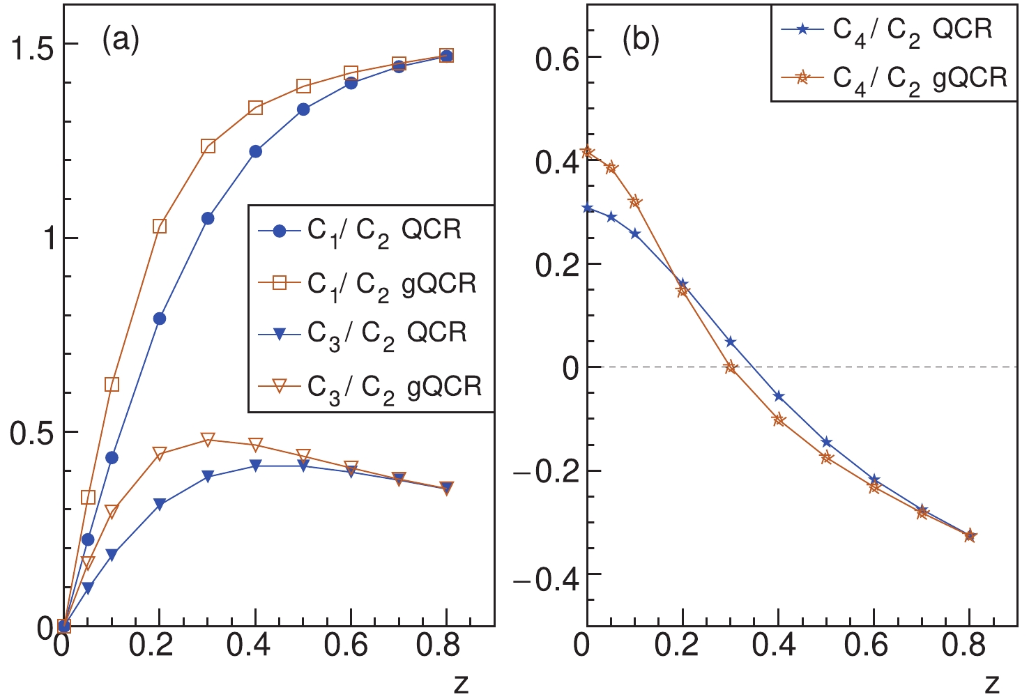

Figure 2.  (color online) Cumulant ratios of net proton number directly produced through QCR and gQCR as functions of quark-antiquark asymmetry z at x = 2000.

The numbers of quarks and antiquarks may fluctuate in high-energy collisions event by event, such that hadronic observables should be influenced by fluctuations at the quark level. We denote the distribution of quark numbers at hadronization as

and the event average of a hadronic observable $A_{{h}}$ is given by

where $\overline{A}_{{h}}\left(\{N_{f}\}\right)$ denote the average at fixed quark and antiquark numbers, obtained in the previous section.

In the practical evaluation, it is more convenient to take the expansion of $\overline{A}_{{h}}\left(\{N_{f}\}\right)$ in $N_{f}$ around the event-average numbers of quarks and antiquarks $\{\langle N_{f}\rangle\}$ as

where $\delta N_{f} = N_{f}-\langle N_{f}\rangle$ and the subscript '0' denotes the values at $\langle N_{f}\rangle$. Substituting into Eq. (57), we obtain

which involves multi-body correlations for the quark and antiquark number with the quark number distribution $P\left(\{N_{f}\}\right)$

where we used the same symbols C as in Sec. 5 to denote the quark number correlation functions, but with quark flavor indices.

Using the above moment expansion method, we can study, for the selected phase-space window such as the midrapidity region $|y|<0.5$, the influence of different quark and antiquark distributions in the window on the production of hadrons at hadronization. This extends the applicability of QCR described in Sec. 2 and 3, where only the stochastic quark-antiquark population is considered.

The long life (stable) hadrons measured in experiments include contributions from resonance decays. In this section, we consider the influence of resonance decays on multiplicity correlations of long-life hadrons. For a resonance ${h}_{i}$, the hardons' stable daughters are denoted as $\alpha , \; \beta , \gamma$, etc., and the corresponding decay branching ratios are $D_{i\alpha}$, $D_{i\beta}$, $D_{i\gamma}$, etc., respectively. The distribution function of $\left\{ N_{\alpha},N_{\beta},N_{\gamma},\cdots\right\}$ from decays of the resonance ${h}_{i}$ with the particle number $N_{{h}_{i}}$ is denoted as $f\left(N_{{h}_{i}},\left\{ N_{\alpha}^{i}\right\} \right)$, where $N_{\alpha}^{i}$ denotes number of the stable hadron $\alpha$ from the resonance ${h}_{i}$. We take the multi-nominal distribution for the selection of decay channels. Convoluting with the joint distribution of directly produced hadrons $P\left(\left\{ N_{{h}_{i}}\right\} ,\left\{ \left\langle N_{f}\right\rangle \right\} \right)$ at hadronization, we obtain joint distributions of stable hadrons $F\left(\left\{ N_{\alpha},N_{\beta},N_{\gamma},\cdots\right\} \right)$ [35].

From the joint distribution functions of stable hadrons, we obtain the average yield of a stable hadron $\alpha$

where the index i runs over all directly produced hadron species, including stable hadrons (we define $D_{\alpha\alpha} = 1$), and we use the shorthand notation $N_{i}\equiv N_{{h}_{i}}$. The two-body multiplicity correlation function is

The three-body multiplicity correlation function of stable hadrons is

The four-body multiplicity correlation function of stable hadrons is

The higher order multiplicity correlation functions can similarly be derived from the joint distribution functions of stable hadrons.

In this section, we take the simple example of a quark system and calculate the cumulant ratios for net protons in the final state with gQCR. We discuss our results in the context of the experimental observation in Au+Au collisions at RHIC.

We consider a quark system with the property $S\sigma\equiv C_{3}/C_{2} = z$ and $\kappa\sigma^{2}\equiv C_{4}/C_{2} = 1$ for the baryon quantum number, which is similar to the base line of the grand canonical ensemble in the statistical model [59]. A simple case for the quark number correlation functions satisfying the above property is

for diagonal elements and non-vanishing off-diagonal elements ($f_{1}\neq f_{2}$)

We assume the following properties for correlation functions of the strangeness as a result of the strangeness conservation

Because the total quark number x in the mid-rapidity region $|y|<0.5$ in central heavy-ion collisions at RHIC energy is usually large ($x\gtrsim$500), the cumulant ratios for net protons in the final state in our model is not sensitive to x (the system size). Here, we just take $x = 5000$ in the calculation. We use Eq. (61) to fit the data of the $\bar{{p}}/{p}$ yield ratio in Au+Au collisions and determine z in the collision energy range $\sqrt{s_{NN}}\in[7,200]$ GeV.

In Fig. 3, we show the results for the cumulant ratios for net protons in the final state at different collisional energies. Our results only incorporate the contributions of quark number fluctuations and correlations up to the fourth order, as in Eq. (59). The auxiliary horizontal axis shows the corresponding quark-antiquark asymmetry parameter z. Results including the contributions from strong and electromagnetic (S&EM) decays of resonances are depicted by dashed lines, while results with full decay contributions including weak decays are depicted by solid lines. The STAR data are shown in solid circles with error bars.

Figure 3.  (color online) Cumulant ratios for net protons at different collision energies. Solid circles with error bars depict experimental data [43, 60]. Solid and dashed lines represent theoretical results of SDQCM.

In the figure, we see that the cumulant ratios for net protons as functions of collisional energies in our model describe the experimental data: $M/\sigma^{2}$ and $S\sigma$ increase with z or equivalently decrease with collisional energies, while $\kappa\sigma^{2}$ decreases with collisional energies until it reaches a minimum at $\sqrt{s_{NN}} =$20 GeV and then increases toward unity at high energies. Our results for $\kappa\sigma^{2}$ are the consequence of the competition between two effects: (1) The cumulant ratio $C_{4}/C_{2}$ from directly produced net protons by quark combinations, as shown in Fig. 2, always decreases with increasing z; (2) The cumulant ratio $C_{4}/C_{2}$ for baryons or antibaryons, as shown in Fig. 1, rapidly increases as $z\!\!\gtrsim\!\!0.2$ (corresponding to $\sqrt{s_{NN}}\!\!\lesssim\!\!20$ GeV).

We now provide some remarks regarding the results for $\kappa\sigma^{2}$ of net protons. Although our results for net protons can reproduce the nontrivial dependence on collisional energies, we always have $\kappa\sigma^{2} = 1$ for net baryons at all collisional energies because of the flavor/charge conservation in the quark combination. Therefore, our results indicate that cumulant ratios of the net proton number in this simple case do not exactly follow those of the net baryon number. This is different from the statistical model [57] for hadron resonance gas with thermal equilibrium, which predicts similar cumulant ratios for net-protons and net-baryons.

We emphasize that the current results are preliminary and are mainly used to show the potential application of our model in hadronic fluctuations, and the related phase transition in relativistic heavy-ion collisions. Some limitations in current calculations should be clarified. In this study, we only consider the production of ground-state hadrons. Effects of higher-mass resonances are only partially absorbed by parameters $R_{V/P}$ and $R_{D/O}$. According to our previous study [35], the production of hadrons with small yields tends to follow the Poisson distribution. Including those higher-mass resonances with small yields may enlarge the fourth moments of protons to a certain extent. Our model is a static one and does not consider the diffusion of hadrons/quarks during the finite hadronization time, which will have some influence on the calculation of net-proton fluctuations in a specific window. Further, to make final comparison with the data of net protons, we should consider more realistic quark number fluctuations and correlations in the studied rapidity window, which may be obtained by grand-canonical statistics of the thermal quark system or by canonical statistics with a Bernoulli trial selection of the specific window. We should also consider other effects related to the finite acceptance window, such as the diffusion/blur of charges during the hadronic scatterings stage as well as that caused by resonance decay [55, 58, 61–73]. We will study these effects in this framework in the future.

We developed a new statistical method to solve the probability distribution for the number of baryons, antibaryons, and mesons formed in the hadronization of a constituent quark and antiquark system governed by the quark combination rule (QCR) in the quark combination model developed by the Shandong Group. We use a set of numbers $(N_{M},N_{B},N_{\bar{B}},N_{r},N_{\bar{r}})$ to classify the outcome of implementing the QCR for a queue of $N_{q}$ quarks and $N_{\bar{q}}$ antiquarks, where there are $N_{M}$ mesons, $N_{B}$ baryons, and $N_{\bar{B}}$ antibaryons formed by combination but with $N_{r}$ quarks and $N_{\bar{r}}$ antiquarks left without forming hadrons. The number of different ways of a given configuration $(N_{M},N_{B},N_{\bar{B}},N_{r},N_{\bar{r}})$ is denoted as $F(N_{M},N_{B},N_{\bar{B}},N_{r},N_{\bar{r}})$. We build the recursive relation for $F(N_{M},N_{B},N_{\bar{B}},0,0)$. We adopt the generating function method to solve the recursive relation and provide the analytical expression of $F(N_{M},N_{B},N_{\bar{B}},0,0)$. This method is far simpler than the previous one and is easy to generalize. To accommodate the baryon yield in experimental data in relativistic heavy-ion collisions, we consider a generalized combination rule (gQCR). We provide the solution of the baryon and meson probability distribution function under the new rule. Because the (anti)baryon production is more suppressed in the gQCR, we find that the cumulant ratios of the antibaryon number achieve Poisson statistics more rapidly in the gQCR than in the QCR with increasing baryon number density.

We studied the multiplicity fluctuation and correlation functions for identified baryons directly produced in collisions. We also studied correlation functions of final state hadrons including contributions from resonance decays. As an illustrative example, we consider a quark-antiquark system with the property $S\sigma = z$ and $\kappa\sigma^{2} = 1$ for the baryon quantum number, which is similar to the base line in the grand-canonical ensemble in the statistical model. We calculate the cumulant ratios in the quark combination model and find that $S\sigma$ for net protons in the model increases with decreasing collisional energies, which is consistent with the experimental observation. More interesting is that $\kappa\sigma^{2}$ for net protons has a nontrivial energy behavior consistent with the data.

We dedicate this work to Qu-bing Xie (1935-2013) who was the teacher, mentor and friend of ZTL, FLS, and QW.

We present two properties for $F(N_{M},N_{B},N_{\bar{B}},N_{r},N_{\bar{r}})$ in this appendix.

Property 1. For $(N_{r},N_{\bar{r}}) = (1,0),(0,1)$, $F(N_{M},N_{B},N_{\bar{B}},N_{r},N_{\bar{r}})$ can be expressed in terms of $F(N_{M}^{\prime},N_{B}^{\prime},N_{\bar{B}}^{\prime},0,0)$ with $N_{M}^{\prime}\leqslant N_{M}$, $N_{B}^{\prime}\leqslant N_{B}$ and $N_{\bar{B}}^{\prime}\leqslant N_{\bar{B}}$,

where the coefficients $C_{n_{B},n_{\bar{B}}}^{10}(n_{M})$ are given by $C_{0,0}^{10}(n_{M}) = 1$ and

for $a+b>0$. The coefficients $C_{n_{B},n_{\bar{B}}}^{01}(n_{M})$ are given by $C_{0,0}^{01}(n_{M}) = 1$ and

for $a+b>0$. The sums over $n_{B}$, $n_{\bar{B}}$, and $n_{M}$ in Eq. (A1) continue until any of the baryon, antibaryon, or meson number become negative, since $F(N_{M},N_{B},N_{\bar{B}},N_{r},N_{\bar{r}}) = 0$ for the case where any of $N_{M}$, $N_{B}$, $N_{\bar{B}}$, $N_{r}$, or $N_{\bar{r}}$ are negative.

Property 2. For $(N_{r},N_{\bar{r}}) = (2,0),(0,2)$, $F(N_{M},N_{B},N_{\bar{B}},N_{r},N_{\bar{r}})$ can be expressed in terms of $F(N_{M}^{\prime},N_{B}^{\prime},N_{\bar{B}}^{\prime},0,0)$ with $N_{M}^{\prime}\leqslant N_{M}$, $N_{B}^{\prime}\leqslant N_{B}$ and $N_{\bar{B}}^{\prime}\leqslant N_{\bar{B}}$,

where the coefficients are identical to Eqs. (A2, A3): $C_{n_{B},n_{\bar{B}}}^{20}(n_{M}) = C_{n_{B},n_{\bar{B}}}^{10}(n_{M})$ and $C_{n_{B},n_{\bar{B}}}^{02}(n_{M}) = C_{n_{B},n_{\bar{B}}}^{01}(n_{M})$.

To demonstrate the two properties in Eq. (A1) and Eq. (A4), we can solve $F(N_{M},N_{B},N_{\bar{B}},2,0)$ by substituting the first equation into the third one in Eq. (31),

In the same manner, we can solve $F(N_{M},N_{B},N_{\bar{B}},0,2)$ by substituting the second equation into the fourth one in Eq. (31)

From Eqs. (A5, A6) we obtain Eq. (A4). Then from Eq. (A4) and the last two equations of Eq. (31) we obtain Eq. (A1).

We derive the recursive equation for $F(N_{M},N_{B},N_{\bar{B}},0,0)$ with the help of Eq. (31). We start from Eq. (7), which also holds for gQCR. Using Eq. (31), Eq. (7) can be rewritten as

where G is defined by

We need to define another auxiliary function

where we used the first two equalities of Eq. (31) to obtain second line and used Eq. (B1) to obtain the last line. In contrast, we can also derive another form of $H(N_{M},N_{B},N_{\bar{B}})$ by applying the last two equalities and subsequently the first two equalities of Eq. (B3) and finally applying Eq. (31). The result is as follows:

From Eq. (B3), we also obtain

By setting Eq. (B4) equal to Eq. (B5), we derive the recursive equation for G and then for $F(N_{M},N_{B},N_{\bar{B}},0,0)$ through Eq. (B1), as in Eq. (32).

We multiply Eq. (32) by $x^{N_{M}}$ and sum over $N_{M}\geqslant3$ (the equation is well defined for $N_{M}\geqslant3$). Hence, we obtain

One can verify that a complete cancellation occurs for terms proportional to $x^{2}$ and those proportional to x after applying Eq. (32) for $N_{M} = 2$ and $N_{M} = 1$, respectively. The constant terms in F read

where we used the initial value $F(0,N_{B},N_{\bar{B}},0,0) = \delta_{N_{B}N_{\bar{B}},0}$. This means that if there are no mesons, baryons and antibaryons cannot co-exist, and if there are only quarks or antiquarks in the system, the number of different queues is 1. Then, Eq. (C1) is simplified as

We now multiply Eq. (C3) by $y^{N_{B}}z^{N_{\bar{B}}}$ and take a sum over $N_{B}\geqslant1$ and $N_{\bar{B}}\geqslant1$ to obtain

To simplify the above equation, we use

and

as well as Eqs. (36) and (37), we finally obtain Eq. (38).

From Eq. (38) we can extract $F(N_{M},N_{B},N_{\bar{B}},0,0)$, the coefficient of $x^{N_{M}}y^{N_{B}}z^{N_{\bar{B}}}$ in the polynomial expansion of $A(x,y,z)$. To this end, we rewrite $A(x,y,z)$ as

where we used the multinomial theorem

with multinomial coefficients

Then, we can extract the coefficient of $y^{N_{B}}z^{N_{\bar{B}}}$ as

where $C_{1,2,3,4}$ are given by

We have expressed the summation indices j and k in terms of $N_{B}$ and $N_{\bar{B}}$ for a given summation index i. The sum over i involves a finite number of terms. For example, in $C_{1}$, we have $N_{B}+N_{\bar{B}}\geqslant i\geqslant{\rm Max}(N_{B},N_{\bar{B}})$, since any term in the summation with the factorial of a negative integer in the denominator is vanishing.

We can factorize the following two polynomials as

and expand $C_{1}$, $C_{2}$, $C_{3}$, $C_{4}$ into a power series of x with the help of the binomial theorem. Then, we can extract the coefficient of $x^{N_{M}}$ in $C(y^{N_{B}}z^{N_{\bar{B}}})$. This yields the coefficient of $x^{N_{M}}y^{N_{B}}z^{N_{\bar{B}}}$ in $A(x,y,z)$ or $F(N_{M},N_{B},N_{\bar{B}},0,0)$ as the sum of the following four terms

which yield the final result of gQCR in Sec. 3.