The first excited single-proton resonance in ¹⁵F by complex-scaled Green's function method

The new generation radioactive ion beam facilities enabled the discovery of numerous exotic phenomena near the drip line, such as proton halo [1, 2], neutron halo [3-6], changes of nuclear magicity [7, 8], etc. Considering that the Fermi surface for exotic nuclei is very close to the continuum, the valence nucleons are easily scattered into the continuum. The contribution of the continuum, especially the resonance in the continuum, is particularly important. With the small Coulomb barriers, some of resonances are oriented to be very broad and the ground state (g.s.) of ¹⁵F is viewed as a (broad) s-wave resonance [9-11]. However, the first excited state (5/2⁺) of the unstable ¹⁵F is viewed as a narrow resonance with higher Coulomb barriers. Because the Coulomb barrier holds the proton for a long time, the 5/2⁺ state is very narrow [12]. Moreover, another important feature of ¹⁵F is a new resonant state 1/2⁻, which was investigated by the Gamow Shell Model [13]. The very narrow width (36 keV) was pointed out for the first time with high precision. Further steps to explore exotic phenomena in ¹⁵F will be quite interesting.

During the past decades, the proton-rich nuclei became accessible in the proton elastic resonance scattering reaction [14]. Various experiments on the resonances in ¹⁵F are in progress. The ²⁰Ne (³He, ⁸Li) reaction had been used to investigate the unstable nucleus ¹⁵F in 1978 [15] and 0.24(3) MeV (the first excited state 5/2⁺) is close to the value indicated in the analysis ($ \Gamma\approx 0.2 $ MeV of 5/2⁺) of Ref. [16] and our predictions ($ E_r = 2.770 $ MeV and the width $ \Gamma = 0.239 $ MeV) for the resonant state $ 1d_{5/2} $. Moreover, the radioactive beams of ¹⁴O were usually utilized to populate the resonant states (1/2⁺, 5/2⁺) in ¹⁵F [17, 18], where the peaks in the curve, that differential cross sections plotted as a function of the scattering angle, are used to present the resonant states.

Considering the dominant role of the resonant states in thw proton drip line, numerous methods were developed for probing single particle resonances. The developed multi-channel algebraic scattering (MCAS) theory [12] is highly appropriate for narrow resonances. Based on the MCAS theory, three negative parity states (1/2⁻, 5/2⁻, 3/2⁻) in ¹⁵F with the widths of only a few keV were found by Canton et al. [12]. Fortune and Sherr were committed to studying the ground and excited states of ¹⁵F for decades, by investigation with a potential model [19-21]. The R-matrix theory is usually used in elastic scattering experiments to analyze low-lying resonances [22], where the two lowest resonant states (1/2⁺ and 5/2⁺) in ¹⁵F were fitted by the R-matrix. The R-matrix theory can also be used to determine spectroscopic properties of the states [23]. The Gamow Shell Model (GCM) is likewise an efficient tool for exploring single-particle resonant states in the proton drip line [13], where the GCM provides relatively narrow resonances with high excitation energies of ¹⁵F. Meanwhile, several bound-state-like methods were developed for the single-particle resonant states. These include the S-matrix [24], analytic continuation in the coupling constant (ACCC) [25], complex scaling method (CSM) [26], the Green's function method [27], etc.

Although many experiments and theoretical studies [17, 20, 24] are devoted to the investigations for ¹⁵F, the width of the 5/2⁺ still has large uncertainty. In rare cases, the proton resonant state is extremely narrow at higher energies, even for the resonance with low angular momentum. ¹⁵F sets such an example in this study. Since Fortune's predictions in Ref. [16] and the single-neutron resonant states can be successfully located by the complex-scaled Green's function method (CGF) [28-32], here we use the CGF method to extend the investigation of single-proton resonant states with the solution of the Schrödinger equation, especially for the ground and first-excited states. The choice of ¹⁴O as the core of ¹⁵F is mainly attributed to two reasons. One is that the strong neutron shell closure effect also happens in ¹⁴O [33], the other is that Z = 8 (magic number) plus one proton could be better to investigate the single particle resonant states in neutron-deficient nuclei. The paper is constructed as follows: the general formalism of the CGF method is presented in Sec. 2; Sec. 3 presents the numerical details and results. Finally, the main conclusions are summarized in Sec. 4.

To explore the single-proton resonances in ¹⁵F, we first sketch the theoretical formalism. The Hamiltonian of this system is written as

where the potential consists of the following four parts

and the spin-orbit coupling potential

Here, $ f(r) = \dfrac{1}{{1+\exp (\frac{{r-R}}{a})}} $, $ k(r) = r\dfrac{{\rm d}f(r)}{{\rm d}r} $. The parameter $ m_{\pi } $ is fixed at 135 MeV in Ref. [24] to investigate ¹⁵F. Because the Coulomb interaction potential is widely used in nuclear physics, the deformed Coulomb potential is given by

here $ \alpha $ is the fine-structure constant. The Hamiltonian H and wave function $ \psi $ are transformed as

Here, $ U(\theta ) $ is a complex rotation operator defined by the transformation $ \vec{r}\rightarrow \vec{r}{{\rm e}^{{\rm i}\theta }} $, and $ H_{\theta }(\psi _{\theta }) $ is the complex scaled Hamiltonian (wave function) with the complex rotation angle $ {\theta } $ in Refs. [34-36]. The corresponding complex scaled equation becomes

By solving the complex scaled Eq. (8), we can single out bound states and resonant states. Details are provided in the literature [29]. However, there are some disadvantages in CSM that are indicated in Ref. [31]. For example, to accurately determine resonance parameters, we need to repeat diagonalization of the Hamiltonian in complex scaling calculations, while a complicated loop integral is imposed on the Green's function method in search of resonant states. Therefore, the CSM is combined with the Green's function method by defining the complex-scaled Green's function (CGF) as

in the coordinate representation

Then, with an extended completeness relation

the density of states can be defined as

Employing the basis expansion method, the density of states can be approximately expressed as

In Eq. (12), $ {\psi _{b}^{\theta }} $ and $ {\psi _{r}^{\theta }} $ are the complex scaled wave functions for the bound and resonant states, respectively, while $ {\psi _{c}^{\theta }} $ is the wave function of the rotated continuum. The bra states with tilde represent the bi-orthogonal counterparts of the ket states. Detailed explanations can be found in Ref. [37]. In Eq. (12), $ {E_{b}},{{E_{r}^{\theta }}} $, and $ {{E_{c}^{\theta }}} $ represent the energy eigenvalues of $ {H_{\theta }} $ for the bound states, resonant states, and rotated continuum, respectively. $ {N_{b}} $ and $ N_{r} $ are the numbers of bound and resonant states, respectively. In Eq. (13), N represents the total number of states (the size of basis). Because of the normalization of the wave functions for bound and resonant states, the integration on $ {\vec{r}} $ in Eq. (12) is unity. However, for the continuum, there appears singularity in the integration $ {\vec{r}} $, which can be eliminated using the basis expansion method in the discretization of the energy spectrum. Then, the density of states can be expressed by the bound state energies $ {E_{b}}(b = 1,2,...,{N_{b}}) $, the resonance complex energies $ E_{r}^{\theta } = {E_{r}}-{\rm i}\Gamma _{r}/2(r = 1,2,...,{N_{r}}) $, and rotated continuum energies $ \varepsilon _{c}^{\theta } = \varepsilon _{c}^{R}-{\rm i}\varepsilon _{c}^{I}\left( c = 1,2,...,N-N_{b}-N_{r}\right) $.

As there are approximations in realistic calculations, $ \rho _{\theta }^{N}(E) $ is slightly dependent on $ \theta $. The dependence can be weakened by subtracting the background of $ H_{\theta } $, which is defined as the density of continuum states $ \rho _{\theta }^{0N}(E) $:

where $ \varepsilon _{k}^{0}(\theta ) = \varepsilon _{k}^{0R}-{\rm i}\varepsilon _{k}^{0I} $ are the eigenvalues of the asymptotic Hamiltonian $ H_{\theta }^{0} $ in the form of $ {H_{\theta }} $ with $ r\rightarrow \infty $. After subtracting the background of $ H_{\theta } $, the continuum level density (CLD) $ \Delta \rho (E) $ is as the difference between the density of states $ \rho _{\theta }^{N}(E) $ and the density of continuum states $ \rho _{\theta }^{0N}(E) $:

The CLD is also related to the scattering phase shift $ \delta (E) $,

By performing integration of every term, the phase shift $ \delta (E) $ is obtained as:

With the definitions of $ \delta _{r} $, $ \delta _{c} $, and $ \delta _{k} $

the phase shift is then expressed as

Based on the relationship between the phase shift and the cross section, the partial cross section for spherical nuclei is expressed as

where $ k^{2} = 2E\mu/\hbar ^{2} $ with the reduced mass $ \mu $.

We explore the single-proton resonance in ¹⁵F using the formalism represented above. Based on the experiment and data analysis with the R-matrix, the model parameters are determined by reproducing the experimental single-proton separation energy $ {S_p} = -1.51 $ MeV, suggested in Ref. [17]. The single-particle energy $ \varepsilon $ of the last valence proton is determined from the $ {S_p} $ energy, $ \varepsilon = -{S_p} $. Then, the $ 1/2^{+} $ (g.s.) resonance energy of ¹⁵F was determined to the one-proton decay energy 1.51 MeV, which correspond to the single-proton separation energy. For the broad resonance $ 1/2^{+} $ with $ \Gamma\approx0.84-1.2 $ MeV [17, 38], the obtained width is 1.07 MeV using our method. These calculations confirm that the parameters are suitable for the following discussion. Under such circumstances, the potential geometry is fixed. For the central potential, $ V_{0} = 53.40 $ MeV, $ a = 0.64 $ fm, and $ r_{0} = 1.17 $ fm for the radius $ R = r_{0}A^{1/3} $. For the spin-orbit potential, the strength of the spin-orbit coupling $ V_{0}^{sl} = 7.46 $ MeV is applied. Moreover, the Coulomb potential with a radius $ R_c = R $ is assumed. The complex-scaled equation is solved by expansion in Laguerre polynomials. When the basis is truncated up to 100 shells, the size of all concerned subspaces is sufficiently large to study the single-proton resonant states in present calculations. With the fitted parameters, the pattern is similar to the neutron resonant states [39] in the following calculations. Fig. 1 shows the change of the eigenvalues of $ H_{\theta} $ with $ \theta $ from $ 3^{\circ } $ to $ 7^{\circ } $ by a step of $ 1^{\circ } $. The resonant states are clearly isolated from the continuum with increase in the rotation angle. Possibly, the positions of the resonant state $ 5/2^{+} $ hardly change with increasing $ \theta $, however the real situation does not conform to this situation. More details are given in Fig. 2.

Figure 1.  (color online) Variation of eigenvalues of $ H_{ \theta} $ with $ \theta $ for the $ 1d_{5/2} $ state, where the complex-scaling parameter $ \theta $ varies from $ {3^\circ } $ to $ {7^\circ } $ by steps of $ {1^\circ }. $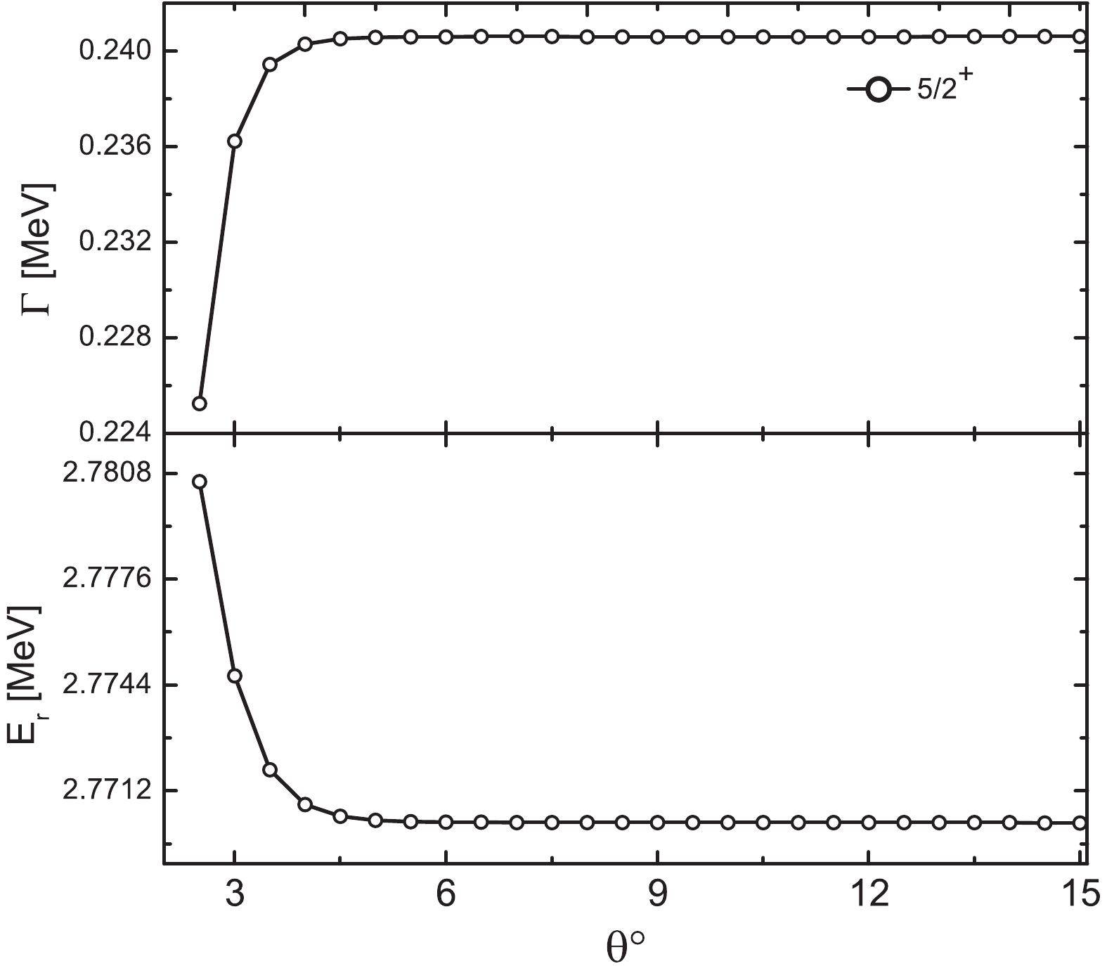

Figure 2.  $ \theta $ trajectory for resonant state $ 1d_{5/2}. $

Although the resonant states are separated from the continuum, we still need to determine the most appropriate $ \theta $ value for the investigation of the resonances in our calculations in Fig. 2, where the $ \theta $ trajectory is plotted. Extending the ABC-theorem [34-36] in realistic calculations, the condition that the resonance parameters are independent on $ \theta $ ($ \frac{{\rm d} E_{\theta}}{{\rm d} \theta} = 0 $) is not available. A common approach is considering that the obtained values for the resonance parameters depend slightly on $ \theta $ by a finite basis expansion in Ref. [40]. Hence, the best estimate for the proton resonance parameters is $ \left|\frac{{\rm d} E_{\theta}}{{\rm d} \theta}\right| $ at the minimal value. When $ \theta $ is small (less than $ 6^{\circ } $), the resonance position is very sensitive to the complex rotation angles. Once $ \theta $ is larger than $ 6^{\circ } $, the energies and widths of resonant states are almost independent of $ \theta $. As long as the complex rotation angle $ \theta $ is sufficiently large, the obtained energies and widths are reliable. However, it is worth noting that $ \theta $ is not infinite with a Woods–Saxon-type potential in the present work, and the effective range is $0<\theta<\tan ^{-1} $$ (\pi a / R) $. Hence, $ \theta = 6^{\circ } $ as an optimal value is adopted in the following. Moreover, the corresponding width and energy are 0.240 MeV, 2.770 MeV, respectively, for the resonant state $ 1d_{5/2} $ with CSM, respectively.

Comparing with the the resonance energies and widths by CSM, we apply the complex-scaled Green's function method to calculate the continuum level density to determine the optimal resonance locations. The results are exhibited in Fig. 3. Employing the same technique as in Ref. [32], the available energy is obtained at $ E_r = 2.770 $ MeV and the width $ \Gamma = 0.239 $ MeV for the resonant state $ 1d_{5/2} $. These calculation results are close to the experimental value 0.24(3) MeV in Ref. [15], which is the first value close to Fortune's analysis (0.2 MeV) in Ref. [16]. By examining the spectroscopic factor, Fortune pointed out a serious problem that the width with 0.3 MeV obtained from Refs. [12,13,18] is too large compared with the one expected from spectroscopic factors for the lowest $ 5/2^{+} $ state in other A=15 nuclei. However, the current obtained width is 0.240 MeV with the CSM and 0.239 MeV with CGF. Hence, our calculations are closer to the width obtained by Fortune than previous results, and further details are provided in Table 1, which confirms that our method is reliable in determining the width of the resonance. At the same footing, we obtained the resonance energy 2.770 MeV, which is close to the average value (2.794 MeV) obtained by the previous method in Ref. [16]. It is further confirmed that the complex-scaled Green's function method hold the advantages for the study of single-particle resonant states near the drip line.

$J^\pi$	$E_p$ /MeV	$\Gamma$ /MeV	Ref.
$1/2^{+}$(exp)	$1.51\pm 0.11$	1.2	[17]
	1.56(13)	$0.6(+0.8/-0.4)$	[10]
	1.31(1)	0.853(146)	[18]
	1.270(10)(10)	0.376(70)	[13]
(calc)	1.31	0.8	[12]
	1.39-1.51	$\sim0.8$	[20]
	1.194	0.531	[24]
	1.51	1.07	CGF
$5/2^{+}$(exp)	2.78(1)	0.311(10)	[18]
	$2.853\pm 0.045$	0.34	[17]
	2.763(9)(10)	0.305(9)(10)	[13]
	2.67(10)	0.5(2)	[11]
(calc)	2.785	$\sim0.2$	[16]
	2.78	0.3	[12]
	2.780	0.293	[24]
	2.770	0.239	CGF

Table 1.  Energies and widths calculated for ¹⁵F states with $ J^{\pi} = 1/2^{+} $ and $ 5/2^{+}. $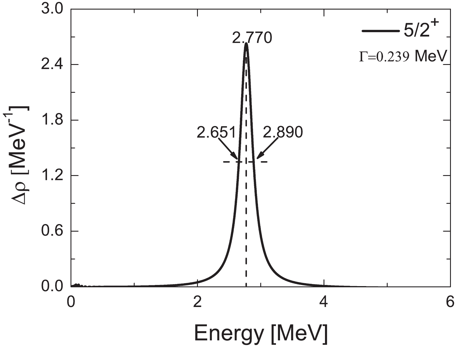

Figure 3.  The continuum level density $ \Delta \rho (E) $ for the $ 1d_{5/2} $ state with the complex-scaling parameter $ \theta = 6^{\circ }. $

To make the results reliable, the phase shift method (or $ \delta = \pi/2 $ rule) will provide a check for studying the single-particle resonant states [24]. The phase shift $ \delta $ of the first excited state $ 1d_{5/2} $ is shown in Fig. 4 with $ \theta = 6^{\circ } $. The first excited state can be regarded as a ¹⁴O core plus a proton in the $ 1d_{5/2} $ orbit, which is viewed as a single-particle state in the system (¹⁵F = ¹⁴O+p). The resonant energy (one-proton decay) $ E_r = 2.789 $ MeV can be obtained from passing through $ \delta = \frac{\pi}{2} $, which yields values that are very close to the CGF and other theories [16, 41]. In this study, we converted the obtained phase shifts into resonance cross sections using Eq. (20), which is plotted in Fig. 5. The resonance energy is determined by the cross section $ \sigma $ reaching its maximum value. Hence, the sharp peak value at $ E = 2.787 $ MeV is considered to be the $ 1d_{5/2} $ resonance energy. The energy obtained is likewise in agreement with the results of CSM and CGF.

Figure 4.  ¹⁴O+p scattering phase shift for the $ 1d_{5/2} $ state of ¹⁵F generated by the Woods-Saxon potential. Remaining parameters are same as those in Fig. 3.

Figure 5.  The cross section of $ l = 2 $ partial wave in ¹⁵F. Remaining parameters are same as those in Fig. 3.

Table 1 lists the results for the energies and widths of the low-lying states for ¹⁵F, which are then compared to each other. The ground state in ¹⁵F is a broad resonance, except for the value 0.376(70), and the narrower width is also supported by some theoretical predictions [42]. Our calculations 1.07 MeV (width) observed as a broad wave belong to $ \Gamma\approx 0.531-1.2 $ MeV in Table 1, and 1.51 MeV is also in the energy range. For the $ 1d_{5/2} $ state, the width is as small as 0.239 MeV, which also belongs within the range (0.2–0.5 MeV) in Table 1. The suggested value 0.20 MeV by Fortune is slightly smaller than our results. This indicates the calculations by the CGF method are reliable.

To further examine the applicability and validity of the current model, we explore the dependence of the resonant parameters on the shape of the potential. Using Woods-Saxon potential for the low-lying states for $ ^{15} $F, there are three parameters, namely depth of potential $ V_0 $, surface diffuseness a, radius parameter $ r_{0} $. Keeping $ V_{0} = 53.40 $ MeV and the radius $ r_{0} = 1.17 $ fm fixed, we vary the parameter a to investigate how the energies and widths of the $ 2s_{1/2} $ and $ 1d_{5/2} $ states are sensitive to surface diffuseness a in Fig. 6. With the increase of a, the energies and widths of the resonant states decrease, which is expected because the potential becomes more dispersed. With the lower resonance energies and narrower resonance widths, the lifetime of single proton states would become longer with increasing a.

Figure 6.  (color online) Parameters are same as Fig. 3, green circles represent resonant states with $ a = 0.64 $ fm, $ r_{0} = 1.17 $ fm, $ V_{0} = 53.40 $ MeV.

A similar trend is observed when we vary the central depths $ V_0 $, keeping other parameters fixed. The results are displayed in the middle panel of Fig. 6. With the deeper potential, the energies and the widths of the $ 2s_{1/2} $ and $ 1d_{5/2} $ states both decrease. Compared with the $ 2s_{1/2} $ state, the energy of the $ 1d_{5/2} $ state drop faster, and there appears to be a crossover in the resonance energy with deeper potential. When the potential further deepens past 59 MeV, the resonant states show a disappearing trend, and the width would hence be too narrow. The lifetime of the resonant states is a reciprocal of the width, hence if one state has a narrower width, it would indicate that it is more stable. Because the depth of potential significantly influences the stability of resonant states, the relationship between the depth of potential and the resonant states can present the evolution of levels from unstable to stable nuclei.

As $ r_0 $ is particularly important for comparing resonant states of different isotopes, the influence of $ r_0 $ on the resonance is shown in the right panel of Fig. 6. With increasing $ r_0 $, the energies and widths of resonant states also decrease. The two states are degenerated around $ r = 1.23 $ fm. The resonance energies become lower, and the resonance widths become narrower. This can be explained in terms of the increased $ r_0 $. The potential becomes broader, which causes falling of the levels. Further increasing $ r_0 $, the resonant states are likely to become the weakly bound states. The phenomena is in accordance with the effect of a and $ V_0 $ on resonant states. This conclusion is useful to recognize the level structure beyond the drip line.

From Fig. 6, we see that $ 2s_{1/2} $ level is lower than $ 1d_{5/2} $ level for ¹⁵F. Compared with the traditional shell structure in stable nuclei, these two states are inverted, which may occur in the exotic nucleus [43, 44]. It is worth to mention that ¹⁵C and ¹⁵F are mirror nuclei, and for ¹⁵C [4], the $ 2s_{1/2} $ orbit is likewise below the $ 1d_{5/2} $ orbital, which induces the one-neutron halo. Hence, the one-proton halo of ¹⁵F may occur. Among the parameters $ a, V_{0}, r_{0} $, the energies and widths are less sensitive to the surface diffuseness a. Thus, it is inappropriate to obtain the energy of single-proton resonance by increasing a. With the increasing $ V_{0}, r_{0} $, the energy of $ 1d_{5/2} $ state drops faster than that of the $ 2s_{1/2} $ state, which indicates if the resonant state $ 2s_{1/2} $ becomes a weakly bound state, the $ 1d_{5/2} $ orbit will be lower than $ 2s_{1/2} $ orbit, and the inversion of sd states is broken. Different from ¹⁵C, it is difficult to form one-proton halo for ¹⁵F in the spherical case. However, this may lead to new phenomena with the shift of levels.

Notably, the energy difference between the $ 2s_{1/2} $ state and $ 1d_{5/2} $ state is only about 1.2 MeV, and the fact is that most nuclei around ¹⁵F are deformed, hence it is crucial to take the deformation effects into account. From this view, the single particle energies with the quadruple deformation $ \beta_2 $ are exhibited in Fig. 7. There are two large gaps, i.e., the new magic number Z = 6 ($ 1p_{3/2} $ and $ 1p_{1/2} $) and the conventional magic number Z = 8 ($ 1p_{1/2} $ and $ 2s_{1/2} $) appear under spherical case. On the oblate side, the Z = 6 gap appears between 1/2[110] and 1/2[101]. On the prolate side, the gap is between 3/2[101] and 1/2[101]. With the deformation varying from $ \beta_2 = -0.4 $ to 0.6, the gap (Z = 6) becomes smaller. A similar case occurs at the Z = 8 gap. From $ \beta_2 = -0.4 $ to –0.23, the shell closure Z = 8 is related to the 5/2[202] and 1/2[101], while the gap is caused by 1/2[101] and 1/2[200] at $ \beta_2>-0.23 $. With the increasing deformation from $ \beta_2 = 0.1 $ to $ \beta_2 = 0.6 $, the energies of $ 1/2^{+} $ (1/2[200]) ground state spin of ¹⁵F decrease monotonously. The deformation effects destroy the Z = 8 shell closure. From Fig. 7 shows that the change of deformation from an oblate shape to a prolate shape, with the energy of the 5/2[202] orbit monotonically increasing, while the level 1/2[200] rapidly decreases from $ \beta_2 = -0.23 $ to $ \beta_2 = 0.6 $. It appears that the level 1/2[200] is lower than the other levels, which are split form $ 1d_{5/2} $ level from $ \beta_2 = -0.23 $ to $ \beta_2 = 0.6 $. Meanwhile, from $ \beta_2 = -0.4 $ to $ \beta_2 = -0.23 $, the 5/2[202] orbit is lower than 1/2[200] orbit. These results indicate that the deformation effect on the evolution of resonant levels structure cannot be ignored. Moreover, only one condition that the obtained $ {S_p} = 0.215 $ to $ {S_p} = 0.766 $ MeV from $ \beta_2 = 0.3 $ to $ \beta_2 = 0.35 $ agrees with the proton halo formation. Thus, it is not sufficiently evidenced to predict the formation of the proton halo in ¹⁵F. Therefore, the quadruple deformation effects provides us with more important information on the evolution of the shell structure.

Figure 7.  (color online) Proton single-particle levels as a function of quadruple deformation $ \beta_2. $

The single-proton resonance in ¹⁵F is investigated by the CGF method, and the theoretical formalism is presented. We explored the single-proton resonant states, i.e., the ground state $ 2s_{1/2} $ and the first excited state $ 1d_{5/2} $ in ¹⁵F. The complex scaling parameter $ \theta $ dependence is tested, which explained how the $ 1d_{5/2} $ state is isolated from the continuum. We compared the energy and width of the $ 1d_{5/2} $ state with those obtained by other methods. The present result, 0.239 MeV for the width, is close to the estimated decay width in Ref. [16] and also very close to the experimental value (0.24(3) MeV). Simultaneously, the energy of the $ 1d_{5/2} $ state is $ 2.770 $ MeV, which approaches the average calculation and experimental values. To confirm the reliability of results, we also employ the CSM, the scattering phase shift, and the cross section to investigate $ 1d_{5/2} $ with the same parameters. By the comparison of these methods, the differences in the calculation are found to be very small, and the correctness and universality of our method are confirmed, which provides an effective method for studying the resonances and nuclear structure. Further, we investigated the effect of the potential shape and quadruple deformation on the resonant states, which are helpful to recognize the shell structure of the exotic nuclei.