


 Abstract
 HTML
HTML Reference
 Related
 Supplemental material
 PDF
PDF


-
The cross section of
$ e^+e^- $ annihilation into hadrons is essential information for a quantum Electrodynamics (QED) as it is related to the vacuum polarization (VP) of the photon propagator. The measurement of these cross sections is one of the important topics in various$ e^+e^- $ colliders from low to high energy, and the precision of the measurements has been successively improved since the running of the first generation of$ e^+e^- $ colliders [1]. The data have been used in many calculations involving the photon propagator, especially in the high-precision calculations of the anomalous magnetic moment of$ \mu $ ,$ a_\mu $ , and the running of the fine structure function,$ \alpha(s) $ , where s is the center-of-mass (CM) energy squared [2-4].The cross section of
$ e^+e^- $ annihilation into hadrons is often reported in terms of the R value, defined as$ R = \frac{\sigma^B( e^+e^-\to {\rm {hadrons}})}{\sigma^B( e^+e^-\to \mu^+\mu^-)}, $

(1) where
$ \sigma^B( e^+e^-\to \mu^+\mu^-) = \dfrac{4\pi\alpha^2(0)}{3s} $ is the Born cross section of$ e^+e^-\to \mu^+\mu^- $ . The experimental measurements of the R values are compiled in Ref. [1]. There are many data at low energies ($ \sqrt{s}<2 $ GeV) with precision at the 1% level, whereas the measurements are sparse and less precise at higher energies, for example, the charmonium ($ 3.7<\sqrt{s}<5.0 $ GeV) and bottomonium ($10.5<\sqrt{s}< $ $ 11.2 $ GeV) energy regions. One of the reasons for the sparser measurements at high energy is the smaller contribution to the VP; another reason is the fact that fewer experiments have been conducted in these energy regions.The cross sections of
$ e^+e^-\to b\bar{b} $ were measured with much higher precision by the BaBar [5] and Belle [6] experiments in the bottomonium energy region, i.e.,$ \sqrt{s} = 10.5 $ to$ 11.2 $ GeV, than by the Columbia University/Stony Brook (CUSB) [7] and CLEO [8] experiments more than 30 years ago. However, neither BaBar nor Belle (let alone CUSB or CLEO) performed radiative corrections on the measured cross sections, so the data cannot be used directly for many calculations where the Born cross sections are needed as input.In this paper, we describe how to obtain the Born cross section based on the published data from the BaBar and Belle experiments with some reasonable assumptions. We report the Born cross sections from these experiments and discuss the usage of the data samples in the calculation of the VP factors, especially in the bottomonium energy region, and the fit to the dressed cross sections to extract the resonant parameters of the vector bottomonium states. We also discuss a possible determination of the VP directly by measuring
$ e^+e^-\to \mu^+\mu^- $ cross sections with high luminosity data in the Belle or Belle II experiments, and a strategy to search for the production of invisible particles in$ e^+e^- $ annihilation. -
The experimentally observed cross section (
$ \sigma^{\rm {obs}} $ ) is related to the Born cross section via$ \sigma^{\rm {obs}} (s) = \int \limits_{0}^{x_m} F(x,s) \frac{\sigma^{\rm B}(s(1-x))}{|1-\Pi (s(1-x))|^2} \ \mathrm{d}x , $

(2) where
$ \sigma^{\rm B} $ is the Born cross section,$ F(x,s) $ has been calculated in Refs. [9-11], and$ \dfrac{1}{|1-\Pi(s)|^2} $ is the VP factor; the upper limit of the integration$ x_m = 1-s_m/s $ , where$ \sqrt{s_m} $ is the experimentally required minimum invariant mass of the final state f after losing energy to multi-photon emission. In this paper,$ \sqrt{s_m} $ corresponds to the$ B\bar{B} $ mass threshold, which is$ 10.5585 $ GeV.The radiator
$ F(x,s) $ is usually expressed as [9]$ \begin{split} F(x,s) = &\ x^{\beta-1}\beta \cdot ( 1+\delta^\prime ) -\beta(1-\frac{1}{2}x) +\frac{1}{8}\beta^2 \left[4(2-x)\ln\frac{1}{x}\right.\\&\left.-\frac{(1+3(1-x)^2)}{x}\ln(1-x)-6+x\right], \end{split} $

(3) with
$ \delta^\prime = \frac{\alpha}{\pi} \left(\frac{\pi^2}{3} - \frac{1}{2}\right)+ \frac{3}{4} \beta + \beta^2\left(\frac{9}{32}-\frac{\pi^2}{12}\right), $

(4) and
$ \beta = \frac{2 \alpha}{\pi} \left( \ln \frac{s}{m^2_e} -1 \right). $

(5) Here, the conversion of soft photons into real
$ e^+e^- $ pairs is included.The Born cross section is thus calculated from
$ \sigma^{\rm B}(s) = \frac{\sigma^{\rm {obs}}(s)} { (1+\delta(s)) \cdot \dfrac{1}{|1-\Pi(s)|^{2}}}, $

(6) where
$ (1+\delta(s)) $ is the initial-state radiation (ISR) correction factor.It is obvious that both
$ (1+\delta(s)) $ and$ \dfrac{1}{|1-\Pi(s)|^{2}} $ depend on the Born cross section from the threshold up to the CM energy under study, while the Born cross section is the quantity we want to measure. These two factors can only be obtained using the measured quantities with an iteration procedure.The pure ISR correction factor
$ (1+\delta(s)) $ depends only on the line shape of the$ e^+e^-\to b\bar{b} $ cross section, while$ \dfrac{1}{|1-\Pi(s)|^{2}} $ also depends on the R values in the full energy range; therefore, we use a two-step procedure to obtain the Born cross sections. -
The ISR correction factor is obtained with an iterative procedure, following Ref. [12], via
$ \sigma^{\mathrm{obs}}_{i+1}(s) = \int_0^{x_{\mathrm{m}}}F(x,s)\sigma^{\mathrm{dre}}_i(s(1-x))\ \mathrm{d}x, $

(7) $ \frac1{1+\delta_{i+1}(s)} = \sigma^{\mathrm{dre}}_i(s)/\sigma^{\mathrm{obs}}_{i+1}(s), $

(8) $ \sigma^{\mathrm{dre}}_{i+1}(s) = \frac1{1+\delta_{i+1}(s)} \sigma^{\mathrm{obs}}(s), $

(9) where
$ \sigma^{\mathrm{dre}}(s) = \dfrac{\sigma^{\mathrm{B}}(s)}{|1-\Pi(s)|^2} $ is the dressed cross section. At the zeroth step of the iteration, the observed cross sections are inserted into the integral, playing the role of the dressed cross sections, i.e.,$ \sigma^{\mathrm{dre}}_0(s) = \sigma^{\mathrm{obs}}(s) $ . The iteration is continued until the difference between the two consecutive results is smaller than a given upper limit. The result from the last iteration, denoted by$ (1+\delta_f(s)) $ , is regarded as the final ISR correction factor. -
A similar procedure is used to calculate the VP factor in the bottomonium energy region. In this calculation, however, the total hadronic cross section is used rather than that of
$ e^+e^-\to b\bar{b} $ only. Moreover, instead of depending on the hadronic cross sections in the bottomonium energy region, the VP factor depends on the R values in the full energy region. In addition, there is also a contribution from leptons. The VP factor includes two terms [13]:$ \Pi(s) \equiv \sum\limits_{j = e,\,\mu,\,\tau} \Pi_l(s,m^2_j) + \Pi_h(s) \; . $

(10) The first term is the contribution from the leptonic loops with
$ \Pi_l(s,m^2) = \Pi_R+{\rm i}\; \Pi_I $

(11) for leptons with mass m. For
$ 0 \leqslant s <4 m^2 $ , we define$ a = (4m^2/s-1)^{1/2} $ :$ \begin{align} \Pi_R& = -{ \frac{\alpha}{\pi} \left[\frac{8}{9}+\frac{a^2}{3} -2 \left(\frac{1}{2}+\frac{a^2}{6}\right) \cdot a \cdot \cot^{-1}(a)\; \right], } \\ \Pi_I& = { 0\; , } \end{align} $

(12) while for
$ s \geqslant 4 m^2 $ , we define$ a = (1-4m^2/s)^{1/2} $ and$ b = (1-a)/(1+a) $ ,$ \begin{split} \Pi_R& = -{ \frac{\alpha}{\pi} \left[\frac{8}{9}-\frac{a^2}{3} + \left(\frac{1}{2}-\frac{a^2}{6}\right) \cdot a \cdot \ln b \; \right], }\\ \Pi_I& = -{ \frac{a \alpha}{3} \left(1+\frac{2 m^2}{s}\right)\; . } \end{split} $

(13) The second term in Eq. (10) is the contribution from the hadronic loops. This quantity
$ \Pi_h(s) $ is related to the total cross section$ \sigma (s) $ of$ e^+e^- \to {\rm {hadrons}} $ in the one-photon exchange approximation through the dispersion relation$ \Pi_h(s) = \frac{s}{4\pi^2 \alpha} \int_{4m^2_{\pi}}^{\infty} \frac{\sigma (s^{\prime})}{s-s^{\prime}+{\rm i}\epsilon } {\rm d} s^{\prime}\; . $

(14) Using the identity
$ \frac{1}{x+{\rm i}\epsilon} = P\frac{1}{x}-{\rm i}\pi \delta(x)\; , $

we have
$ \Pi_h(s) = - \frac{s}{4\pi^2 \alpha} P \int_{4m^2_{\pi}}^{\infty} \frac{\sigma (s^{\prime})}{s^{\prime}-s} {\rm d} s^{\prime} - {\rm i} \frac{s}{4\pi \alpha} \sigma(s)\; . $

(15) We follow the procedure in Ref. [14] to calculate the first term in the above equation. First, the integration is performed analytically for narrow resonances
$ J/\psi $ ,$ \psi(3686) $ ,$ \Upsilon(1S) $ ,$ \Upsilon(2S) $ , and$ \Upsilon(3S) $ . Second, for the high energy part, it is assumed that$ R(s) = R(s_1) $ is a constant above a certain value$ s_1 $ . And third, the integral between threshold and$ s_1 $ is carried out numerically after separation of the principle value part. Thus we have$ \begin{split} \Re\; \Pi_h(s) = & \frac{3s}{\alpha} \sum\limits_{j} \frac{\Gamma^j_{ e^+e^-}}{M_j}\frac{s -M_j^2}{(s -M_j^2)^2 + M_j^2 \Gamma_j^2} \\[2mm] &+\frac{\alpha}{3\pi} R(s_1)\ln\left|\frac{s-s_1}{s_1}\right|\\[2mm] &- \frac{s}{4\pi^2 \alpha} \int_{4m^2_{\pi}}^{s_1} \frac{\sigma_{\rm {nr}} (s^{\prime})-\sigma_{\rm {nr}} (s)} {s^{\prime}-s}\mathrm{d} s^{\prime} \\[2mm] &-\frac{s\sigma_{\rm {nr}} (s)}{4\pi^2 \alpha} \ln \left|\frac{s_1-s}{4m^2_{\pi}-s}\right| , \end{split} $

(16) where
$ \Gamma_j $ ,$ \Gamma^j_{ e^+e^-} $ , and$ M_j $ denote the total width, partial width to$ e^+e^- $ pair, and mass of the resonance j, respectively. Here,$ \sigma_{\rm {nr}} (s) $ is the$ \sigma (s) $ in Eq. (15) with the contributions from narrow resonances subtracted.We use experimental measurements or theoretical calculations of R values in different energy regions in the calculation of the VP factors:
1. For
$ 2m_{\pi}<\sqrt{s}<0.36 $ GeV, we consider$ e^+e^-\to \pi^+\pi^- $ only, with the$ \pi $ form factor obtained through [15]$ F_{\pi}(s) = 1+ \frac{1}{6} \langle r^2 \rangle_{\pi} s + c_1 s^2 + c_2 s^3 \; , $

(17) where
$ \langle r^2 \rangle_{\pi} = 0.429 $ ,$ c_1 = 6.8 $ , and$ c_2 = -0.7 $ .2. For
$ 0.36<\sqrt{s}<2.0 $ GeV, we use R values from the PDG compilation [1, 16].3. For
$ 3.7<\sqrt{s}<5.0 $ GeV, we use R values from the BES collaboration [17, 18].4. For
$ 10.5585<\sqrt{s}<11.2062 $ GeV, we use the$ R_b $ values provided by the Belle and BaBar collaborations [5, 6] with proper handling of the ISR correction and VP correction described below.5. For the other energy regions, we use R values from the pQCD calculation [16, 19]
$ R_{\rm {QCD}} (s) = R_{\rm {EW}}(s) [1+\delta_{\rm {QCD}}(s)]\; , $

(18) where
$ R_{\rm {EW}}(s) = 3\Sigma_q e_q^2 $ is the purely electroweak contribution neglecting finite-quark-mass corrections with$ e_q $ the electric charges of the quarks; the QCD correction factor is given by$ \delta_{\rm {QCD}}(s) = \sum\limits_{i = 1}^{4} c_i \left[ \frac{\alpha_s(s)}{\pi} \right]^i\; , $

(19) with parameters defined in Refs. [16, 19].
Replacing pQCD calculations with recent KEDR measurements [20, 21] for
$ \sqrt{s} $ between 2 and 3.7 GeV gives very similar results in the bottomonium energy region of interest.In the bottomonium energy region, the dressed cross section of
$ e^+e^-\to b\bar{b} $ is denoted by$ \sigma^{\rm {dre}}_b(s) = \dfrac{\sigma^{\rm B}_b(s)} {|1-\Pi(s)|^2} = $ $ (1+\delta_f(s))\sigma^{\rm{obs}}( e^+e^-\to b\bar{b}) $ , where$ \sigma^{\rm{obs}}( e^+e^-\to b\bar{b}) $ is the observed cross section provided by the Belle and BaBar collaborations [5, 6], and the Born cross section of$ e^+e^-\to u,d,s,c $ -quarks from the pQCD calculation is denoted by$ \sigma_{udsc}^{\rm B}(s) $ . Then,$ \sigma_{0}^{\rm B}(s) = \sigma_{udsc}^{\rm B}(s)+\sigma^{\rm {dre}}_b(s) $ is taken as the zeroth-order approximation of the Born cross section of$ e^+e^-\to {\rm {hadrons}} $ . Together with the Born cross sections in other energy regions, we obtain the first-order approximation of the VP factor,$ \dfrac{1}{|1-\Pi_1(s)|^2} $ , via Eqs. (15) and (16). Then, we use$ \sigma_{i}^{\rm B}(s) = \sigma_{udsc}^{\rm B}(s)+ \sigma^{\rm {dre}}_b(s)/ \dfrac{1}{|1-\Pi_i(s)|^2} $ , the ith-order approximation of$ \sigma^{\rm B}(s) $ , to calculate$ \dfrac{1}{|1-\Pi_{(i+1)}(s)|^2} $ . We iterate this procedure until$ \dfrac{1}{|1-\Pi_i(s)|^2} $ is stable and take it as the final VP factor$ \dfrac{1}{|1-\Pi_f(s)|^2} $ . -
The final Born cross section of
$ e^+e^-\to b\bar{b} $ can then be calculated with Eq. (6) with the ISR correction factor and VP factor calculated above, i.e.,$ \sigma_b^{\rm B}(s) = \frac{\sigma^{\rm {obs}}(s)} {(1+\delta_f(s))\dfrac{1}{|1-\Pi_f(s)|^2}}. $

(20) -
Both the BaBar [5] and Belle [6] experiments measured
$ R_b $ in the bottomonium energy region:$ R_b\equiv \frac{\sigma( e^+e^-\to b\bar{b})}{\sigma^B( e^+e^-\to \mu^+\mu^-)}, $

where the denominator is the Born cross section of
$ e^+e^-\to \mu^+\mu^- $ . In both experiments, neither the ISR correction nor the VP correction was considered, so the reported$ R_b $ corresponds to the observed cross section. In both experiments, the contribution of the ISR produced narrow$ \Upsilon $ states, the$ \Upsilon(1S) $ ,$ \Upsilon(2S) $ , and$ \Upsilon(3S) $ can be removed from the data supplied in the papers.The BaBar measurement [5] was based on data collected between March 28 and April 7, 2008 at CM energies from 10.54 to 11.20 GeV. First, an energy scan over the whole range in 5 MeV steps, collecting approximately 25
$ {\rm pb}^{-1} $ per step for a total of approximately 3.3$ {\rm fb}^{-1} $ , was performed. This was then followed by a 600$ {\rm pb}^{-1} $ scan in the range of CM energy from 10.96 to 11.10 GeV, in eight steps with non-regular energy spacing, performed to investigate the$ \Upsilon(6S) $ region. Altogether, there are 136 energy points [5]. In the BaBar paper, the ISR produced narrow$ \Upsilon $ states, the$ \Upsilon(1S) $ ,$ \Upsilon(2S) $ , and$ \Upsilon(3S) $ were included in$ R_b $ , but in the data file supplied, their contribution is listed and can be removed from the data.The Belle measurement [6] was done with the scan data samples above 10.63 GeV at a total of 78 data points. The data consist of one data point of 1.747
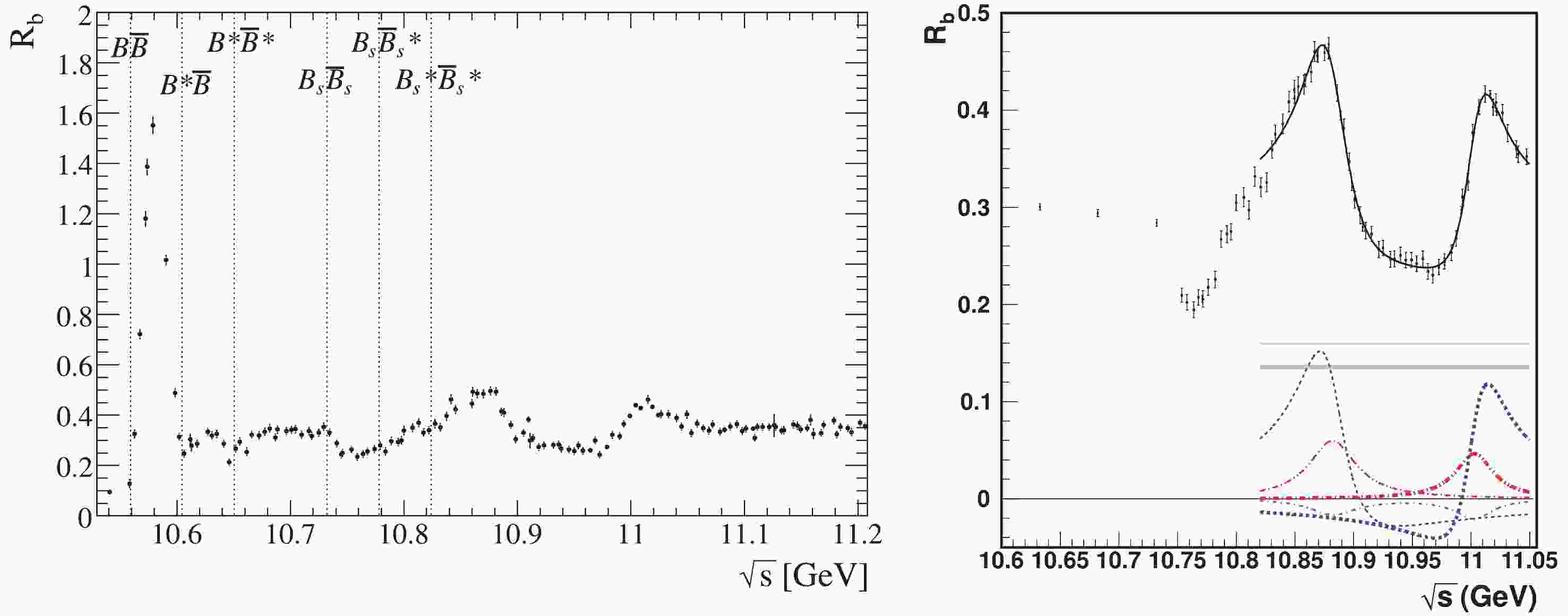
$ {\rm fb}^{-1} $ at the peak$ \sqrt{s} = 10.869 $ GeV, approximately 1$ {\rm fb}^{-1} $ at each of the 16 energy points between 10.63 and 11.02 GeV, and 50$ {\rm pb}^{-1} $ at each of the 61 points taken in 5 MeV steps between 10.75 and 11.05 GeV. The non-resonant$ q\bar q $ continuum$ (q\in\{u,d,s,c\}) $ background is obtained using a 1.03$ {\rm fb}^{-1} $ data sample taken at$ \sqrt{s} = 10.52 $ GeV. The Belle experiment supplied a data file of$ R_b $ with the ISR-produced$ \Upsilon(1S) $ ,$ \Upsilon(2S) $ , and$ \Upsilon(3S) $ states removed (defined as$ R_b^\prime $ in the Belle paper [6]).The BaBar and Belle measurements [5, 6] are shown in Fig. 1. Notice that the definitions of
$ R_b $ are different in these papers. After removing the ISR contribution of the narrow$ \Upsilon $ states from BaBar results, the$ R_b $ values and the comparison between the two experiments are shown in Fig. 2. In the following analysis,$ R_b $ refers to the results after removing the ISR contribution of the narrow$ \Upsilon $ states,$ R_b^{\rm {dre}} $ refers to the dressed cross section after the ISR correction is applied, and$ R_b^{{\rm{B}}} $ refers to the Born cross section after the ISR and VP corrections are applied.
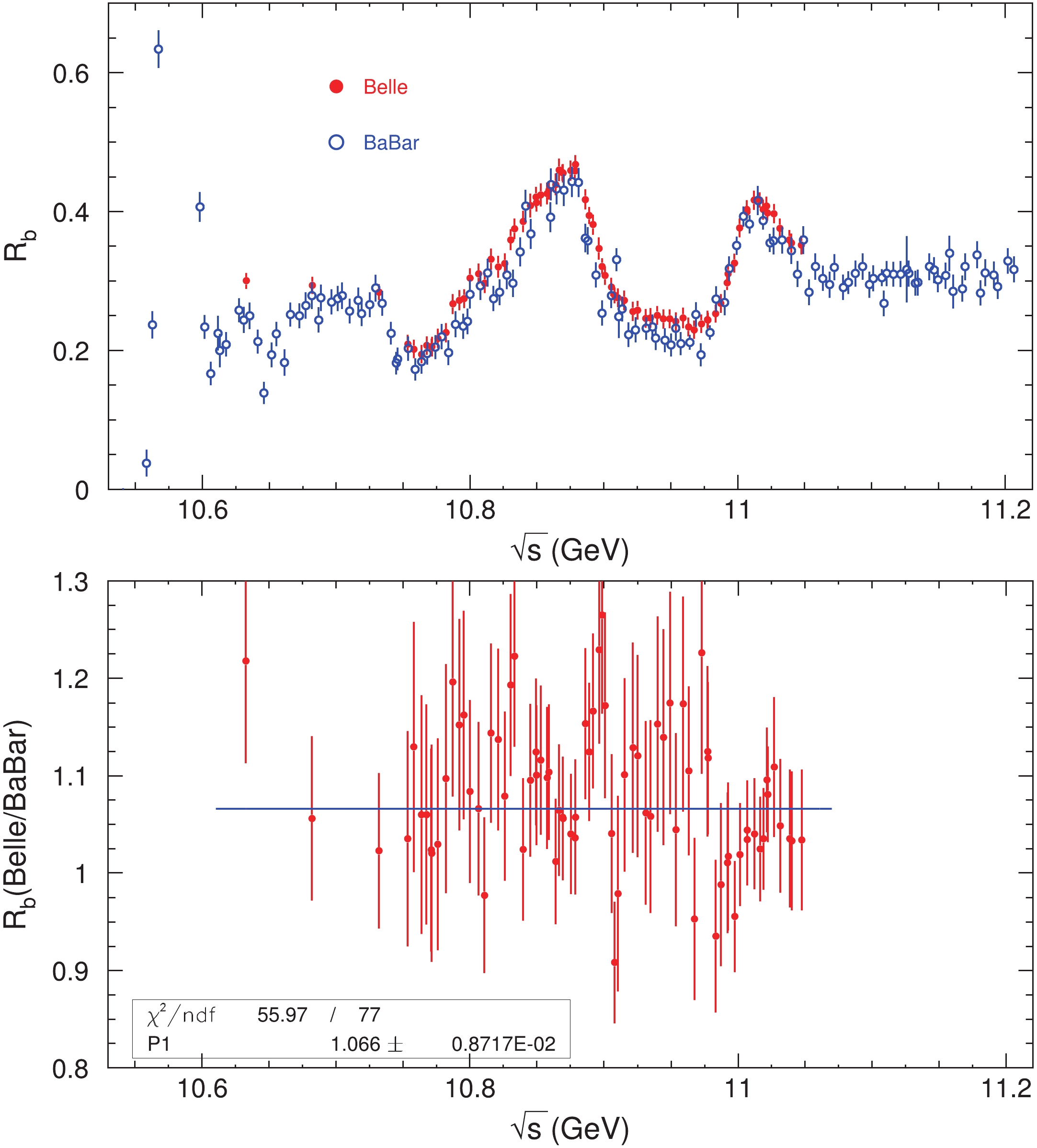
Figure 2. (color online) Comparison of
$ R_b $ data from the BaBar (open cycles) and Belle (red dots) [top panel] experiments and the ratio of$ R_b $ between the Belle and BaBar measurements [bottom panel]. Error bars are combined statistical and systematic errors, and the line is a fit to the ratio of the Belle and BaBar measurements.We can see from Fig. 2 that the Belle results are systematically larger than the BaBar measurements. To obtain the size of the systematic difference, we calculate the ratio between the Belle and BaBar measurements in the energy region covered by both experiments. Figure 2 shows the ratio of
$ R_b $ between the Belle and BaBar measurements; the ratios are fitted with a constant with a good fit quality,$\chi^2/{ndf} = 56/77$ , where${ndf}$ is the number of degrees of freedom. This indicates that the Belle and BaBar measurements differ by a factor of$ f = 1.066\pm 0.009, $

(21) which is more than
$ 7\sigma $ from 1 if they are the same. -
The BaBar experiment measured the
$ R_b $ above 11.1 GeV, which is very flat. This indicates that the bottomonium resonance region has been passed and the flat continuum region has been reached. At the CM energy well above the open-bottom threshold, the R values (the total cross section of$ e^+e^- $ annihilation) and$ R_b $ can be calculated with pQCD with five different flavors of quarks, and this can be compared with the BaBar measurement. If we assume that the difference in$ R_b $ between Belle and BaBar can be extrapolated to the energy region above 11.1 GeV, by comparing the expected Belle measurements in this energy region and the pQCD expectation, we can check the normalization of the Belle data.To compare
$ R_b $ with pQCD calculation, the ISR correction and VP correction should be applied to the Belle and BaBar measurements, since pQCD calculates the Born cross sections. Using the ISR correction factors (point-by-point correction, average correction factor$ 1+\delta\approx 0.901 $ above 11.1 GeV) and VP factors ($ \frac{1}{|1-\Pi|^2}\approx 1.076 $ ) calculated below, a fit to$ R_b^{{\rm{B}}} $ from the BaBar experiment for CM energies between 11.10 and 11.21 GeV yields$ R_b^{{\rm{B}}} = 0.316\pm 0.011 $ , with the error dominated by the common systematic error.Assuming Eq. (21) applies to
$ R_b^{{\rm{B}}} $ at CM energy above 11.1 GeV for the Belle measurement, we extrapolate the Belle measurement to this energy region so that we would expect$ \begin{split} R_b^{{\rm{B}}} =& (0.316\pm 0.011)\times (1.066\pm 0.009) \\=& 0.337\pm 0.012. \end{split}$

(22) Calculating
$ R_b^{{\rm{B}}} $ and the total continuum R values from$ udsc $ -quarks in pQCD according to Eq. (18), we find that$ R_b^{{\rm{B}}} $ is almost constant for CM energy between 11.10 GeV and 11.21 GeV, at 0.351 with negligible uncertainty compared with the experimental measurement; and$ R^B_{udsc} $ can be well parametrized as a linear function of CM energy ($ \sqrt{s} $ in GeV) between 10 and 12 GeV, i.e.,$ R^B_{udsc} = 3.5769-4.1249\times 10^{-3}\sqrt{s}. $

(23) Figure 3 shows the comparison between the BaBar measurements, Belle expected, and pQCD calculated
$ R_b^{{\rm{B}}} $ ; we can find that the Belle data agree with the pQCD calculation reasonably well (within approximately$ 1\sigma $ ; the common error of the Belle measurements at high energy is approximately$ \pm 0.011 $ , similar to the BaBar measurements), while the BaBar measurements are about$ 3\sigma $ lower than the pQCD calculation. As a consequence, we assume the BaBar measurement suffers from a normalization bias, and the Belle measurement is normalized properly. In the analysis below, we increase the BaBar measurements by the factor f in Eq. (21) and combine them with the Belle measurements to treat them as a single data set. The normalized and combined data are shown in Fig. 4.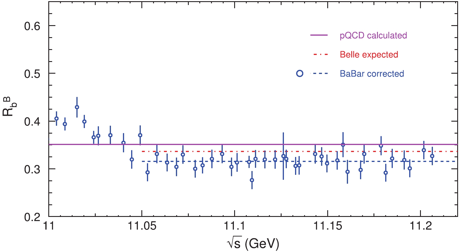
Figure 3. (color online) The
$ R_b^{{\rm{B}}} $ data from BaBar after ISR and VP corrections (open cycles) and the fit with a constant function (blue dashed line,$ R_b^{{\rm{B}}} = 0.316 $ ), expected Belle results (red dash-dotted line,$R_b^{{\rm{B}}} = 0.316\times $ $1.066 = 0.337$ ), and pQCD calculation (pink line,$ R_b^{{\rm{B}}} = 0.351 $ ). Error bars are combined statistical and systematic errors.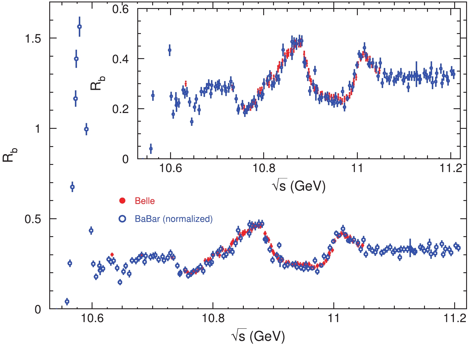
Figure 4. (color online) Normalized
$ R_b $ data from BaBar (open cycles) and Belle (red dots), which will be treated as a single data set. Error bars are combined statistical and systematic errors.In the remainder of this work, the threshold of open-bottom production is set to be 10.5585 GeV, larger than the first two energy points in the BaBar experiment. Therefore, these two data were omitted in our analysis.
-
To calculate the ISR correction factors, the measured
$ R_b $ will be used as the input. To avoid the point-to-point statistical fluctuation, one may parametrize the line shape with a smooth curve. There is no known function describing the line shape a priori, so one may parametrize the line shape with any possible combination of smooth curves.We use the “robust locally weighted regression” or “LOWESS” method to smooth the experimental measurements. The principal routine of LOWESS computes the smoothed values using the method described in Ref. [22]. This method works very well only for slowly varying data, which makes the procedure at the
$ \Upsilon(4S) $ region work improperly. As a consequence, we use the data points directly for$ \sqrt{s}<10.66 $ GeV and use the smoothed data for the other data points. Figure 5 shows the smoothed$ R_b $ , which looks very reasonable.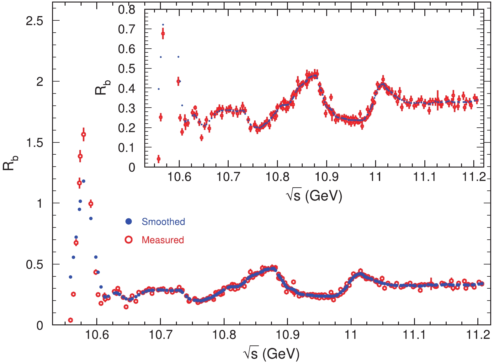
Figure 5. (color online) Belle and BaBar combined
$ R_b $ data (red circles with error bars) and the results after smoothing (blue dots). Error bars are combined statistical and systematic errors.In the following analysis, we use a straight line to connect two neighboring points. As these points are after smoothing and the step is not big, there is no big jump between neighboring points, so we do not expect significant difference between a straight line and a smooth curve.
-
We follow the procedure defined in Eqs. (7), (8), and (9) to calculate the ISR correction factors. In doing this for the experimental data, we assume the detection efficiencies for
$ b\bar{b} $ events without ISR and those with different energies of ISR photons have been estimated reliably within the quoted systematic uncertainties in both the BaBar [5] and Belle experiments [6]. The iteration is continued until the difference between two consecutive results is less than 1% of the statistical error of the observed$ R_b $ .In the energy region where the cross section varies smoothly, the ISR correction factors become stable after a few iterations, whereas in the
$ \Upsilon(4S) $ energy region, due to the rapid change of the cross section in the narrow energy region, the ISR correction factors only converge to within 1% after more than ten iterations. We iterate 20 times, and the maximum difference is less than 0.5% within the full energy region. Figure 6 shows the final ISR factors as well as the corrected$ R_b^{\rm {dre}} $ values.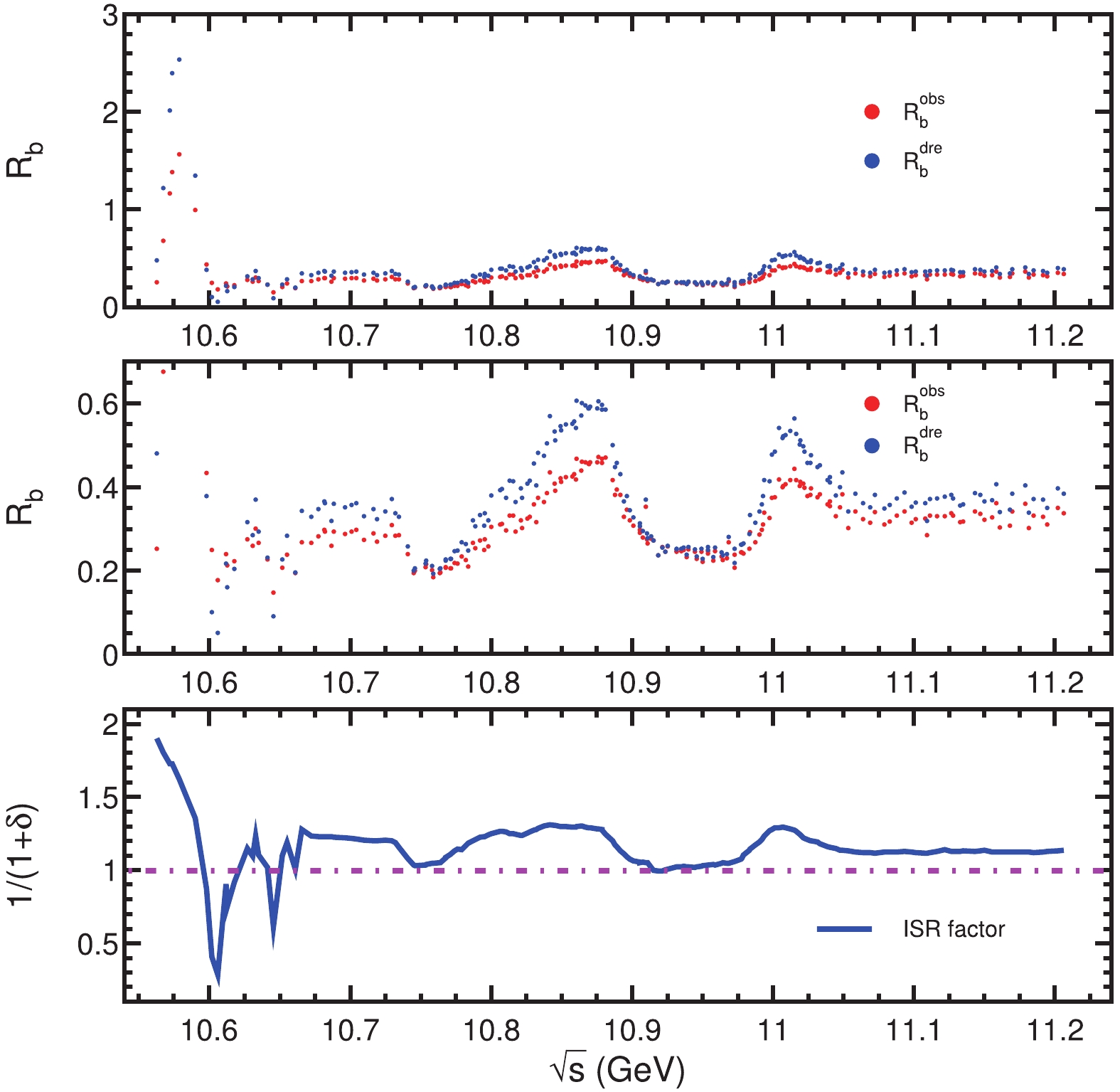
Figure 6. (color online) Normalized
$ R_b $ (red in the top two panels) and ISR-corrected$ R_b $ (or$ R_b^{\rm {dre}} $ , blue in the top two panels); errors are not shown. The bottom panel shows the ISR correction factor. -
Taking
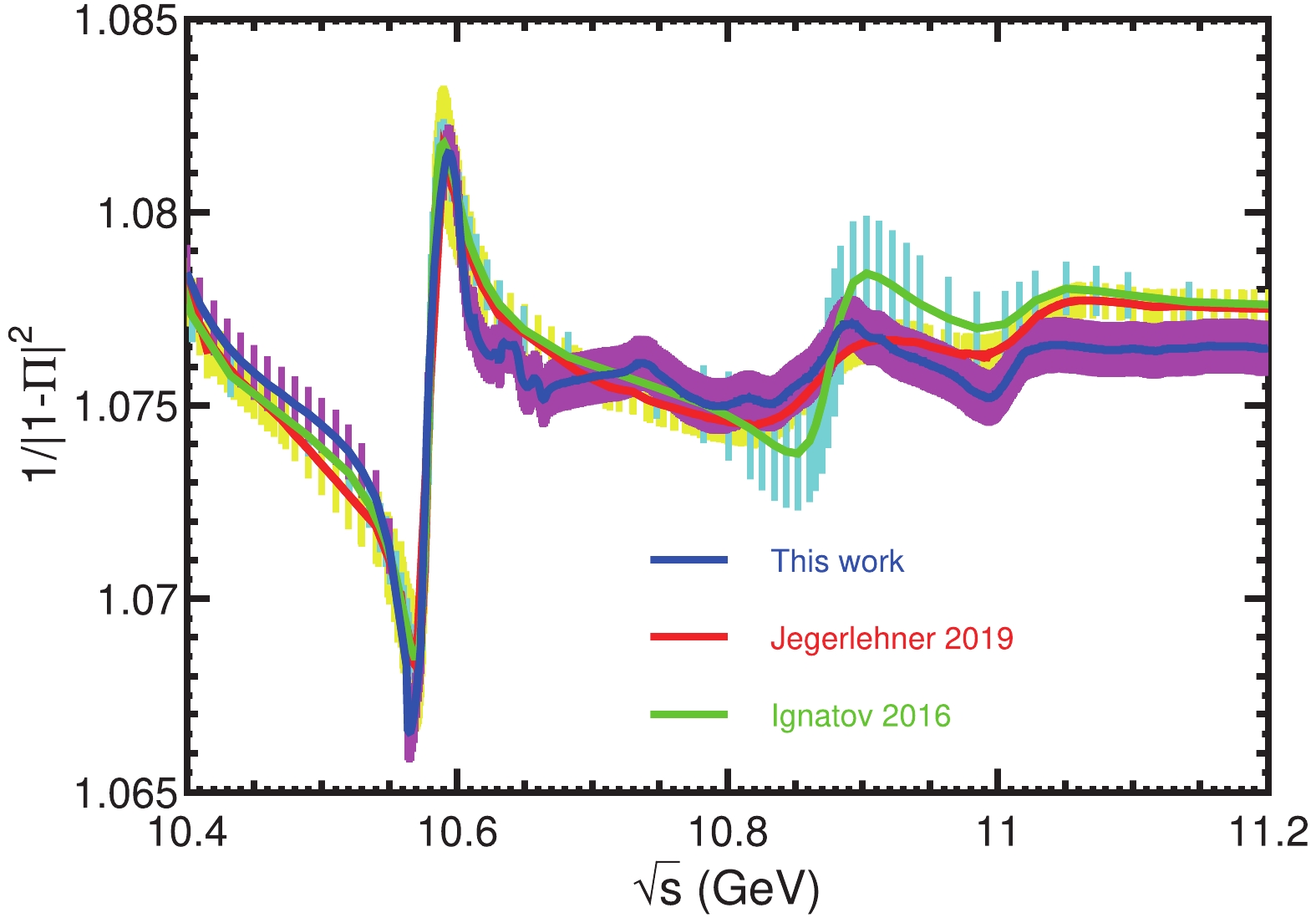
$ R_b^{\rm {dre}} $ , the ISR-corrected$ R_b $ obtained in Sec. 4.1, as the approximation of$ R_b^{{\rm{B}}} $ and adding the pQCD calculation of the$ udsc $ -quark contribution to the R values (refer to Eq. (23)), we calculate the VP factors in the bottomonium energy region. After obtaining the VP factor$ {1}/{|1-\Pi|^2} $ , we use$ R_b^{\rm {dre}}/{1}/{ |1-\Pi|^2} $ as the input to calculate$ {1}/{|1-\Pi|^2} $ again and we iterate this process. After three iterations, the VP factor$ {1}/{|1-\Pi|^2} $ becomes stable so we take the values from this round as the final results, and we obtain$ R_b^{{\rm{B}}} $ with Eq. (20). Figure 7 shows the VP factors from this calculation.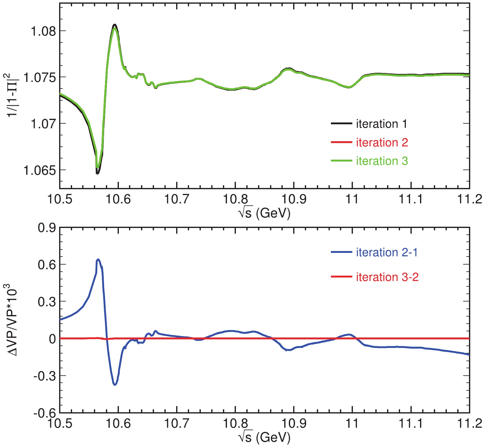
Figure 7. (color online) VP factors from three iterations (top) and the difference between two iterations (bottom). Notice that the difference between the second and third iterations is very small and the curves for the VP factors are almost indistinguishable.
-
In the previous two subsections we obtained the ISR correction factor and VP factor and in turn the Born
$ R_b^{{\rm{B}}} $ via Eq. (20). During the calculation, however, only the central values of the observed$ R_b $ are used. Instead of just scaling the errors of the original measurements by the obtained ISR correction factors and the VP factors, we perform a toy Monte Carlo sampling to investigate how the errors (both statistical and systematic) of the original measurements impact the obtained$ R_b^{{\rm{B}}} $ .At each energy point where the Belle or BaBar measurement [5, 6] was performed, we perform 10,000 samplings of the observed
$ R_b $ according to a Gaussian distribution for which the mean value and standard deviation are the central value and statistical error of the observed$ R_b $ , respectively. These samples will be used to estimate the statistical errors of the deduced quantities. In addition, the uncommon systematic errors are added to the samples in the same way. For the common systematic error, the same error is added to each sample at all energy points in the Belle or BaBar experiment. These samples, with both statistical and systematic errors considered, will yield the total errors of the deduced quantities. In the energy regions$ 0.36<\sqrt{s}<2.0 $ GeV and$ 3.7<\sqrt{s}<5.0 $ GeV, the data from the PDG compilation [1, 16] and BES collaboration [17, 18] are assumed to be completely correlated when we perform the sampling.With each sample as input, we repeat the calculation described in the previous two subsections to obtain the ISR correction factor, VP factor, and
$ R_b^{{\rm{B}}} $ for this sample. Finally, a distribution of$ R_b^{{\rm{B}}} $ at each energy point is observed, as are the ISR correction factor and VP factor. We find that these distributions also satisfy a Gaussian distribution well, so the fitted mean and standard deviation are taken as the central value and error of the corresponding quantities, respectively. The covariances of the distributions of Born and dressed cross sections at different energy points are also available in the supplementary material [23]. These covariances are useful in calculations where$ R_b^{\rm B} $ or$ R_b^{\rm {dre}} $ are inputs, such as extracting the resonant parameters of$ Y(10750) $ ,$ \Upsilon(5S) $ , and$ \Upsilon(6S) $ by fitting$ R_b^{\rm {dre}} $ .Recall that we smoothed the observed R values using the “LOWESS” method before we calculated the dressed and Born ones. In principle, one can use different methods to smooth the data, which will result in uncertainty of the final results. We test another smoothing method, “Smoothing spline” [24], and find that such uncertainty is negligible when compared with the original errors.
-
After all the above operations, we obtain
$ R_b^{{\rm{B}}} $ as well as its total uncertainty from the combined BaBar and Belle measurements as shown in Fig. 8 and Table A1 in the Appendix A. We find that the$ R_b^{{\rm{B}}} $ values are very different from the$ R_b $ values reported from the original publications [5, 6], and the differences are energy dependent. Common features are that the peaks are even higher and the valleys become deeper, the two dips at the$ B\bar{B^*}+c.c. $ and$ B^*\bar{B^*} $ thresholds are more significant, the peaks corresponding to the$ \Upsilon(5S) $ and$ \Upsilon(6S) $ increase significantly, and there is a prominent dip at 10.75 GeV.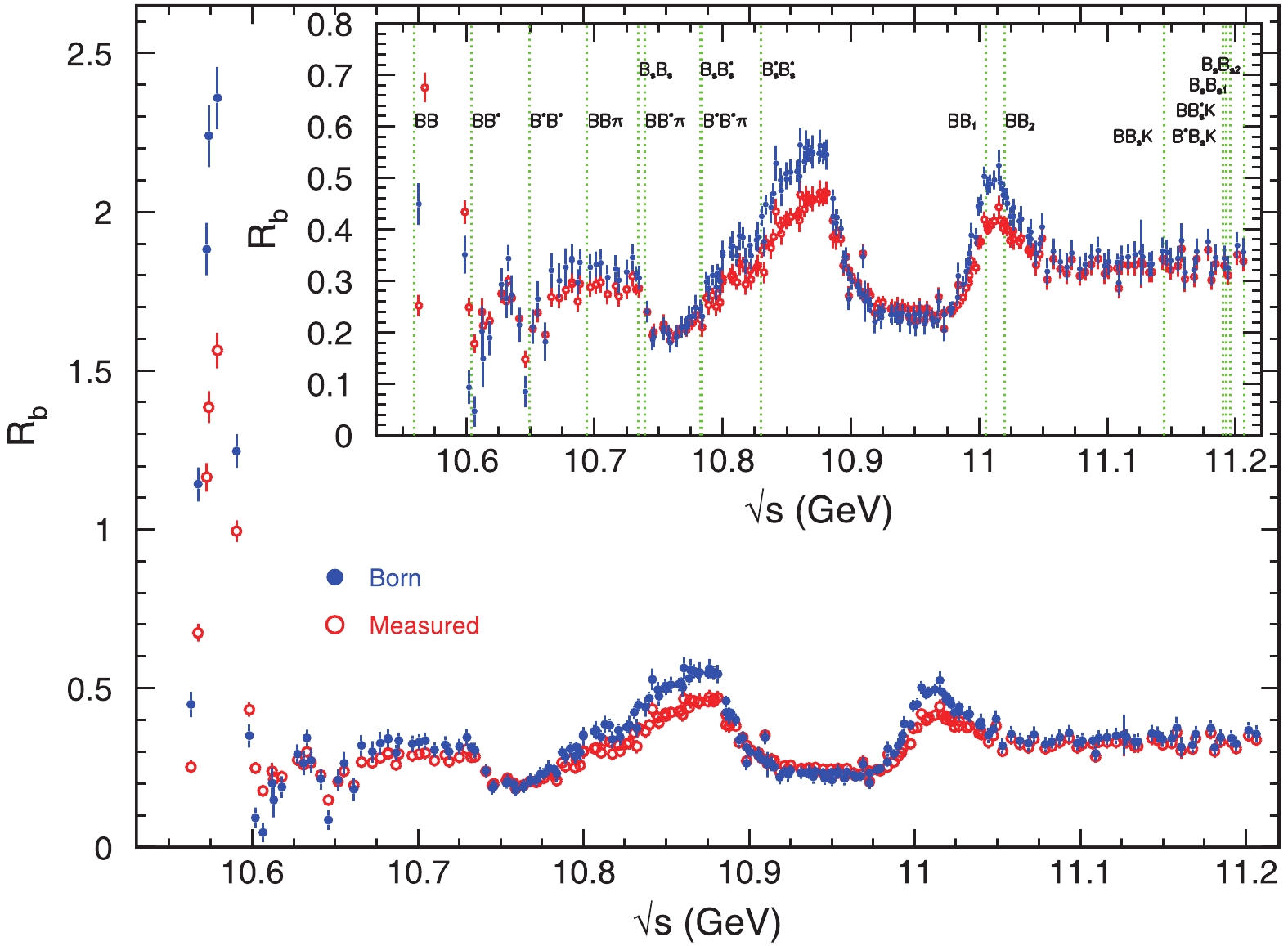
Figure 8. (color online) Comparison of measured
$ R_b $ (open cycles) and Born$ R_b^{{\rm{B}}} $ (solid dots). The error bars are the combined statistical and systematic errors. The dotted vertical lines are the thresholds for bottom meson productions.The total R value corresponding to the production of
$ udscb $ quarks can be obtained directly by adding the$ R_b^{{\rm{B}}} $ to the$ udsc $ -quark contribution calculated from pQCD, as indicated in Eq. (23). -
From the BaBar and Belle measurements of the observed
$ e^+e^-\to b\bar{b} $ cross sections, we perform ISR correction to obtain the dressed$ e^+e^-\to b\bar{b} $ cross sections from 10.56 to 11.21 GeV. These dressed cross sections are the right ones to be used to determine the resonant parameters of the vector bottomonium states. Together with the R values measured at other energy points and the R values calculated with pQCD, we calculate the VP factors. By applying the VP correction, we obtain the Born cross section of$ e^+e^-\to b\bar{b} $ from the threshold to 11.21 GeV. These cross sections can be used for all calculations related to the photon propagator, such as$ a_\mu $ , the$ \mu $ anomalous magnetic moment, and$ \alpha(s) $ , the running coupling constant of QED [2, 3].In the following parts of this section, we discuss the usage of the data obtained in this study.
-
The VP factors have been calculated by many groups [14, 25-28], using both experimental data and various theoretical inputs when the data are not available or less precise. Different techniques of handling the discrete data points and correcting possible biases in the data have been developed. All these different treatments yield very similar results on hadronic contribution to
$ a_\mu $ and on the running of$ \alpha $ at$ M_{Z^0}^2 $ , which indicates that the methods are all essentially applicable with the current precision of data.Previous calculations of the VP factors in the bottomonium energy region used either the resonant parameters of
$ \Upsilon(4S) $ ,$ \Upsilon(5S) $ , and$ \Upsilon(6S) $ reported by previous experiments [7, 8], which are very crude [26, 27], or the experimental data from previous experiments [7, 8], which gave the observed cross sections [28]. We recalculate the VP factors using the$ R_b^{{\rm{B}}} $ obtained in this analysis, based on high-precision data from the BaBar and Belle experiments [5, 6], with the ISR correction and VP factors properly considered. Although these new data have little effect on the VP factors far from the bottomonium energy region, they do change the VP factors in the bottomonium energy region as shown in Fig. 9. The difference between this and previous calculations [26, 27] is visible at some energies, although all the calculations agree within the errors. -
There are very clear structures in the
$ R_b^{{\rm{B}}} $ distribution shown in Fig. 8. From low to high energy, we identify$ \Upsilon(4S) $ at 10.58 GeV, dips due to the$ B\bar{B^*}+c.c. $ and$ B^*\bar{B^*} $ thresholds at 10.61 and 10.65 GeV, respectively, a dip at 10.75 GeV that may correspond to$ Y(10750) $ [29], and$ \Upsilon(5S) $ and$ \Upsilon(6S) $ at 10.89 and 11.02 GeV, respectively.The observed
$ R_b $ values were used to extract the resonant parameters of the$ \Upsilon(5S) $ and$ \Upsilon(6S) $ in the BaBar [5] and Belle [6] publications. As the ISR correction effect is significant and energy dependent, this suggests that the fit results are not reliable. To avoid the dip at approximately 10.75 GeV, both BaBar and Belle fitted data above 10.80 GeV only. A recent study of$ e^+e^-\to \pi^+\pi^-\Upsilon $ revealed a new state,$ Y(10750) $ , with a mass of$ (10752.7\pm 5.9^{+0.7}_{-1.1}) $ MeV/$ c^2 $ and width$ (35.5^{+17.6}_{-11.3}{}^{+3.9}_{-3.3}) $ MeV [29], at exactly the position of the dip in$ R_b^{{\rm{B}}} $ . This indicates that the dip is very likely to be produced by the interference between a Breit–Wigner function and a smooth background component.We perform a least-square fit to the dressed
$ e^+e^-\to b\bar{b} $ cross sections ($ \sigma^{\rm {dre}} = \dfrac{\sigma^B}{|1-\Pi|^2} $ ) above 10.68 GeV with the coherent sum of a continuum amplitude (proportional to$ 1/\sqrt{s} $ ) and three Breit–Wigner functions with constant widths representing the structures at 10.75, 10.89, and 11.02 GeV. The Breit–Wigner function is$ {\rm {BW}} = {\rm e}^{{\rm i}\phi}\frac{\sqrt{12\pi\Gamma_{ e^+e^-}\Gamma}}{s-m^2+{\rm i}m\Gamma}, $

where m,
$ \Gamma $ ,$ \Gamma_{ e^+e^-} $ , and$ \phi $ are the mass, total width, and electronic partial width of the resonance, and the relative phase between the resonance and the real continuum amplitude, respectively, and they are all free parameters in the fits.Eight sets of solutions are found from the fit [30], with identical total fit curves, identical fit quality (
$ \chi^2 = 274 $ with 188 data points and 13 free parameters), and identical masses and widths for the same resonance, but with significantly different$ \Gamma_{ e^+e^-} $ and$ \phi $ .Figure 10 shows one of the solutions of the fit, and Table 1 lists the resonant parameters from the eight solutions of the fit. The masses and widths of the resonances agree with those from Ref. [29] but with improved precision because of the superior measurements used in this work compared with those in exclusive
$ e^+e^-\to \pi^+\pi^-\Upsilon $ analyses. The$ \Gamma_{ e^+e^-} $ values determined from this study allow us to extract the branching fractions of$ \pi^+\pi^-\Upsilon $ of these resonances by combining the information reported in Ref. [29], and to understand the nature of these vector states [31-35].Solution Parameter $ Y(10750) $ 

$ \Upsilon(5S) $ 

$ \Upsilon(6S) $ 

1–8 Mass/(MeV/ $\rm c^2 $ )

$ 10761\pm 2 $ 

$ 10882\pm 1 $ 

$ 11001\pm 1 $ 

Width/MeV $ 48.5\pm 3.0 $ 

$ 49.5\pm 1.5 $ 

$ 35.1\pm 1.2 $ 

1 $ \Gamma_{ e^+e^-} $ /eV

$ 10.7\pm 0.9 $ 

$ 21.3\pm 1.0 $ 

$ 9.8\pm 0.5 $ 

$ \phi $ /(°)

$ 260\pm 3 $ 

$ 144\pm 2 $ 

$ 34\pm 3 $ 

2 $ \Gamma_{ e^+e^-} $ /eV

$ 11.1\pm 0.9 $ 

$ 24.8\pm 1.3 $ 

$ 307\pm 9 $ 

$ \phi $ /(°)

$ 270\pm 3 $ 

$ 164\pm 2 $ 

$ 280\pm 1 $ 

3 $ \Gamma_{ e^+e^-} $ /eV

$ 12.6\pm 1.1 $ 

$ 479\pm 14 $ 

$ 11.5\pm 0.6 $ 

$ \phi $ /(°)

$ 295\pm 3 $ 

$ 254\pm 1 $ 

$ 3\pm 3 $ 

4 $ \Gamma_{ e^+e^-} $ /eV

$ 13.0\pm 1.1 $ 

$ 558\pm 19 $ 

$ 363\pm 13 $ 

$ \phi $ /(°)

$ 296\pm 3 $ 

$ 274\pm 1 $ 

$ 249\pm 1 $ 

5 $ \Gamma_{ e^+e^-} $ /eV

$ 324\pm 24 $ 

$ 23.7\pm 1.2 $ 

$ 10.0\pm 0.5 $ 

$ \phi $ /(°)

$ 265\pm 1 $ 

$ 129\pm 2 $ 

$ 26\pm 3 $ 

6 $ \Gamma_{ e^+e^-} $ /eV

$ 336\pm 27 $ 

$ 27.6\pm 1.6 $ 

$ 314\pm 10 $ 

$ \phi $ /(°)

$ 275\pm 1 $ 

$ 149\pm 2 $ 

$ 272\pm 1 $ 

7 $ \Gamma_{ e^+e^-} $ /eV

$ 380\pm 32 $ 

$ 534\pm 18 $ 

$ 11.8\pm 0.6 $ 

$ \phi $ /(°)

$ 291\pm 1 $ 

$ 239\pm 1 $ 

$ 355\pm 3 $ 

8 $ \Gamma_{ e^+e^-} $ /eV

$ 394\pm 34 $ 

$ 622\pm 25 $ 

$ 370\pm 14 $ 

$ \phi $ /(°)

$ 301\pm 1 $ 

$ 259\pm 2 $ 

$ 241\pm 1 $ 

Table 1. Resonant parameters from the fit to dressed cross sections. There are eight solutions with identical fit quality, and the masses and widths of the resonances are identical in all the solutions. The uncertainties are combined statistical and systematic uncertainties in experimental measurements.
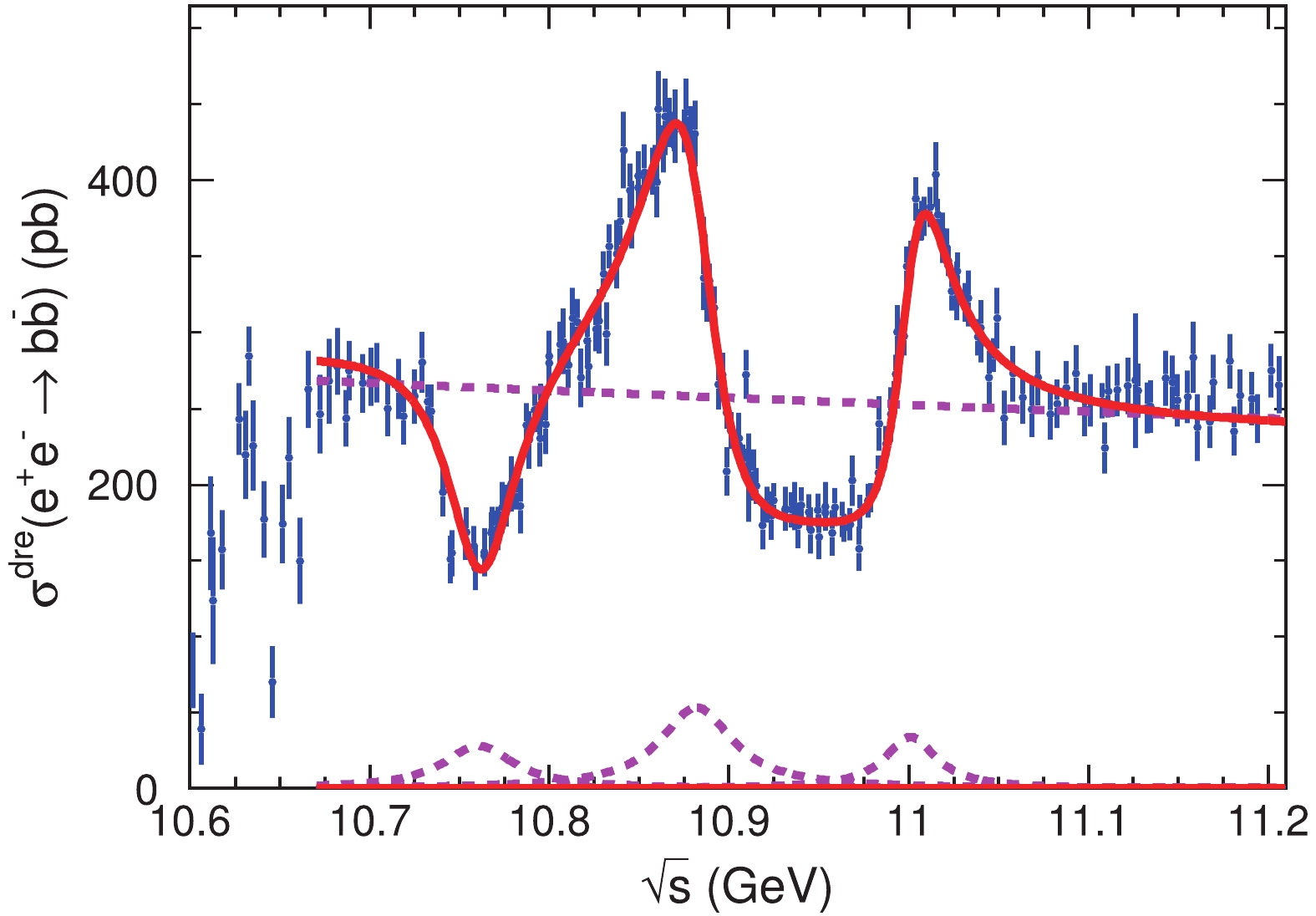
Figure 10. (color online) Fit to the dressed cross sections with coherent sum of a continuum amplitude and three Breit–Wigner functions. The solid curve is the total fit, and the dashed ones correspond to each of the four components from Sol. 1 in Table 1. The magnitudes of these components are different in different solutions.
In this analysis, we assumed that all the resonances are Breit–Wigner functions with constant widths and the continuum term is a smooth curve in the full energy region, and they interfere with each other completely. In fact, the
$ R_b^{{\rm{B}}} $ or total cross section has contributions from different modes, including open-bottom and hidden-bottom final states. The parametrization of the line shape should be very complicated due to the coupled-channel effect [36] and the presence of many open-bottom thresholds:$ B\bar{B} $ ,$ B\bar{B^*}+c.c. $ ,$ B^*\bar{B^*} $ ,$ B_s\bar{B_s} $ ,$ B_s\bar{B_s^*}+c.c. $ ,$ B_s^*\bar{B_s^*} $ ,$ B\bar{B_1}+c.c. $ ,$ B^*\bar{B_0}+c.c. $ ,$ B^*\bar{B_1}+c.c. $ ,$ B\bar{B_2}+c.c. $ , etc., and even$ \pi Z_b(10610) $ and$ \pi Z_b(10650) $ . The situation becomes somewhat simpler in a single final state like$ \pi^+\pi^-\Upsilon(nS) $ ($ n = 1,\, 2,\, 3 $ ) [6] and$ \pi^+\pi^- h_b(mP) $ ($ m = 1,\, 2 $ ) [37] although the intermediate structure in the three-body final state is also complicated. The results from these fits may change dramatically by including more information on each exclusive mode.We also attempt to add one more Breit–Wigner function to fit the cross sections; the fit quality improves slightly with a state at
$ m = (10848\pm 9) $ MeV/$\rm c^2$ with a width of$ (28\pm 14) $ MeV, a state at$ m = (10831\pm 1) $ MeV/$\rm c^2$ with a width of$ (14\pm 5) $ MeV, or a state at$ m = (11065\pm 23) $ MeV/$\rm c^2$ with a width of$ (73\pm 37) $ MeV. In all these cases, the significance of the additional state is less than$ 4\sigma $ .The data obtained in this analysis can be used to extract resonant parameters of these states if a better parametrization of the cross sections is developed.
-
The experimentally observed
$ e^+e^-\to \mu^+\mu^- $ cross section, with radiative correction, is expressed as$ \sigma(s)( e^+e^-\to \mu^+\mu^-) = \int^{x_m}_0 \frac{4\pi\alpha^2}{3s(1-x)} \frac{F(x,s)}{|1-\Pi(s(1-x))|^2} {\rm d}x, $

(24) where
$ F(x,s) $ is expressed in Eq. (3), and$ x_m = 1-s_m/s $ , with$ \sqrt{s_m} $ the required minimum invariant mass of the$ \mu $ pair in the event selection. Here, the mass of$ \mu $ is neglected for charm and beauty factories. In Eq. (24), the cross section is calculated by QED without any ambiguity except the vacuum polarization$ \Pi(s) $ which is expressed by Eqs. (10)-(15), with the hadronic contribution depending on the experimental measured data as input.If the
$ e^+e^-\to \mu^+\mu^- $ cross section is measured to a high precision, then$ \Pi(s) $ can be obtained. Thus,$ \Pi(s) $ is measured from the experiment directly [38]. It can then be compared with that calculated by Eqs. (10)-(15). This provides a test of QED at high-luminosity flavor factories. In Eq. (10), the leptonic term$ \Pi_l(s,m^2) $ is expressed in terms of the QED fine structure constant$ \alpha(0) $ and lepton masses, which are all known to very high accuracy, while the hadronic term$ \Pi_h(s) $ must be evaluated with Eq. (15) with the input of experimental measured hadronic cross sections. It is seen in Eq. (15) that$ \Pi_h(s) $ is most sensitive to the hadronic cross section at energies close to s, which can be measured with the same experiment. Therefore, such a test of QED can be performed with two sets of data,$ e^+e^-\to \mu^+\mu^- $ and$ e^+e^-\to {\rm {hadrons}} $ , collected within the same experiment. Any discrepancy would mean that there are missing hadronic final states, or even a final state that escaped detection or is invisible by current detection technology. This provides a test of QED and search for new physics. We propose for it to be included in physics goals in future high-luminosity frontier physics.$\sqrt{s}$ /GeV

$R_b^{\rm B}$ 

$R_b^{\rm{dre}}$ 

$1/(1+\delta)$ 

$1/|1-\Pi|^2$ 

10.5628 0.4498 ± 0.0341 ± 0.0155 0.4799 ± 0.0364 ± 0.0164 1.9009 ± 0.0000 1.0670 ± 0.0008 10.5673 1.1436 ± 0.0399 ± 0.0308 1.2199 ± 0.0425 ± 0.0325 1.8044 ± 0.0074 1.0668 ± 0.0008 10.5723 1.8835 ± 0.0598 ± 0.0487 2.0122 ± 0.0642 ± 0.0516 1.7273 ± 0.0063 1.0683 ± 0.0008 10.5738 2.2419 ± 0.0714 ± 0.0574 2.3981 ± 0.0760 ± 0.0610 1.7294 ± 0.0126 1.0697 ± 0.0008 10.5788 2.3593 ± 0.0700 ± 0.0598 2.5363 ± 0.0750 ± 0.0642 1.6218 ± 0.0082 1.0750 ± 0.0008 10.5903 1.2485 ± 0.0372 ± 0.0323 1.3496 ± 0.0402 ± 0.0350 1.3543 ± 0.0121 1.0809 ± 0.0008 10.5983 0.3508 ± 0.0326 ± 0.0119 0.3791 ± 0.0353 ± 0.0128 0.8728 ± 0.0438 1.0809 ± 0.0008 10.6018 0.0943 ± 0.0289 ± 0.0059 0.1019 ± 0.0312 ± 0.0063 0.4002 ± 0.1016 1.0797 ± 0.0008 10.6063 0.0465 ± 0.0270 ± 0.0053 0.0501 ± 0.0291 ± 0.0057 0.2732 ± 0.1383 1.0779 ± 0.0008 10.6118 0.2022 ± 0.0444 ± 0.0079 0.2178 ± 0.0478 ± 0.0085 0.8942 ± 0.1092 1.0771 ± 0.0008 10.6128 0.1488 ± 0.0498 ± 0.0083 0.1603 ± 0.0536 ± 0.0090 0.7332 ± 0.1801 1.0771 ± 0.0008 10.6178 0.1892 ± 0.0301 ± 0.0082 0.2037 ± 0.0324 ± 0.0089 0.9110 ± 0.0810 1.0765 ± 0.0008 10.6273 0.2938 ± 0.0263 ± 0.0102 0.3162 ± 0.0283 ± 0.0110 1.1466 ± 0.0401 1.0763 ± 0.0008 10.6308 0.2648 ± 0.0331 ± 0.0102 0.2850 ± 0.0356 ± 0.0110 1.0919 ± 0.0638 1.0762 ± 0.0008 10.6328 0.3440 ± 0.0067 ± 0.0228 0.3702 ± 0.0072 ± 0.0245 1.2330 ± 0.0444 1.0763 ± 0.0008 10.6353 0.2728 ± 0.0335 ± 0.0123 0.2937 ± 0.0360 ± 0.0133 1.0989 ± 0.0658 1.0766 ± 0.0008 10.6413 0.2145 ± 0.0293 ± 0.0082 0.2310 ± 0.0315 ± 0.0088 1.0136 ± 0.0666 1.0765 ± 0.0008 10.6458 0.0848 ± 0.0287 ± 0.0048 0.0912 ± 0.0308 ± 0.0051 0.6015 ± 0.1485 1.0761 ± 0.0008 10.6518 0.2120 ± 0.0297 ± 0.0103 0.2279 ± 0.0319 ± 0.0111 1.0931 ± 0.0681 1.0754 ± 0.0008 10.6553 0.2637 ± 0.0312 ± 0.0103 0.2836 ± 0.0335 ± 0.0111 1.1868 ± 0.0602 1.0755 ± 0.0008 10.6613 0.1820 ± 0.0335 ± 0.0086 0.1957 ± 0.0360 ± 0.0093 0.9961 ± 0.0892 1.0755 ± 0.0008 10.6659 0.3194 ± 0.0255 ± 0.0116 0.3434 ± 0.0275 ± 0.0125 1.2768 ± 0.0358 1.0754 ± 0.0008 10.6724 0.3059 ± 0.0207 ± 0.0105 0.3290 ± 0.0223 ± 0.0113 1.2326 ± 0.0118 1.0754 ± 0.0008 10.6774 0.3236 ± 0.0218 ± 0.0102 0.3480 ± 0.0235 ± 0.0110 1.2307 ± 0.0104 1.0755 ± 0.0008 10.6819 0.3405 ± 0.0225 ± 0.0101 0.3662 ± 0.0241 ± 0.0109 1.2306 ± 0.0128 1.0755 ± 0.0008 10.6820 0.3364 ± 0.0040 ± 0.0148 0.3618 ± 0.0043 ± 0.0159 1.2306 ± 0.0128 1.0755 ± 0.0008 10.6869 0.2975 ± 0.0209 ± 0.0103 0.3200 ± 0.0225 ± 0.0110 1.2273 ± 0.0130 1.0756 ± 0.0008 Continued on next page Table A1. Final results of Born cross section
$R_b^{\rm B}$ and dressed cross section$R_b^{\rm{dre}}$ , together with the ISR correction factors and vacuum polarization factors. The first error of$R_b^{\rm B}$ and$R_b^{\rm{dre}}$ is statistical and the second is systematic. The errors of the ISR factor and VP factor are combined statistical and systematic errors.
Hadronic cross section of
${ {e^+e^-}}$
annihilation at bottomonium energy region
- Received Date: 2020-03-01
- Available Online: 2020-08-01
Abstract: The Born cross section and dressed cross section of


 DownLoad: