


 Abstract
 HTML
HTML Reference
 Related
 PDF
PDF


-
Double beta decay (hereafter
$ \beta\beta $ -decay) is a rare decay that occurs under nuclear circumstance. Its possible mode, called as neutrinoless double beta decay (hereafter$ 0\nu\beta\beta $ ), provides insights into the physics beyond the standard model. Such a decay mode would provide clear evidence of the lepton number violation. However, the discovery itself is not enough to determine the exact mechanism of this violation. Therefore, further investigations on the underlying physics are needed after the discovery of this rare process. Different methods have been proposed for probing the underlying new physics, such as comparisons of the half-lives of various nuclei or of the decays to ground and excited states [1]. Recent surveys show that the decays among different nuclei may be correlated [2] for selected mechanisms, such as light and heavy-mass mechanisms. Meanwhile, the relative decay width to$ 2^+ $ states may be a better way to distinguish between models in the presence of right-handed weak currents [3, 4]. However, to describe such a process, one needs reliable and capable modern nuclear many-body methods. To test the reliability of these methods, we first perform our many-body calculations on double beta decay with neutrinos to the first$ 2^+ $ excited states. These results will also help in the search of such a mode by various collaborations [5, 6].The double beta decay named as two-neutrino double beta decay (2
$ \nu\beta\beta $ ) transforms an even–even nucleus$ {}^{A}X_N $ to a neighboring even–even nucleus$ {}^{A}Y_{N-2} $ with the emission of two electrons and two anti-electron-neutrinos. Owing to angular momentum conservation, the change in the angular momentum of the decaying nucleus is the sum of the angular momenta of the four emitted leptons. For the$ 2\nu\beta\beta $ -decay, the electrons and the neutrinos are dominated by s-partial waves because they have relatively long wavelengths compared to the nuclear radius, owing to their small momenta. Therefore, for the leading order contribution to the decay, the summed angular momentum of the outgoing leptons from the$ \beta\beta $ -decay can have the values of 0, 1, and 2 only. If we search the nuclear chart, we find that there are only a limited number of excited states of the double beta decay daughter nuclei within the$ Q_{\beta\beta} $ -value windows. They have spin-parities$ 2^+ $ and$ 0^+ $ only. Thus, for many$ \beta\beta $ -decay candidates with large enough$ Q_{\beta\beta} $ values, there exist possibilities of decays to the first$ 2^+ $ states ($ 2^+_1 $ ) of the daughter nuclei. All these decays are suppressed by the large energy denominator [3] compared to that of the$ 2\nu\beta\beta $ decay to the ground states. Therefore, they have small branch ratios and low detectability [5]. Thus, precise predictions are helpful to experimentalists. Despite these, measurements of these decays can help to improve nuclear theories and solve problems in nuclear structure calculations, such as the quenching of$ g_A $ . There are already reports in the literature [7-13], using the Shell model and the quasi-particle random phase approximation (QRPA), of investigations of this issue. However, the deviations from model to model are still large; usually, they differ by several orders of magnitude. In this study, by isospin restoration [14, 15], we systematically investigate this issue. By studying the nuclear matrix element (NME) dependence on the particle–particle (pp) interaction strength of both isoscalar and isovector channels using an enlarged model space, we try to understand the uncertainties in the QRPA calculations. We also provide reliable estimations of half-lives with the newly calculated phase space factors (PSFs) from numerical electron wavefunctions [16]. These predicted half-lives are then compared to the current experimental lower limits to explore the discovery potential of different nuclei.This article is organized as follows. In Sec. 2, we provide a brief introduction of the QRPA method and the details of the NMEs and the PSF calculations. In Sec. 3, we present detailed results, followed by conclusions in Sec. 4.
-
The half-life of the
$ \beta\beta $ -decay to the$ 2^+_1 $ states of the daughter nuclei is expressed in a compact form as [3]${[\tau _{1/2}^{2\nu }({0^ + } \to {2^ + })]^{ - 1}} = G_{2\nu }^{{2^ + }}g_A^4|M_{2\nu }^{2 + }{|^2},$

(1) where
$ G_{2\nu}^{2^+} $ is the PSF for the emitted electrons and neutrinos, and$ M^{2^+}_{2\nu} $ is the NME. Unlike normal conventions, we take the axial coupling constant,$ g_A $ , outside the PSF.The PSF can be calculated by integrating over the lepton momenta [3, 17] as follows:
$\begin{split} G_{2\nu }^{{2^ + }} =& \frac{{2{{\tilde A}^6}}}{{\ln 2}}\int_{{m_e}}^{Q_{\beta \beta }^{{2^ + }} + {m_e}} {\int_{{m_e}}^{Q_{\beta \beta }^{{2^ + }} + {m_e} - {\epsilon _1}} {\int_0^{Q_{\beta \beta }^{{2^ + }} - {\epsilon _1} - {\epsilon _2}} {} } } \\ & \times f_{11}^{(0)}{(\langle {K_N}\rangle - \langle {L_N}\rangle )^2}{\omega _{2\nu }}{\rm d}{\omega _1}{\rm d}{\epsilon _2}{\rm d}{\epsilon _1}, \end{split}$

(2) where the energy denominator has the form,
$\begin{split} \langle {K_N}\rangle =& \frac{1}{{{\epsilon _1} + {\omega _1} + \langle {E_N}\rangle - {E_i}}} + \frac{1}{{{\epsilon _2} + {\omega _2} + \langle {E_N}\rangle - {E_i}}},\\ \langle {L_N}\rangle =& \frac{1}{{{\epsilon _1} + {\omega _2} + \langle {E_N}\rangle - {E_i}}} + \frac{1}{{{\epsilon _2} + {\omega _1} + \langle {E_N}\rangle - {E_i}}}, \end{split}$

where
$ \epsilon_{1(2)} $ and$ \omega_{1(2)} $ are the energies of the outgoing electrons and neutrinos, respectively. The energy conservation requires that$ \epsilon_1+\epsilon_2+\omega_1+\omega_2 = Q+2m_e $ (we neglect the nuclear recoil energy). Moreover,$ \langle E_N \rangle $ is a suitably chosen value for the average excitation energies of the intermediate nucleus. The lepton kinematic factor,$ \omega_{2\nu} $ , has the form,${\omega _{2\nu }} = \frac{{{{(G\cos {\theta _C})}^4}}}{{64{\pi ^4}}}{\omega _1}{\omega _2}{p_1}{p_2}{\epsilon _1}{\epsilon _2},$

and the closure energy,
$ \tilde{A} $ , is introduced to separate the nuclear and lepton parts [3] as follows:$\tilde A = \langle {E_N}\rangle + \frac{{{M_m} - {M_i}}}{2} + \frac{{{M_m} - {M_F}}}{2} = \langle {E_N}\rangle + {E_a},$

An empirical formula for
$ \tilde{A} $ for the double beta decay to the ground state can be found in [17]. Here,$ E_a $ is the average mass differences between the intermediate and initial (final) nuclei.The function of the electron radial wavefunctions (ERWFs) is defined as
$f_{11}^{(0)} = |{f^{ - 1 - 1}}{|^2} + |{f_{11}}{|^2} + |{f^{ - 1}}_1{|^2} + |{f_1}^{ - 1}{|^2}$

(3) with
$\begin{split} {f^{ - 1 - 1}} =& {g_{ - 1}}({\epsilon _1},R){g_{ - 1}}({\epsilon _2},R),\\ {f_{11}} =& {f_1}({\epsilon _1},R){f_1}({\epsilon _2},R),\\ {f^{ - 1}}_1 =& {g_{ - 1}}({\epsilon _1},R){f_1}({\epsilon _2},R),\\ {f_1}^{ - 1} =& {f_1}({\epsilon _1},R){g_{ - 1}}({\epsilon _2},R). \end{split}$

Here,
$ g_{-1} $ and$ f_1 $ are the upper and lower components of the s-wave Dirac electron wavefunctions as defined in [3]. In this study, we follow the normalization in [16, 17] for the ERWFs. We adopt the long wavelength approximation (or the so-called no finite de Broglie wavelength correction in [3]) to separate the spatial and momenta integrations. It assumes a constant lepton wavefunction inside the nucleus, with the constants chosen to be the values of$ g_{-1} $ and$ f_1 $ at the nuclear surface ($ r = R $ , with R is the nuclear radius,$ R = 1.2A^{1/3} $ fm) for electrons. Moreover, to derive this PSF, we use the long wavelength approximation for neutrinos, i.e., only the neutrino s-wave radial functions are nonzero ($ j_0(kR) = 1 $ ).The nuclear part of a decay, namely, the NME, depends on the details of the nuclear structure. It is known that the first
$ 2^+ $ states of even–even nuclei for spherical nuclei are usually the collective states of harmonic vibrations. The QRPA, which well describes the small-amplitude harmonic vibrations of spherical even–even nuclei, can be a reasonable approach for describing such states. In this study, the QRPA method is used to construct both the$ 1^+ $ states of intermediate odd–odd nuclei (charge exchange version, named as pn-QRPA) and the$ 2^+ $ excited states of the final even–even nuclei (charge conserving (CC) version, namely CC-QRPA). The QRPA starts with BCS or HFB vacua. Its basic components, quasi-particles, are obtained by solving the BCS or HFB equations. The constructed excited states have the general forms of$ |J^\pi,m\rangle = Q_{J^\pi,m}^\dagger|0\rangle $ for intermediate nuclei and$ | {\cal J}^\pi, m \rangle = {\cal Q}_{{\cal J}^\pi,m}^\dagger|0\rangle $ for the final nuclei. The creation operators,$ Q_{J^\pi,m}^\dagger $ ($ {\cal Q}_{{\cal J}^\pi,m}^\dagger $ ), are the superposition of two quasi-particle excitations; they are defined as [18]$\begin{split} {\cal Q}_{{{\cal J}^\pi },m}^\dagger \equiv& \sum\limits_{\tau \tau '} {({\cal X}_m^{{{\cal J}^\pi }}{{[\alpha _\tau ^\dagger \alpha _{\tau '}^\dagger ]}_{{{\cal J}^\pi }}} - {\cal Y}_m^{{{\cal J}^\pi }}{{[{{\tilde \alpha }_\tau }{{\tilde \alpha }_{\tau '}}]}_{{{\cal J}^\pi }}})}, \\ Q_{{J^\pi },m}^\dagger \equiv& \sum\limits_{pn} {(X_m^{{J^\pi }}{{[\alpha _p^\dagger \alpha _n^\dagger ]}_{{J^\pi }}} - Y_m^{{J^\pi }}{{[{{\tilde \alpha }_p}{{\tilde \alpha }_n}]}_{{J^\pi }}})}, \end{split}$

(4) where
$ \tau $ and$ \tau' $ have the same$ \tau_z $ and can indicate either protons or neutrons, for$ {\cal Q}^\dagger $ .$ \alpha^\dagger $ is the quasi-particle creation operator connected with the single-particle creation and annihilation operators by the BCS transformation,$ \alpha_i^\dagger = u_i c_i^\dagger+v_i \tilde{c}_i $ , where$ \tilde{c}_i $ is the time-reversed counterpart of the single-particle annihilation operator,$ c_{i} $ . The forward and backward amplitudes, X($ {\cal X} $ ) and Y($ {\cal Y} $ ), can be obtained by solving the so-called QRPA equations (here X and Y are the amplitudes for the intermediate states, and$ {\cal X} $ and$ {\cal Y} $ are the amplitudes for the$ 2^+ $ states) as follows:$\left( {\begin{array}{*{20}{c}} A&B\\ { - {B^*}}&{ - {A^*}} \end{array}} \right)\left( {\begin{array}{*{20}{c}} X\\ Y \end{array}} \right) = \omega \left( {\begin{array}{*{20}{c}} X\\ Y \end{array}} \right),$

(5) where the interaction matrices, A and B, for CC-QRPA and pn-QRPA with realistic forces are expressed in Ref. [12]. One notices that for the particle–particle interactions, we only have the isovector (T = 1) channel for CC-QRPA, but both the isovector and isoscalar channels are for pn-QRPA. A strategy for the parametrization of the renormalization strength in these channels will be discussed later.
With these calculated QRPA states, an NME for
$ 2\nu\beta\beta $ to$ 2^+ $ has the form [3],$M_{2\nu }^{2 + } = \frac{1}{{\sqrt 3 }}\sum\limits_{{m_i},{m_f}} {\frac{{\langle 2_f^ + ||\sigma ||1_{{m_f}}^ + \rangle \langle 1_{{m_f}}^ + ||1_{{m_i}}^ + \rangle \langle 1_{{m_i}}^ + ||\sigma ||0_i^ + \rangle }}{{{{({E_a} + ({E_i} + {E_f})/2)}^3}}}}, $

(6) where the terms in the energy denominator are defined as
$ E_i = \omega_{m_i}-\omega^{i 1^+}_{1}+E_{1^+}^{\rm exp.} $ and$ E_f = \omega_{m_f}-\omega^{f 1^+}_{1}+E_{1^+}^{\rm exp.} $ , with$ \omega^{i(f)1^+} $ being the lowest QRPA eigenvalues for the$ 1^+ $ intermediate states excited from the initial and final nuclei.$ E_{1^+}^{\rm exp.} $ is the experimental excitation energy of the first$ 1^+ $ state for the intermediate nucleus.The transition amplitudes from the initial states to the intermediate ones in our case are
$\langle m||\sigma ||0_i^ + \rangle = \sum\limits_{pn} {\langle p||\sigma ||n\rangle (X_{pn}^m{u_p}{v_n} + Y_{pn}^m{v_p}{u_n})}. $

(7) The overlap between the initial and final intermediate states can be written approximately as
$\begin{split} \langle {m_f}||{m_i}\rangle \approx &\sum\limits_{pn} {(X_{pn}^{{m_i}}X_{pn}^{{m_f}} - Y_{pn}^{{m_i}}Y_{pn}^{{m_f}})} \\ & \times (u_p^iu_p^f + v_p^iv_p^f)(u_n^iu_n^f + v_n^iv_n^f). \end{split}$

(8) Here, we assume that the initial and final ground states are the same:
$ \langle BCS_i|BCS_f\rangle\approx 1 $ . For our BCS solution, the phase convention of positive u's and v's is used.The transition strength from the intermediate to the final
$ 2^+ $ states is highly complex [8].$\begin{split} \langle 2_f^ + ||\sigma ||m\rangle =& \sqrt {15} \sum\limits_{pn} {\langle p||\sigma ||n\rangle } \left[\sum\limits_{p' \le p} {\frac{{{{( - 1)}^{{j_{p'}} + {j_n}}}}}{{\sqrt {1 + {\delta _{pp'}}} }}}\right. \left\{ {\begin{array}{*{20}{c}} 2&{{j_{p'}}}&{{j_p}}\\ {{j_n}}&1&1 \end{array}} \right\}({u_p}{u_n}{\cal X}_{p'p}^{2_f^ + }X_{p'n}^m - {v_p}{v_n}{\cal Y}_{p'p}^{2_f^ + }Y_{p'n}^m)\\ & + \sum\limits_{p' \ge p} {\frac{{{{( - 1)}^{{j_p} + {j_n}}}}}{{\sqrt {1 + {\delta _{pp'}}} }}} \left\{ {\begin{array}{*{20}{c}} 2&{{j_{p'}}}&{{j_p}}\\ {{j_n}}&1&1 \end{array}} \right\}({u_p}{u_n}{\cal X}_{pp'}^{2_f^ + }X_{p'n}^m - {v_p}{v_n}{\cal Y}_{pp'}^{2_f^ + }Y_{p'n}^m) \\ & - \sum\limits_{n' \le n} {\frac{{{{( - 1)}^{{j_n} + {j_p}}}}}{{\sqrt {1 + {\delta _{nn'}}} }}} \left\{ {\begin{array}{*{20}{c}} 2&{{j_{n'}}}&{{j_n}}\\ {{j_p}}&1&1 \end{array}} \right\}({v_p}{v_n}{\cal X}_{n'n}^{2_f^ + }X_{pn'}^m - {u_p}{u_n}{\cal Y}_{n'n}^{2_f^ + }Y_{pn'}^m)\\ & \left.- \sum\limits_{n' \ge n} {\frac{{{{( - 1)}^{{j_{n'}} + {j_p}}}}}{{\sqrt {1 + {\delta _{nn'}}} }}} \left\{ {\begin{array}{*{20}{c}} 2&{{j_{n'}}}&{{j_n}}\\ {{j_p}}&1&1 \end{array}} \right\}({v_p}{v_n}{\cal X}_{nn'}^{2_f^ + }X_{pn'}^m - {u_p}{u_n}{\cal Y}_{nn'}^{2_f^ + }Y_{pn'}^m)\right], \end{split}$

(9) where
$ {\cal X}^{2^+} $ and$ {\cal Y}^{2^+} $ are the forward and backward amplitudes of the first$ 2^+ $ states of the final nucleus.The expressions of the Fermi and Gamow–Teller (GT) NMEs for the
$ 2\nu\beta\beta $ -decay to ground states found in the literature [15] are similar to Eq. (7). In this study, the NMEs for the decays to the ground states are used to determine the parameters of our method according to the different sensitivities of different parts of the NMEs on different channels of the pp residual interaction [14]:$ g_{pp}^{T = 0} $ is determined by the experimental$ 2\nu\beta\beta $ GT NMEs and$ g_{pp}^{T = 1} $ by requiring a vanishing$ 2\nu\beta\beta $ Fermi NME. -
In this study, we perform calculations for 8 nuclei that are supposed to be spherical and whose
$ 2\nu\beta\beta $ -decay half-lives are experimentally determined [6]: 76Ge, 82Se, 96Zr, 100Mo, 116Cd, 128Te, 130Te, and 136Xe. The NMEs obtained from the measured$ 2\nu\beta\beta $ half-lives are then used to determine the parameters in our calculations.The general parameterization of this study can be summarized as follows. The single-particle energies are obtained from the solutions of the Schrödinger equations with Coulomb-corrected Woods–Saxon (WS) potentials, and for the wavefunctions, we use the spherical harmonic oscillator (HO) wavefunctions (The advantage of using HO wavefunctions is that many s.p. matrix elements can be analytically derived; a comparison of the
$ \beta\beta $ -decay calculations using the WS and HO potentials was done in [19]). For the model space, in this study, we adopt two different sets for the sake of understanding the effect of model space truncations in our calculations. For the smaller one, we choose all the single-particle levels from N = 0 up to one shell above the Fermi energy. For the larger one, we add one more major shell. Therefore, for 76Ge and 82Se, we have 21 s.p. levels (N = 0–5) for the small model space (SMSp) and 28 levels (N = 0–6) for the large one (LMSp), whereas for the other 6 nuclei, the SMSp consists of 28 s.p. levels and the LMSp 36 levels (N = 0–7).For the pairing part, we adopt the Brückner G-matrix (of the CD–Bonn force) multiplied by the renormalized strength
$ g^{\rm pair} $ 's to reproduce the experimental pairing gaps obtained from the five-point formula. As for the QRPA, we use the same residueal interactions, with separate renormalized strengths for both the particle–hole ($ g_{ph} $ ) and particle–particle ($ g_{pp} $ ) channels, respectively. For pn-QRPA,$ g_{ph} $ is set as unity, whereas for CC-QRPA,$ g_{ph} $ is fixed by reproducing the first$ 2^+ $ excitation energies of the final nuclei [8]. We find that$ g_{ph} $ in CC-QRPA deviates from unity; this is due to the anharmonicity beyond the QRPA [20]. As has been shown [14], for$ 2\nu\beta\beta $ -decay to ground states,$ M^{2\nu}_{\rm GT} $ is sensitive to$ g_{pp}^{T = 0} $ only, whereas$ M^{2\nu}_{F} $ is sensitive to the isovector part only. Therefore, the parameters of$ g_{pp}^{T = 0} $ and$ g_{pp}^{T = 1} $ can be fitted by setting$ M^{2\nu}_{\rm GT} $ as the experimental values and$ M^{2\nu}_F $ as zero, respectively [15], as we indicated above. Thus, for the$ 2\nu\beta\beta $ -decay to the excited$ 2^+ $ states, only the undetermined$ g_{pp} $ parameter is the one for CC-QRPA in the isovector channel. For consistency, it is natural to set it equal to that of pn-QRPA in the isovector channel (a consistency check for the isovector pp interactions in the QRPA and the pairing parts was done in [15]). As a consequence, we now have only two$ g_{pp} $ parameters in our calculation,$ g_{pp}^{T = 1} $ (for CC- and pn-QRPA) and$ g_{pp}^{T = 0} $ (for pn-QRPA).For the
$ \beta\beta $ -decay to$ 2^+_1 $ states, only the GT component is relevant; however, owing to the inclusion of the final$ 2^+_1 $ states described by$ g_{pp}^{T = 1} $ -dependent CC-QRPA, the GT NMEs now depend on both the isoscalar and isovector pp interactions. Such a dependence is illustrated in Fig. 1, and it helps us to understand the uncertainties in our calculations. At the first glance of Fig. 1, we find that for different nuclei, the difference in their NME values could be of more than a factor of 10; this differs drastically from the decays to the ground states [6], where the NMEs were basically within the same orders of magnitude. This is partly due to the cubic dependence of the energy denominator, which heavily suppresses the NMEs with large intermediate energies; it also leads to the smallness of the NMEs compared to the decay to the ground states. On the other hand, the interplay between the pn-QRPA and CC-QRPA phonons could also change the NMEs by orders of magnitude.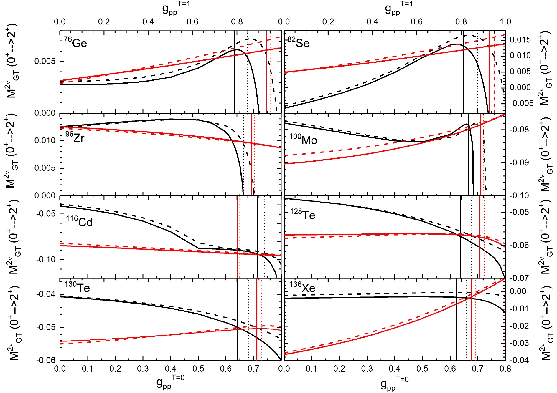
Figure 1. (color online) Dependence of NMEs for
$ 2\nu\beta\beta $ to first$ 2^+ $ excited states on the strength of the isovector ($ g_{pp}^{T = 1} $ ) and isoscalar ($ g_{pp}^{T = 0} $ ) ppresidual interactions. Here, the solid lines are for the larger model space, and dashed lines for the smaller one, as indicated in the text. The red curves are for the isovector dependence, and black ones for the isoscalar. The upper x-axes of each panel are for $ g_{pp}^{T = 1} $ and lower ones for$ g_{pp}^{T = 0} $ ; they have different scales. The vertical lines are for the fitted$ g_{pp} $ 's with unquenched$ g_A $ with line styles following those of the curves.The dependence of the NMEs for the decay to the excited states on the isoscalar pp channel (black curves in Fig. 1, where we keep
$ g_{pp}^{T = 1} $ constant with the fitted value mentioned above) is much more complex than that for the decay to the ground states [15]. These curves suggest that when$ g_{pp}^{T = 0} $ approaches the values where the QRPA equations collapse, the corresponding NME will drop rapidly to$ -\infty $ ; this is similar to the decay to the ground states (see e.g., [15]). Besides, for 128Te, 130Te, and 136Xe, we find similar trends for the$ g_{pp}^{T = 0} $ dependence of the decays to the excited and ground states; this may suggest a commonality in the structures of their$ 2^+ $ states and ground states. For 116Cd, a similar decreasing trend of the curve is observed, except there is a deceleration in this decrease after a specific point. The remaining nuclei show diversities for the$ g_{pp}^{T = 0} $ dependence. 76Ge and 82Se experience a smooth accelerating increase before a sudden decrease near the QRPA collapse. Meanwhile, 96Zr undergoes a mild increase before a rapid drop in the NME. Moreover, 100Mo combines the behaviors of the above nuclei. On the other hand, at$ g_{pp}^{T = 0} = 0 $ , some NMEs are positive and other negative. There is actually a phase uncertainty in the NMEs because the measurements can determine only their absolute values, and in this study, we use the phase convention that forces the values of the NMEs near the QRPA collapse to be$ -\infty $ to match the behavior of the decays to the ground states for the sake of comparison.Opposite to the case for isoscalar interactions, the NMEs change almost monotonically when
$ g_{pp}^{T = 1} $ , and the isovector pp interaction strength changes (red curves). Effectively, the study of the double beta decay is concerned more about the absolute NME rather than the actual NME, because the half-lives depend on the square of the NME. With this respect, we find that some nuclei have a reduced decay strength with increasing$ g_{pp}^{T = 1} $ , whereas others, such as 76Ge, achieve an enhanced strength. As for the magnitude of the changes by varying$ g_{pp}^{T = 1} $ , it is usually smaller than that of$ g_{pp}^{T = 0} $ , except for 136Xe. For the isovector interaction, sharp drops in the NMEs are not observed. This is because the collapse of the QRPA occurs with$ g_{pp}^{T = 1} $ much larger than the realistic values.Figure 1 shows that the size of the model space does not affect the evolving behavior of the NMEs, although it does change their actual values for specific
$ g_{pp} $ 's. Typically, for a smaller model space, larger fitted$ g_{pp} $ values are expected. However, for most cases, the resulting NMEs do not change significantly. This suggests that the model space truncation affects the NMEs of the decays to the ground states and excited states in the same way. Thus, the results with the SMSp and the LMSp differ only by several percent; however, for the nuclei whose NMEs at realistic$ g_{pp} $ values are near zero (136Xe), the truncation of the model space may lead to large relative changes in the NMEs.Our results can be compared to the results obtained from other QRPA calculations [9, 18], where
$ g_{pp}^{T = 1} $ and$ g_{pp}^{T = 0} $ have not been separated and smaller model spaces are used. Because the evolving trend of$ g_{pp}^{T = 1} $ is monotonic, the combined evolving trends of$ g_{pp} $ are more close to that of$ g_{pp}^{T = 0} $ . We find that we have similar trends as in other calculations, but we have different NME values. Meanwhile, the different calculations deviate from each other, and a large discrepancy exists between them. If we consider calculations from other approaches, the discrepancies could be further magnified. These discrepancies can only be solved by measurements. From Fig. 1, we learn that the treatment of the isospin symmetry restoration ($ g_{pp}^{T = 0}\ne g_{pp}^{T = 1} $ ) can alter the final NMEs within several percent by most nuclei, except 136Xe. Because the final NMEs for 136Xe cross zero in the relavant$ g_{pp} $ region, the old isospin violation treatment will provide a fairly large NME.To understand the behavior of the NME dependence on
$ g_{pp} $ , one can examine the running sum, which shows how the low- and high-lying states contribute. We plot in Fig. 2 two typical cases, 76Ge and 130Te, which we discussed above. At first, the running sum shows a more complex structure than the$ \beta\beta $ -decay to the ground states [21, 22]. According to [22], low-lying states contribute mostly positively and contributions from high-lying states may enhance or reduce the total NMEs according to the values of$ g_{pp} $ . However, in the calculations of the decay to$ 2^+_1 $ , this is quite different; the high-lying contributions are largely suppressed, and the effect starts to appear only near the collapse of the QRPA. In the realistic$ g_{pp} $ region, most of the contributions are from the low-lying transitions, and they may add or cancel each other from case to case.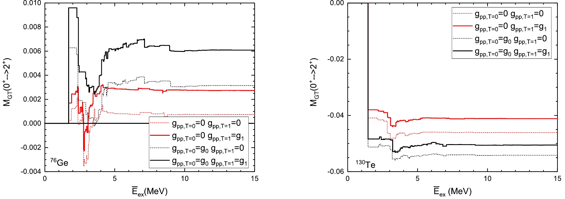
Figure 2. (color online) Running sum of
$ 2\nu\beta\beta $ to$ 2^+_1 $ for 76Ge and 130Te. Here,$ g_{0} $ and$ g_{1} $ are the fitted$ g_{pp} $ values for T = 0 channel and T = 1 channel, respectively, with unquneched$ g_A $ .The isovector pp interactions do not change the basic structure of the running sums; however, they slightly change the magnitude of each transition; this can be seen by comparing the solid and dashed curves. For each nuclei, we can always find the corresponding transitions between the cases with and without the isovector pp interactions. These transitions are with similar energies but differ by the absolute magnitude of the transition strength. For both low- and high-lying strengths, we can also find an increasing strength with the isovector strength.
The effect of the pp interactions in the isoscalar channel on the NMEs can be acquired by comparing the red and black curves. When
$ g_{pp}^{T = 0} $ is zero, barely no high-lying state contributions are observed; with large$ g_{pp}^{T = 0} $ , we see moderate reductions from the high-lying states near 10 MeV (the proposed GT resonance (GTR) region) for 76Ge. This reduction from the high-lying states becomes drastic near the QRPA collapse in our calculation (for 130Te, this effect is not shown in the sum rule because the fitted$ g_{pp}^{T = 0} $ is far away from the collapse, and near collapse, we could observe a reduction around the GTR energies). This leads to the drastic decrease in the NMEs at very large$ g_{pp}^{T = 0} $ in Fig. 1. From Fig. 2, we can also understand the different behaviors of the NME's$ g_{pp}^{T = 0} $ dependence of various nuclei. For example, for 76Ge, the low-lying strengths strongly cancel each other, whereas the positive strengths grow faster than the negative ones with increasing$ g_{pp}^{T = 0} $ , which causes the accelerated increase until the reduction from the high-lying states mentioned above dominates the NME. This contradicts the 130Te case where all the major strengths are negative and add together, and so, no increase in the strength is observed; the contribution from the high-lying states (not shown in the graph) further reduces the results. In the low-lying energy region, the isoscalar pp interactions change not only the strength of each state but also the structure of the running sum; this produces the complex evolution of the NME. -
PSFs of the decay to the
$ 2^+_1 $ state have been addressed in several publications [3, 23, 24]. In this study, we calculate the PSF with the numerical electron wavefunctions from the numerical package, RADIAL [16]; to avoid complication, we assume the electron wavefunction is constant inside the nucleus. This allows a separation of the calculations of the NMEs and the PSFs, as discussed above. We use a uniformly distributed electric charge in the nuclei to take into consideration the nuclear finite size [17], and the charge radius is taken to be the empirical nuclear radius,$ R = 1.2A^{1/3} $ fm. We neglect the screening effect of the atomic electrons. Their effects are analyzed in studies such as [24]. To separate the nuclear and lepton parts, one uses the average excitation energies,$ \tilde{A} $ , in the phase space calculations (see Eq. (2)). There is always an arbitrariness in the choice for$ \tilde{A} $ in such a formalism. To estimate the possible error due to this choice, we plot the dependence of this PSF on$ \tilde{A} $ for 116Cd in Fig. 3, where the curve starts at the lowest possible average energy ($ \tilde{A}_{\rm SSD} $ ) that is experimentally known. Here, SSD is the abbreviation of “single-state dominance”, and this single state usually refers to the first$ 1^+ $ state of the intermediate states. As one can see, the PSF reaches its largest value at the point of$ \tilde{A}_{\rm SSD} $ , then it rapidly drops to a nearly constant value at the average energy of approximately 5 MeV, and after that it barely changes. 116Cd decays to the excited state of 116Sn. The value changes about 30%, which is close to the case of the decay to the ground states [17].
Figure 3. (color online) Phase space factor for
$ 2\nu\beta\beta $ to$ 2^+_1 $ of 116Cd as a function of average excitation energy$ \tilde{A} $ , where$ \tilde{A}_{\rm SSD} $ corresponds to the single-state dominance case in which the average excitation energy of the intermediate nucleus is 0, and for$ \tilde{A}_{\rm GTR} $ , the average excitation energy of the intermediate nucleus is taken to be the GTR energy from [17].For the PSF calculations, there are usually two kinds of choices for
$ \tilde{A} $ , SSD mentioned above and high-lying state dominance (HSD). Here, a high-lying state usually refers to the strong GTR, which is observed in charge-exchange experiments and its position can be obtained from systematics [17]. For the optimal choices of$ \tilde{A} $ , one could resort to nuclear structure data. Our analysis above about the running sum suggests that for the decays to$ 2^+ $ , the low-energy states, especially the first states, make the largest contribution to the NME; therefore we choose$ \tilde{A}_{\rm SSD} $ in this study. These calculated PSFs are tabulated in Table 1. We have also tabulated the previous results from Ref. [3], which uses the HSD ($ \tilde{A} = 10 $ MeV for all the nuclei) for the estimation of the PSF, and we present also our calculated PSFs from the HSD for the sake of comparison. By comparing our results with those in Ref. [3], we find that the two sets of results are generally within the same order of magnitude. The deviations between the current calculations and the previous one are within a factor of 2; our current calculations with numerical electron wavefunctions yield smaller PSFs, and the reductions vary from 10%–40%. The reason for such an overestimation from the previous study is that they use the constant electron wavefunctions with the values at the center of the nuclei, whereas we use the values at the surface. Such a choice at the nuclear surface also comes from the implications of nuclear structure calculations, such as those for single-$ \beta $ decay in [25] and for$ \beta\beta $ -decay in [26]. As shown in Fig. 3, the SSD PSFs correspond to larger PSFs, and therefore, short half-lives. The errors from the choice of$ \tilde{A} $ for the PSF depends on the Q values as well as the$ 1^+ $ intermediate states energies. The reduction for the HSD to SSD can be as large as 60% for certain nuclei; but it can also be small, such as for 128Te with a much smaller PSF.$t^{2\nu,{\rm exp}}_{1/2}(0^+_1)$ /yr [6]

Q/MeV $G^{2\nu}_{2^+_1}$ /(yr−1MeV6)

$M^{2\nu}_{2^+_1}$ /MeV-3

$t^{2\nu,{\rm theo}}_{1/2}(2^+_1)$ /yr

$t^{2\nu,{\rm exp}}_{1/2}(2^+_1)$ /yr [5]

$Br(2^+_1)$ 

[3] HSD SSD 76Ge $1.65^{+0.14}_{-0.12}\times 10^{21}$ 

1.480 8.620 $\times 10^{-24}$ 

7.599 $\times10^{-24}$ 

1.053 $\times10^{-23}$ 

6.08 $\times 10^{-3}$ 

3.33 $\times 10^{27}$ 

$>1.6\times 10^{23}$ 

5.0 $\times 10^{-7}$ 

82Se $(9.2 \pm 0.7)\times 10^{19}$ 

2.219 1.569 $\times 10^{-21}$ 

1.354 $\times 10^{-21}$ 

3.408 $\times 10^{-21}$ 

1.31 $\times 10^{-2}$ 

1.96 $\times 10^{24}$ 

$>1.0\times 10^{22}$ 

4.7 $\times 10^{-5}$ 

96Zr $(2.3 \pm 0.2)\times 10^{19}$ 

2.572 − 1.407 $\times 10^{-20}$ 

1.935 $\times 10^{-20}$ 

1.16 $\times 10^{-2}$ 

4.67 $\times 10^{23}$ 

$>7.9\times 10^{19}$ 

4.9 $\times 10^{-5}$ 

100Mo $(7.1 \pm 0.4)\times 10^{18}$ 

2.495 1.382 $\times 10^{-20}$ 

1.127 $\times 10^{-20}$ 

2.989 $\times 10^{-20}$ 

−7.83 $\times 10^{-2}$ 

6.63 $\times 10^{21}$ 

$>2.5\times 10^{21}$ 

1.1 $\times 10^{-3}$ 

116Cd $(2.87 \pm 0.13)\times 10^{19}$ 

1.520 − 4.120 $\times 10^{-23}$ 

6.156 $\times 10^{-23}$ 

−9.05 $\times 10^{-2}$ 

2.41 $\times 10^{24}$ 

$>2.3\times 10^{21}$ 

1.2 $\times 10^{-5}$ 

128Te $(2.0 \pm 0.3)\times 10^{24}$ 

0.423 2.350 $\times 10^{-29}$ 

1.779 $\times 10^{-29}$ 

1.813 $\times 10^{-29}$ 

−5.72 $\times 10^{-2}$ 

2.05 $\times 10^{31}$ 

− 9.8 $\times 10^{-8}$ 

130Te $(6.9 \pm 1.3)\times 10^{20}$ 

1.991 2.119 $\times 10^{-21}$ 

1.581 $\times 10^{-21}$ 

2.713 $\times 10^{-21}$ 

-5.00 $\times 10^{-2}$ 

1.79 $\times 10^{23}$ 

$>2.8\times 10^{21}$ 

3.9 $\times 10^{-3}$ 

136Xe $(2.19 \pm 0.06)\times 10^{21}$ 

1.639 2.659 $\times 10^{-22}$ 

1.755 $\times 10^{-22}$ 

5.179 $\times 10^{-22}$ 

-3.04 $\times 10^{-3}$ 

2.54 $\times 10^{26}$ 

$>4.6\times 10^{23}$ 

8.6 $\times 10^{-6} $ 

Table 1. Calculated phase space factors from [3] and this study, and the decay half-lives for the
$\beta\beta$ -decay to the first$2^+$ states from this study, where the queching factor,$g_A = 0.75 g_{A0}$ , is used. The experimental half-lives or half-life limits of$2\nu\beta\beta$ to the ground states and first$2^+$ states are tabulated as well. Here,$Br(2^+)$ is the branch ratio of the decay to$2^+$ to the overall$2\nu\beta\beta$ .The half-life of the decay to the first
$ 2^+ $ can be obtained by combining the calculated NME and PSF. Here, for the 8 nuclei involved, the largest NME comes from 116Cd and the smallest comes from 136Xe, and the difference is more than a factor of 10. The difference among the PSFs is much larger. Three orders of magnitude deviations are observed for most nuclei, mostly owing to their different Q values, and an extremely small PSF is found for 128Te, which has a small Q value.The half-lives of these nuclei cross a large region, from
$ \sim 10^{22} $ to$ \sim 10^{32} $ years. 100Mo has the shortest half-life for both the$ 2\nu\beta\beta $ -decay to the ground and$ 2^{+}_1 $ states, and it also has a reasonably large decay branching ratio. This suggests its$ \beta\beta $ -decay to the$ 2^+_1 $ states has the largest potential to be detected. In comparison, 128Te with a half-life of$ 10^{32} $ years seems impossible to be detected. The same is the case for 76Ge and 136Xe. These three nuclei have extremely low branching ratios of the decay to the$ 2^+ $ to the overall$ \beta\beta $ -decays either owing to the small PSF (128Te) or small NME (76Ge and 136Xe). 96Zr, 130Te, and 100Mo are promising candidates for future experiments. Especially for 100Mo, the current experimental limit is close to the predicted half-life with less than one order of magnitude difference. With future improvements in the experiments, it is perhaps possible to observe the special$ 2^+_1 $ mode of this nucleus, because it is also the first nucleus for which the decay to the first$ 0^+ $ excited was observed. For the other nuclei, observations of the$ \beta\beta $ -decay to$ 2^+_1 $ can be quite difficult owing to their long half-lives and small branching ratios. -
In this study, we calculated the NMEs and PSFs of
$ 2\nu\beta\beta $ to the first$ 2^+ $ states for eight nuclei with partially restored isospin symmetry. We studied the NME dependence on the isovector and isoscalar pp residual interaction strengths. Finally, we predicted the half-lives and branching ratios of these decays to excited states. However, further investigation on the effect of anharmonicity of the$ 2^+ $ phonon to the decay is needed.We would like to thank Prof. F. Šimkovic for useful discussions and help on the code.
2νββ-decay to first 2+ states with partial isospin symmetry restoration from spherical QRPA calculations
- Received Date: 2020-03-02
- Available Online: 2020-08-01
Abstract: Using partially restored isospin symmetry, we calculate the nuclear matrix elements for a special decay mode of a two-neutrino double beta decay – the decay to the first 2+ excited states. Employing the realistic CD–Bonn nuclear force, we analyze the dependence of the nuclear matrix elements on the isovector and isoscalar parts of proton–neutron particle–particle interactions. The dependence on the different nuclear matrix elements is observed, and the results are explained. We also provide the phase space factors using numerical electron wavefunctions and properly chosen excitation energies. Finally, we present our results for the half-lives of this decay mode for different nuclei.


 DownLoad: