


 Abstract
 HTML
HTML Reference
 Related
 PDF
PDF


-
The anomalous transport of chiral magnetic effect (CME) has gained significant attention over the past few years [1, 2]. If the local parity odd domain is present in the quark-gluon plasma produced in heavy ion collisions, CME leads to charge separation along the magnetic field generated in off-central collisions:
$ { j}_e = \sum\limits_f\frac{N_cq_f^2}{2\pi^2}{\mu}_A{ B}, $

(1) where the chiral imbalance,
$ {\mu}_A $ , characterizes local parity violation. This offers the possibility of detecting local parity violation in quantum chromodynamics (QCD). Charge separation has been actively sought experimentally [3-5]. However, we are still far from consensus on the status of CME, largely due to the difficulty in determining CME both experimentally and theoretically; see [6-9] for recent reviews. Experimentally, charge separation needs to be measured through charged hadron correlation on an event-by-event basis. Unfortunately, charged hadron correlation is dominated by flow-related background with various possible origins [10-12]. Various observables and experimental techniques have been proposed and implemented to exclude flow-related background [13-16]. In addition, STAR collaboration proposes to search for CME in isobar collisions [17]. Since isobars have the same atomic number but different proton numbers, the corresponding collisions are supposed to generate the same flow background, but different magnetic field, and thus, different charge separation. This can unambiguously distinguish the CME contribution.Theoretically describing CME is also difficult. Both
$ {\mu}_A $ and B contain large uncertainties. Their peak values are known to be set by the axial charge production in glasma phase [18, 19] and the moving charge of spectators [20], respectively. However, their further evolution is model dependent. Different theoretical frameworks, such as anomalous viscous fluid dynamics (AVFD) [21-24], chiral kinetic theory [25-27], and the multiphase transport model [28, 29], have been employed to study the time evolution of axial/vector charges. All these frameworks treat axial charge as an approximately conserved quantity in the absence of parallel electric and magnetic fields. However, axial charges are not conserved, due to gluon dynamics. In fact, it is the same origin for the initial axial charge. In [30], the authors incorporated fluctuation and dissipation of axial charge in the framework of stochastic hydrodynamics. We found that independent of the initial conditions, the variance of axial charge always approaches the thermodynamic limit after sufficient time, due to the interplay of fluctuation and dissipation. In [30], we used the thermodynamic limit for the axial charge to model CME. While being model-independent, the study missed an important fact: most charge separation occurs at early stages of quark-gluon plasma formation, when$ {\mu}_A $ and B have not decayed appreciably. This study aims to incorporate the initial axial charge and investigate the coupled dynamics of axial and vector charge. In particular, we make predictions for the CME contribution to isobar collisions.This paper is organized as follows. In Sec. 2, we generalize the stochastic hydrodynamics framework to include axial and vector charge, which are coupled through anomalous effects in the presence of the magnetic field. Subsequently, we will justify the claim that for phenomenologically relevant magnetic fields, the back-reaction of vector charge to axial charge is negligible. In Sec. 3, we derive axial charge evolution with a non-vanishing initial value. The obtained axial charge is used to calculate charge separation. We make predictions for CME in isobar collisions, using AuAu collisions as a reference. We conclude and discuss directions for future work in Sec. 4.
-
The stochastic hydrodynamic equations for axial charge in the absence of magnetic field are given in [30]. In a magnetic field, axial charge couples to vector charge through the chiral magnetic effect and chiral separation effect (CSE). The full stochastic hydrodynamic equations for axial and vector charges are
$ \left\{\begin{split} \nabla_{\mu} J_A^{\mu} &= -\frac{n_A}{\tau_{{\rm{CS}}}}-2{\xi}_q \\ J_A^{\mu} &= n_A u^{\mu}+{\lambda} n_V eB^{\mu}-{\sigma} TP^{{\mu}{\nu}}\nabla_{\nu}\left( {\frac{n_A}{\chi_A T}} \right)+{\xi}_A^{\mu}, \end{split}\right. $

(2) and
$ \left\{\begin{split} \nabla_{\mu} J_V^{\mu}& = 0 \\ J_V^{\mu}& = n_V u^{\mu}+{\lambda} n_A eB^{\mu}-{\sigma} TP^{{\mu}{\nu}}\nabla_{\nu}\left( {\frac{n_V}{\chi_V T}} \right)+{\xi}_V^{\mu}. \end{split}\right. $

(3) $ n_A $ and$ n_V $ are axial and vector charge density, respectively. The axial current is not conserved, due to the topological configuration of gluons. This leads to the dissipative term,$ \sim\frac{n_A}{{\tau}_{\rm{CS}}} $ , and fluctuating noise term,$ \sim{\xi}_q $ . The constitutive equations for axial and vector current consist of a co-moving term, an anomalous mixing term, a diffusive term, and a thermal noise term.$ u^{\mu} $ is the fluid velocity, which defines the projection operator,$ P^{{\mu}{\nu}} = g^{{\mu}{\nu}}+u^{\mu} u^{\nu} $ and the magnetic field in the fluid cell,$B^{\mu} = -\dfrac{1}{2}\dfrac{{\epsilon}^{{\mu}{\nu}{\alpha}{\beta}}}{\sqrt{-g}}F_{{\alpha}{\beta}}u_{\nu}$ .$ {\xi}_A $ ,$ {\xi}_V $ , and$ {\xi}_q $ are considered as Gaussian white noises:$ \begin{split} &\left\langle {{\xi}_A^{\mu}(x){\xi}_A^{\nu}(x')} \right\rangle = P^{{\mu}{\nu}}2{\sigma}_AT\frac{ \,{\rm{d}}^4(x-x')}{\sqrt{-g}}, \\ &\left\langle {{\xi}_V^{\mu}(x){\xi}_V^{\nu}(x')} \right\rangle = P^{{\mu}{\nu}}2{\sigma}_VT\frac{ \,{\rm{d}}^4(x-x')}{\sqrt{-g}}, \\ &\left\langle {{\xi}_q(x){\xi}_q^{\nu}(x')} \right\rangle = {\Gamma}_{\rm{CS}}\frac{ \,{\rm{d}}^4(x-x')}{\sqrt{-g}}, \\ &\left\langle {{\xi}_A^{\mu}(x){\xi}_q(x')} \right\rangle = \left\langle {{\xi}_V^{\nu}(x){\xi}_q(x')} \right\rangle = 0, \end{split} $

(4) with
$ {\Gamma}_{\rm{CS}} $ being the Chern-Simon diffusion constant characterizing the magnitude of topological fluctuation.For application to CME in heavy ion collisions, we fix the parameters as follows. We use the free theory limit for axial and vector charge susceptibilities,
$ {\chi_A = \chi_V = \chi} = N_fN_cT^2/3 $ . The coefficient of the mixing term,$ {\lambda} $ , is determined by the chiral magnetic/separation effect as$ {\lambda} = \dfrac{1}{\chi}\dfrac{N_c}{2\pi^2} $ . The quark mass effect on CSE can be neglected [31]. For three flavours, we have$ {\chi = 3T^2} $ and$ {\lambda} = \dfrac {1}{2\pi^2T^2} $ .$ {\Gamma}_{\rm{CS}} $ is the Chern-Simon diffusion constant, obtained from the extrapolated weak coupling results:$ {\Gamma}_{\rm{CS}} = 30{\alpha}_s^4T^4 $ [32] with$ {\alpha}_s = 0.3 $ . The relaxation time of the axial charge,$ {\tau}_{\rm{CS}} $ , is fixed by the Einstein relation:$ {\tau}_{\rm{CS}} = {\dfrac{\chi T}{2{\Gamma}_{\rm{CS}}}} $ .$ {\sigma}_A $ and$ {\sigma}_V $ are the conductivities for the axial and vector currents, and are not required in our analysis.The axial/vector charge is treated as a perturbation in the background hydrodynamic flow. We consider heavy ion collisions at the top RHIC collision energy,
$ \sqrt{s_{{NN}}} = {200\; {\rm{GeV}}} $ , using Bjorken flow as the background. In the Milne coordinates$ (\tau, \eta, x, y) $ , the fluid velocity is$ u^{\mu} = (1,0,0,0) $ . We can show that the total axial charge is conserved up to a mixing term and the topological fluctuation-induced terms. To do so, we substitute the constitutive equation into the conservation equation in (2) and integrate over the volume,$ \int{\tau} {\rm d}{\eta} {\rm d}^2x_\perp = \int\sqrt{-g}{\rm d}{\eta} {\rm d}^2x_\perp $ . The identity,$ \nabla_{\mu} V^{\mu} = \dfrac{1}{\sqrt{-g}}\partial_{\mu}\left( {\sqrt{-g}V^{\mu}} \right) $ , dropping the boundary terms, yields$ \begin{split} \int {\rm d}{\eta} {\rm d}^2x_\perp\left( {\partial_{\tau}\left( {{\tau} n_A} \right)-\partial_{\tau}\left( {{\sigma}_ATP^{{\tau}{\nu}}\nabla_{\nu}\left( {\frac{n_A}{{ \chi T}}} \right)} \right)+\partial_{\tau}\left( {{\tau}{\xi}_A^{\tau}} \right)} \right) = \int {\rm d}{\eta} {\rm d}^2x_\perp\left( {-\frac{{\tau} n_A}{{\tau}_{\rm{CS}}}-2{\tau}{\xi}_q} \right).\end{split} $

(5) Note that
$ P^{{\mu}{\nu}}u_{\nu} = 0 $ and$ {\xi}_A^{\mu}{\xi}_A^{\nu}\sim P^{{\mu}{\nu}} $ . Thus,$ P^{{\tau}{\nu}} = 0 $ and$ {\xi}_A^{\tau} = 0 $ . We then arrive at$ \begin{align} \partial_{\tau} N_A = -\frac{N_A}{{\tau}_{\rm{CS}}}-\int {\rm d}{\eta} {\rm d}^2x_\perp2{\tau}{\xi}_q, \end{align} $

(6) with
$ N_A = \int{\tau} {\rm d}{\eta} {\rm d}^2x_\perp $ . The absence of the diffusive term, thermal noise term, and mixing term is consistent with the fact that these terms only lead to the redistribution of axial charge. The counterpart for the vector charge is simpler:$ \partial_{\tau} N_V = 0 $ , because vector charge is strictly conserved. -
We assume that the initial axial charge created by the chromo flux tube is homogeneous in the transverse plane. The boost-invariant Bjorken expansion maintains a homogeneous distribution in the longitudinal direction. The homogeneous axial charge leads to charge separation via CME. This simplified picture is modified by three effects: diffusion, thermal noise, and CSE. The thermal noise and diffusion correspond to the fluctuation and dissipation of charge, which bring the charge to equilibrium. The CSE is not balanced by other effects. We will now show that its effect is sub-leading.
Let us compare the axial charge,
$ n_A $ , and CSE modification,$ \sim{\lambda} B n_V $ . Since$ \chi_A = \chi_V $ , it is equivalent to comparing$ {\mu}_A $ and$ {\lambda} B{\mu}_V $ . Since B drops quickly with time, the CSE effect is maximized at initial time. We estimate the initial$ n_A $ following [21] as$ \begin{align} \sqrt{\langle n_A({\tau}_0)^2\rangle}\simeq \frac{Q_s^4(\pi {\rho}_{\rm{tube}}^2{\tau}_0)\sqrt{N_{{\rm{coll}}}}}{16\pi^2S_\perp}, \end{align} $

(7) where
$ Q_s $ is the saturation scale and$ {\rho}_{\rm{tube}}\simeq {1\; {\rm{fm}}} $ is the width of the flux tube.$ {\tau}_0 $ is the initial proper time. For AuAu collisions, we employ$ Q_s\simeq {1\; {\rm{GeV}}} $ and$ {\tau}_0 = {0.6\; {\rm{fm}}} $ . The number of binary collisions,$ N_{{\rm{coll}}} $ , and transverse overlap area,$ S_\perp $ , are calculated using a Monte Carlo Glauber model [33-36] with the centrality dependence listed in Table 1.centrality 0-5% 5%-10% 10%-20% 20%-30% 30%-40% 40%-50% 50%-60% 60%-70% 70%-80% Au $ N_{\rm{coll}} $ 

1049.8 843.9 594.8 369.1 217.4 121.6 62.2 29.2 12.7 $ S_\perp/{\rm{fm}}^2 $ 

147.9 128.9 106.1 83.0 64.8 49.7 36.6 25.5 16.2 $ L_\perp/{\rm{fm}} $ 

13.2 11.9 10.3 8.6 7.3 6.1 5.0 4.1 3.1 Ru $ N_{\rm{coll}} $ 

387.5 316.3 228.9 146.6 90.9 53.6 30.0 15.8 8.1 $ S_\perp/{\rm{fm}}^2 $ 

92.5 81.6 67.8 53.8 42.3 32.8 24.7 17.6 12.1 $ L_\perp/{\rm{fm}} $ 

10.5 9.5 8.3 7.0 6.0 5.1 4.3 3.5 2.9 Zr $ N_{\rm{coll}} $ 

395.6 322.5 232.1 149.0 91.8 54.0 30.1 15.7 8.0 $ S_\perp/{\rm{fm}}^2 $ 

91.3 80.5 67.0 53.1 41.8 32.5 24.4 17.4 11.9 $ L_\perp/{\rm{fm}} $ 

10.4 9.4 8.2 7.0 6.0 5.0 4.2 3.5 2.9 Table 1. Geometrical quantities from the MC-Glauber model for Au, Ru and Zr.
$ N_{{\rm{coll}}} $ ,$ S_\perp $ , and$ L_\perp $ are the number of binary collisions, transverse overlap area, and width of the participants' region along the cross-line between the transverse and reaction planes, respectively.$ S_\perp $ is considered to be the projection of the nucleon-nucleon cross-section$ {\sigma}_{{NN}} $ onto the transverse plane [37], and$ L_\perp $ is calculated through the same algorithm as$ S_\perp $ .$ 10k $ events are run to generate the data. Averages are found using the impact parameter b as the weight factor.The initial temperature is taken as
$ T_0 = {350\; {\rm{MeV}}} $ . These combined give$ {\mu}_A\simeq {36\; {\rm{MeV}}} $ with weak centrality dependence. In contrast,$ {\mu}_V $ is estimated from [38]$ {\mu}_B(s)\simeq\frac{a}{1+\sqrt{s}/b}, $

(8) with
$ a\simeq {1.27\; {\rm{GeV}}} $ and$ b\simeq {4.3\; {\rm{GeV}}} $ at$ \sqrt{s_{{NN}}} = {200\; {\rm{GeV}}} $ ,$ {\mu}_B\simeq {27\; {\rm{MeV}}} $ , corresponding to$ {\mu}_V\simeq {9\; {\rm{MeV}}} $ . Taking the peak value of$ B\simeq 10m_\pi^2 $ , we determine that$ {\lambda} eB{\mu}_V/{\mu}_A\simeq $ 3%. Since the magnetic field decays rapidly with time, a more realistic estimation method for the back-reaction is to use the time-averaged magentic field. Assuming the following functional form of magnetic field [39, 40],$ eB({\tau}) = \frac{eB_0}{1+({\tau}/{\tau}_B)^2}, $

(9) and averaging between initial time
$ {\tau}_0 = {0.6\; {\rm{fm}}} $ and freeze-out time$ {\tau} = {7\; {\rm{fm}}} $ , we obtain$ {\lambda} {eB}_{avg}{\mu}_V/{\mu}_A\simeq $ 1% for$ {\tau}_B = {2\; {\rm{fm}}} $ and$ {\lambda} {eB}_{avg}{\mu}_V/{\mu}_A\simeq $ 0.4% for$ {\tau}_B = {1\; {\rm{fm}}} $ . Therefore, we can safely neglect the CSE effect on axial charge redistribution. Similar analysis shows that the same is true for the isobar collisions. -
Since the back-reaction from vector charge is negligible, we can trace the evolution of the total axial charge and use it to determine the average
$ {\mu}_A $ for CME phenomenology. In [30], we derived the hydrodynamic evolution of the total axial charge with an initial value. It is given by$\begin{split} \langle N_A({\tau})^2\rangle =& \langle N_A({\tau}_0)^2\rangle {\rm e}^{3\left( {1-\left( {\frac{{\tau}}{{\tau}_0}} \right)^{2/3}} \right)\left( {\frac{{\tau}_0}{{\tau}_{{\rm{CS}}0}}} \right)}\\&+\int \,{\rm{d}}{\eta} \,{\rm{d}}^2x_\perp 2{\Gamma}_0{\tau}_0{\tau}_{{\rm{CS}}0}\left( {1-{\rm e}^{3\left( {1-\left( {\frac{{\tau}}{{\tau}_0}} \right)^{2/3}} \right)\left( {\frac{{\tau}_0}{{\tau}_{{\rm{CS}}0}}} \right)}} \right). \end{split}$

(10) The initial conditions for the AuAu collisions at
$ \sqrt{s_{{NN}}} = {200\; {\rm{GeV}}} $ has been discussed in the previous subsection. The counterpart for the isobars scales accordingly. We adopt the scaling of$ Q_s $ with the system size from [41] and the initial time for Bjorken hydrodynamics from [42]. The freeze-out time is determined by the same freeze-out temperature,$ T_f = {154\; {\rm{MeV}}} $ . We list the scalings as follows:$ \begin{split}& Q_s\sim A^{\frac16}, \quad T_0\sim Q_s\sim A^{\frac16}, \\ &{\tau}_0\sim 1/{Q_s} \sim A^{-\frac16},\quad {\tau}_f\sim A^{\frac13}. \end{split} $

(11) The axial chemical potential is calculated using the average axial charge
$ {\mu}_A({\tau}) = \frac{\sqrt{\langle n_A({\tau})^2\rangle}}{{\chi({\tau})}} = \frac{\sqrt{\langle N_A({\tau})^2\rangle}}{V({\tau})\ {\chi({\tau})}}, $

(12) with
$ V({\tau}) = S_\perp{\tau}{\Delta}{\eta} $ being the total volume. The rapidity span is taken to be$ |{\eta}|<2 $ with$ {\Delta}{\eta} = 4 $ . Consequently, the axial chemical potential is determined as$ \begin{split} {\mu}_A({\tau}) = {\mu}_{A0}\left(\frac{{\tau}}{{\tau}_0}\right)^{-\frac13} \sqrt{{\rm e}^{3\left( {1-\left( {\frac{{\tau}}{{\tau}_0}} \right)^{2/3}} \right)\left( {\frac{{\tau}_0}{{\tau}_{{\rm{CS}}0}}} \right)}+\frac{3T_0^3}{{\tau}_0\ {\Delta}{\eta}\ S_\perp\ n_{A0}^2}\left[1-{\rm e}^{3\left( {1-\left( {\frac{{\tau}}{{\tau}_0}} \right)^{2/3}} \right)\left( {\frac{{\tau}_0}{{\tau}_{{\rm{CS}}0}}} \right)}\right]}, \end{split}$

(13) where the square root factor is a modification to the simple
$ {\tau}^{-1/3} $ dependence when relaxation of axial charge is ignored. The initial axial chemical potential is determined by the initial axial charge density$ n_{A0} $ given in (7) via$ \mu_{A0} = \dfrac{n_{A0}}{\chi_0} = \dfrac{n_{A0}}{3T_0^2} $ .Then, we determine the scalings of the initial axial charge density and chemical potential. From the empirical scaling for the AuAu collisions [33, 37] in the Glauber model,
$ S_\perp \sim N_{\rm{part}}^{\frac23}, \qquad N_{\rm{coll}} \sim N_{\rm{part}}^{\frac43}, $

(14) where
$ N_{\rm{part}} $ is the number of participant nucleons, we have$ S_\perp \sim \sqrt{N_{\rm{coll}}}. $

(15) Thus, from (7) ,
$ n_{A0} $ has only weak centrality dependence. The system size dependence of$ n_{A0} $ and$ {\mu}_{A0} $ can be easily obtained using (11):$ n_{A0} \sim A^{\frac12}, \qquad {\mu}_{A0} \sim A^{\frac16}. $

(16) The centrality dependence of initial chemical potential
$ {\mu}_{A0} $ for Au and isobars are listed in Table 2. A weak centrality dependence is observed for AuAu and a slightly enhanced dependence is observed for Ru and Zu, due to the deviation from the empirical scaling (14). The system size dependence (16) is approximately consistent with Table 2.centrality 0-5% 5%-10% 10%-20% 20%-30% 30%-40% 40%-50% 50%-60% 60%-70% 70%-80% $ {\rm{Au}} $ 

36.11 37.15 37.90 38.14 37.53 36.56 35.49 34.97 36.19 $ {\rm{Ru}} $ 

31.13 31.89 32.63 32.93 32.99 32.63 32.45 33.06 34.55 $ {\rm{Zr}} $ 

31.85 32.62 33.29 33.62 33.51 33.08 32.89 33.35 34.84 Table 2. Centrality dependence of
${\mu}_{A0}\; ({\rm{MeV}})$ . -
Now we can calculate the chiral magnetic current using (1), whose time integral gives the total charge separation
$ Q_e = \int_{{\tau}_0}^{{\tau}_f} \,{\rm{d}}{\tau}\ {\tau} \,{\rm{d}}{\eta} L_\perp\ C_e{\mu}_A\ eB = C_e{\Delta}{\eta}\ L_\perp\int_{{\tau}_0}^{{\tau}_f} \,{\rm{d}}{\tau} \ {\tau} {\mu}_A({\tau})\ eB({\tau}), $

(17) where
$ C_e = \displaystyle\sum_f\dfrac{q_f^2}{e}\dfrac{N_c}{2\pi^2} $ and$ L_\perp $ is the width of the participants' region along the cross-line between the transverse plane and reaction plane, sampled from the MC-Glauber Model, as seen in Table 1. Hence,$ \int {\tau} {\rm d}{\eta} L_\perp $ represents the area that the CME current penetrates in the reaction plane. We integrate it from initial thermalization time$ {\tau}_0 $ to freeze-out time$ {\tau}_f $ , whose values are determined in (11). The effective electric chemical potential is then induced by the total electric charge asymmetry as,$ {\mu}_e({\tau}_f) = \frac{Q_e}{V_f\ \chi_e({\tau}_f)} = \frac{3 L_\perp}{{\pi}^2\ eS_\perp {\tau}_f\ T_f^2} \int_{{\tau}_0}^{{\tau}_f} \,{\rm{d}}{\tau} {\tau} {\mu}_A({\tau})\ eB({\tau}), $

(18) where
$ V_f = S_\perp {\tau}_f {\Delta}{\eta}/2 $ and$ \chi_e({\tau}_f) = \dfrac{1}{3}\displaystyle\sum_fq_f^2N_cTf^2 $ denote the volume of QGP above the reaction plane and the electric charge susceptibility at freeze-out time, respectively.The magnetic field in the lab frame is calculated from the Liénard-Wiechert potentials as
$ e{ B}(t, { r}) = \frac{e^2}{4\pi}\int \,{\rm{d}} { r'}^3 \rho_Z(r')\ \frac{1-{ v}^2}{\left[{ R}^2-({ R}\times { v})^2\right]^{3/2}}{ v}\times { R}\ , $

(19) where
$ { R} = { r}-{ r'}(t) $ is the vector pointing from the proton position$ { r}(t) $ at time t to the position$ { r} $ of the field point.$ { v} $ is the velocity of the protons, chosen to be$ v^2 = 1-{(2m_N/\sqrt{s_{{NN}}})^2} $ , where$ {\sqrt{s_{{NN}}}/2} $ is the energy for each nucleon in the center-of-mass frame and$ m_N $ is the mass of the nucleon. The impact parameter vector is set to be along the x-axis, so that the$ x-z $ plane serves as the reaction plane and$ x-y $ as the transverse plane. We sample the positions of protons in a nucleus in the rest frame by the Woods-Saxon distribution,$ \rho_Z(r')\propto \frac{1}{1+\exp{\left(\dfrac{r'-R_0}a\right)}}, $

(20) where
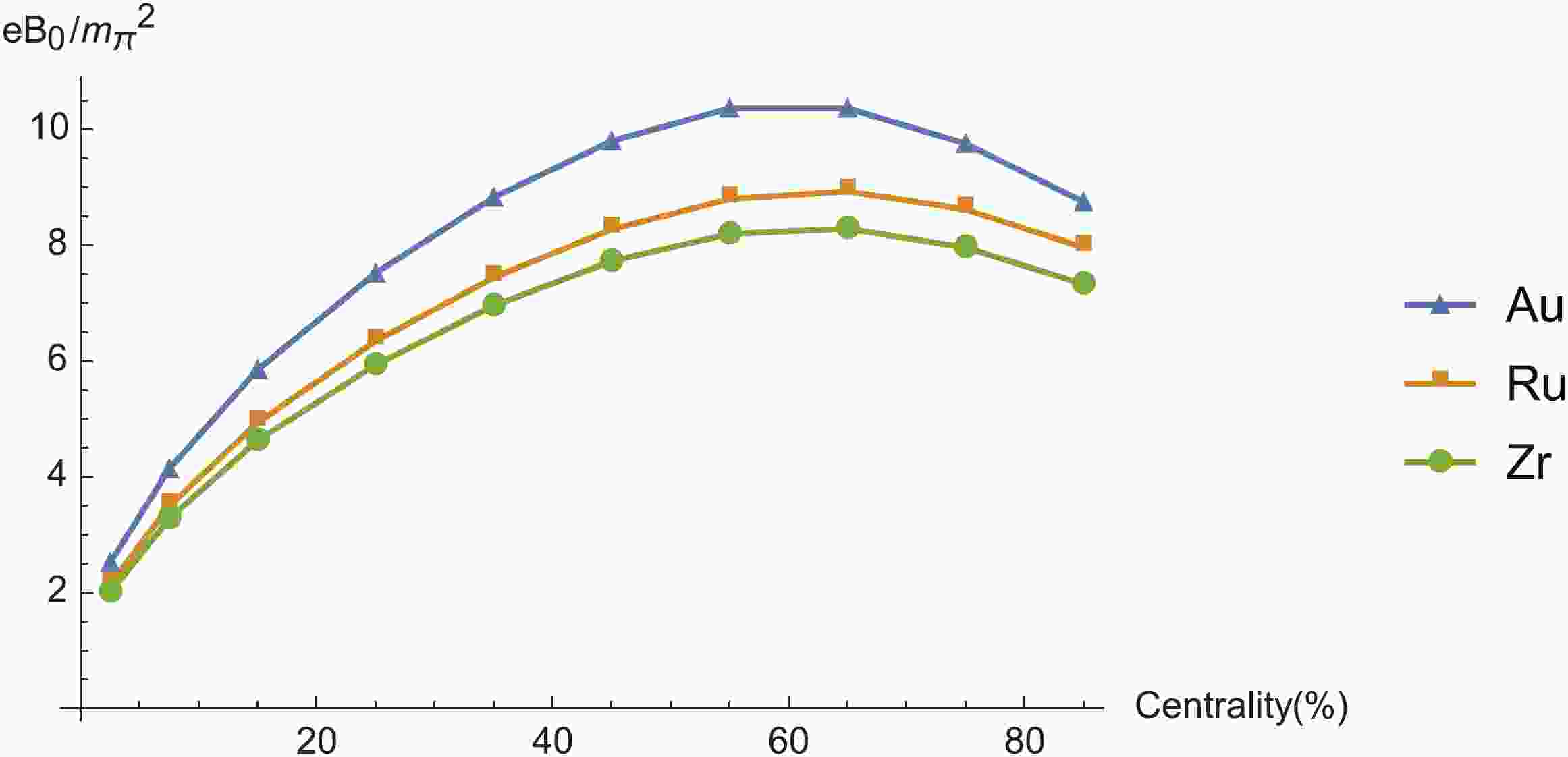
$ R_0 = {6.38\; {\rm{fm}}} $ and$ a = {0.535\; {\rm{fm}}} $ for Au, and$ R_0 = {5.085\; {\rm{fm}}} $ and$ {5.020\; {\rm{fm}}} $ for Ru and Zr, respectively, with$ a = {0.46\; {\rm{fm}}} $ for both isobars. The homogeneity and boost-invariance of the magnetic field is assumed, and the power-decaying form follows from (9) with the peak value$ eB_0 $ set by (19) at$ t = { r} = 0 $ along the y-axis. The dependence on nucleus shape discussed in [43] is not included in our analysis. As a result, the centrality dependence of$ eB_0 $ for Au, Ru, and Zr are shown in Fig. 1. We see that the magnitude of the magnetic field is suggested by the proton numbers of the corresponding nucleus, and that the difference between isobars is indicated as$ \sim $ 10%.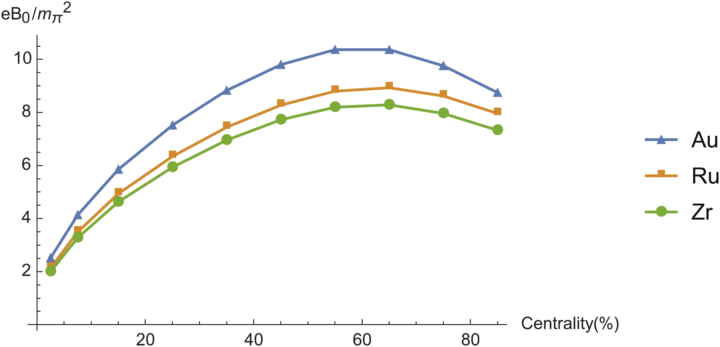
Figure 1. (color online) Centrality dependence of the event-averaged magnetic field oriented out of the reaction plane, with triangles for Au, squares for Ru, and circles for Zr.
The characteristic decay time of the magnetic field
$ {\tau}_B $ has a large uncertainty in various models [44-46]. We treat it as a fitting parameter, fixing it by matching the CME signal for AuAu collisions calculated in our model to the flow-excluded charge separation measured by the STAR collaboration at$ \sqrt{s_{{NN}}} = {200\; {\rm{GeV}}} $ [5], as discussed in Section 3.3. Thus,$ {\tau}_B = {1.65\; {\rm{fm}}} $ . We will assume the same$ {\tau}_B $ for isobars at the same collision energy, and use our model to make predictions for CME signals for Ru and Zr.Finally, we obtain
$ e{\mu}_e $ for different centralities in Fig. 2. Despite the system of AuAu having larger$ {\mu}_{A0} $ and$ eB $ , it gives smaller$ e{\mu}_e $ than the systems of Ru and Zr. This is due to the larger volume factor in (18). We will obtain the scaling in the following subsection.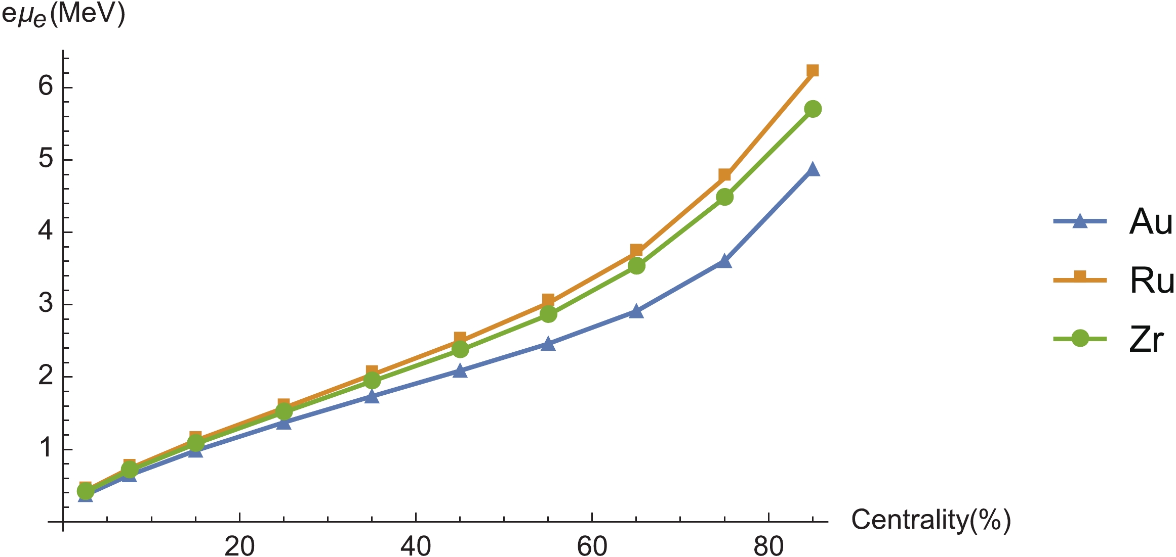
Figure 2. (color online) Centrality dependence of the event-averaged electric chemical potentials induced by the chiral magnetic effect, with triangles for Au, squares for Ru, and circles for Zr.
-
To determine the scalings of the magnitude of the electric chemical potential for different heavy ions, we substitute (9) and (13) into (18), and sort it into several blocks as
$ \begin{align} {\mu}_e({\tau}_f) = \frac{3}{{\pi}^2\ T_f^2}\ \frac{L_\perp B_0}{ S_\perp}\ \frac{1}{{\tau}_f}\ \int_{{\tau}_0}^{{\tau}_f} \,{\rm{d}}{\tau}\ \frac{{\tau} }{1+({\tau}/{\tau}_B)^2}\ {\mu}_{A0}\left(\frac{{\tau}}{{\tau}_0}\right)^{-\frac13} \sqrt{{\rm e}^{3\left( {1-\left( {\frac{{\tau}}{{\tau}_0}} \right)^{2/3}} \right)\left( {\frac{{\tau}_0}{{\tau}_{{\rm{CS}}0}}} \right)}+\frac{3T_0^3}{{\tau}_0\ {\Delta}{\eta}\ S_\perp\ n_{A0}^2}\left[1-{\rm e}^{3\left( {1-\left( {\frac{{\tau}}{{\tau}_0}} \right)^{2/3}} \right)\left( {\frac{{\tau}_0}{{\tau}_{{\rm{CS}}0}}} \right)}\right]}. \end{align} $

(21) The first block,
$ \dfrac{3}{{\pi}^2\ T_f^2} $ , holds identically for the three types of nucleus. The second block,$ \dfrac{L_\perp B_0}{ S_\perp} $ , is determined entirely from the geometry of the nuclei, that is, the distribution of nucleons. The third block,$ \dfrac{1}{{\tau}_f}\ \int_{{\tau}_0}^{{\tau}_f} $ , accounting for the integral average, scales as$ \dfrac{{\tau}_f-{\tau}_0}{{\tau}_f}\sim 1 $ . The fourth block,$ {\mu}_{A0}\left(\dfrac{{\tau}}{{\tau}_0}\right)^{-\frac13} $ , is determined by the initial condition from the glasma, which we already discussed in Section 2. The square root factor accounts for the damping and fluctuation in our stochastic model.We first determine the scaling of the geometrical term
$ \dfrac{L_\perp B_0}{ S_\perp} $ . Throughout the following analysis, the empirical proportionality relationship$ R_0\sim A^{1/3} $ is implied. For$ L_\perp $ and$ S_\perp $ , the geometrical property from the Glauber model is straightforward,$ S_\perp\sim R_0^2 \sim A^{2/3}, \qquad L_\perp\sim R_0\sim A^{1/3}, $

(22) which is also in agreement with (14), if we assume that the number of participants scales with the volume
$ N_{\rm{part}}\sim R^3 \sim A $ .To analyze the magnetic field, we have to know its dependence on the centrality. Note that (19) is the dependence on the impact parameter, but at a given centrality, the averaged impact parameter is different for each type of nuclei. Since we are comparing the signal in each fixed centralities, we have to know how the averaged impact parameter scales for different nuclei in each centrality.
Following from [33], the distribution of the total cross section
$ {\sigma}_{\rm{tot}} $ holds well for$ b<2R_0 $ ,$ \frac{ \,{\rm{d}} {\sigma}_{\rm{tot}}}{ \,{\rm{d}} b}\simeq 2\pi b, $

(23) thus, the total cross section scales is given as,
$ {\sigma}_{\rm{tot}}\sim \int^{R_0} b \,{\rm{d}} b\sim R_0^2\sim A^{2/3}, $

(24) which is a reasonable scaling in term of dimensions. From [47], the following geometric relation between centrality c and impact parameter b also holds to a very high precision for
$ b<2R_0 $ ,$ b(c)\simeq\sqrt{\frac{c\cdot {\sigma}_{\rm{tot}}}{\pi}}. $

(25) Thus, for a given centrality c, the average impact parameter for different nucleus scales with
$ b(c)\sim {\sigma}_{\rm{tot}}^{1/2} \sim A^{1/3}. $

(26) To proceed to determine the scaling of the magnetic field, we take the multiple-pole expansion of (19) and treat the monopole as our scaling of the magnetic field for different nucleus at a given centrality c, thus it is given by
$ B_0(c) \sim Z/b(c)^2 \sim ZA^{-2/3}. $

(27) Therefore, the geometrical combination block scales is given as
$ \frac{L_\perp B_0}{S_\perp}\sim \frac Z A. $

(28) Next, we look at the chemical potential block, without damping and fluctuation effects. The scaling of the initial chemical potential is already discussed in Section 2, and is
$ {\mu}_{A0}\sim A^{1/6} $ , but considering the volume expansion, which contains$ {\tau}_0 $ , it scales as$ {\mu}_{A0}\left(\frac{{\tau}}{{\tau}_0}\right)^{-\frac13}\sim A^{1/9}. $

(29) Lastly, the most ambiguous block is the square root factor accounting for the damping and fluctuation effect. From the above analysis, the scaling of the fluctuation is set by
$ \frac{3T_0^3}{{\tau}_0\ {\Delta}{\eta}\ S_\perp\ n_{A0}^2} \sim A^{-1}. $

(30) However, fluctuation is generally small compared to initial contribution from the glasma. If we neglect it, the square root factor simply scales with
$ 1 $ . Incorporating the contributions from both of them, we may write the scaling of the square root factor as$ A^{-\zeta} $ , with$ 0<\zeta<\dfrac12 $ .Combining all of the above terms together, we have the scaling of the electric chemical potential as
$ {\mu}_e({\tau}_f) \sim \left( {\frac Z A} \right) A^{\frac19} A^{-\zeta} = Z A^{-(\zeta+\frac89)}, $

(31) with
$ 0<\zeta<\dfrac{1}{2} $ . When we consider only the CME from the initial condition,$ \zeta = 0 $ ; when we consider only the fluctuation effect$ \zeta = \dfrac{1}{2} $ . Otherwise,$ \zeta $ lies between them. Our numerical data for Au and isobars suggest a rough value of$ \zeta\simeq\dfrac{1}{4} $ . However, there are deviations in each centrality, mainly due to our simplified scaling of the magnetic field using the monopole. -
To proceed, we will first employ the Cooper-Frye freeze-out procedure [48] to obtain the spectrum of the single particle distribution,
$ E\frac{ \,{\rm{d}} N}{ \,{\rm{d}}^3 p} = \frac{g}{(2\pi)^3}\int p^\mu \,{\rm{d}}^3\sigma_\mu f(x,p), $

(32) where g is the degeneracy factor, taken to be
$ 1 $ for each species of mesons ($ K^\pm $ ,$ \pi^\pm $ ) produced in QGP. The 4-momentum of the particle and Bjorken spacetime 4-velocity are given by$ p^{\mu} = (m_\perp \cosh y,\ p_\perp, m_\perp \sinh y), \quad u^{\mu} = (\cosh {\eta}, 0,0,\sinh{\eta}), $

(33) with
$ m_\perp = \sqrt{p_\perp^2+m^2} $ . Note that y is the particle rapidity and$ {\eta} $ is the spacetime rapidity. Thus, we could expand the Cooper-Frye formula to$ \frac{ \,{\rm{d}} N}{ \,{\rm{d}} \phi \,{\rm{d}} y p_\perp \,{\rm{d}} p_\perp} = \frac{g}{(2\pi)^3}\int \tau_f \,{\rm{d}}{\eta} \,{\rm{d}}^2x\ m_\perp \cosh(\eta-y)f(x,p). $

(34) The phase-space distribution of the i-th particle species at freeze-out time is given in Boltzmann approximation as,
$ f_i(x,p) = {\rm e}^{(p_{\mu} u^{\mu} \pm e{\mu}_e({\tau}_f)+{\mu}_i)/T_f}, $

(35) where
$ \pm{\mu}_e({\tau}_f) $ is the positive or negative electric chemical potential at freeze-out time caused by CME, as in Fig. 2, which is much smaller than the freeze-out temperature$ T_f\simeq {154\; {\rm{MeV}}} $ [49], and$ \mu_i $ is the chemical potential for the i-th species. Here, we consider only pions and kaons in our calculations with respect to heavy ion collisions, with$ {\mu}_{\pi}\simeq {80\; {\rm{MeV}}} $ for pions and$ {\mu}_K\simeq {180\; {\rm{MeV}}} $ for kaons. Thus, we can approximate the distribution to the lowest order in$ {\mu}_e $ as$ {\delta} f_i(x,p) = f_i(\mu_e = 0)\ \frac{\pm e\mu_e({\tau}_f)}{T_f}, $

(36) which leads to the azimuthal distribution of the ith positive or negative charged particle
$ N_\pm^i $ created from CME being$ \begin{split} {\delta} \frac{ \,{\rm{d}} N_\pm^i}{ \,{\rm{d}} \phi} =& \frac{g_i\ S_\perp}{(2\pi)^3}\int\! \,{\rm{d}} m_\perp m_\perp^2 \int\! {\tau}_f \,{\rm{d}} y \,{\rm{d}} {\eta}\ \cosh({\eta}-y)\\&\times f_i(\mu_e = 0)\ \frac{\pm e\mu_e({\tau}_f)}{T_f}. \end{split} $

(37) Here, we used the fact that
$ p_\perp \,{\rm{d}} p_\perp = m_\perp \,{\rm{d}} m_\perp $ . The lower bound of$ m_\perp $ integration is the rest mass of the corresponding meson. The integration domain for particle rapidity should be taken according to the experiments as$ |y|<1 $ , and the spacetime rapidity as$ |{\eta}|<2 $ . Note the sign difference on the right hand side of the above equation; the charge asymmetry of the particle distribution is due to CME. Since the magnetic field points to the upper half of the QGP region from the lower half across the reaction plane, positive charge accumulates in the upper region and negative charge in the lower one. Therefore,$ {\mu}_e $ changes sign across the reaction plane. Similarly, the multiplicity of charged particles from the background is obtained consistently from (34) as$ \frac{ \,{\rm{d}} N_\pm^i}{ \,{\rm{d}} \phi} = \frac{g_i\ S_\perp}{(2\pi)^3}\int\! \,{\rm{d}} m_\perp m_\perp^2 \int\! {\tau}_f \,{\rm{d}} y \,{\rm{d}}{\eta} \cosh({\eta}-y) f_i({\mu}_e = 0),$

(38) where there is no sign difference between positive and negative charges, indicating that the background is electrically neutral.
To acquire the total charged particle multiplicity from CME
$ {\Delta}_\pm $ and from the neutral background$ N_\pm^{bg} $ , index i should be summed over different species. Thus, we define$ {\Delta}_\pm\equiv \sum\limits_i {\delta} N_\pm^i, \qquad N^{bg}_\pm\equiv \sum\limits_i N^i_\pm, $

(39) where again
$ \pm $ denotes positive or negative charge. Note that since we assume the whole QGP to be electrically neutral, the fluctuation of the electric chemical potential is averaged to be zero,$ \langle {\mu}_e({\tau}_f)\rangle = 0 $ , but the two-point correlation is taken to be the square of the electric chemical potential itself,$ \langle {\mu}_e({\tau}_f)^2\rangle\simeq {\mu}_e({\tau}_f)^2 $ . Further, note that our electric chemical potential$ {\mu}_e $ calculated in Section 2 is an effective quantity; it is not$ {\eta} $ -dependent and decouples in the integrals. Then, from (37), (38) and (39), denoting$ {\alpha},{\beta} = \pm $ and$ {\sigma}_\pm = \pm 1 $ , we have the following average and proportionality relations:$ \langle {\Delta}_{\alpha}\rangle = 0, \qquad \frac{\langle {\Delta}_{\alpha}{\Delta}_{\beta}\rangle}{\left\langle { N^{bg}_{\alpha}} \right\rangle \left\langle { N^{bg}_{\beta}} \right\rangle }\simeq{\sigma}_{\alpha}{\sigma}_{\beta}\frac{(e{\mu}_e({\tau}_f))^2}{T_f^2}. $

(40) The average relation on the left is interpreted straightforwardly as the conservation of electric charge. The proportionality relation on the right is a measurement of the asymmetry. The CME induced term
$ {\Delta}_\pm $ is treated as a perturbation to the electrically neutral background as heat bath with temperature$ T_f $ .Subsequently, we analyze the background angular distribution
$ {\rm d}\langle N_\pm\rangle /{\rm d}\phi $ , which reflects the charge-independent evolution of the medium determined by the event-by-event fluctuating initial state. Pursuant to this, we take the Fourier expansion of the background angular distribution as$ \frac{ \,{\rm{d}} \langle N^{bg}_\pm\rangle }{ \,{\rm{d}}\phi} = \frac{\langle N^{bg}_\pm\rangle}{2\pi} \left[1+2\sum\limits_{n = 1} v_n \cos n(\phi-\Psi_{n})\right] , $

(41) where
$ \Psi_n $ indicates the participant plane angle of order n. Note that we have dropped the sine term in the Fourier decomposition because the distribution is symmetric about the participant plane. Coefficient$ v_n $ is defined as the nth order harmonic flow. Typically, the directed flow$ v_1 $ is generally chosen to be$ 0 $ if the distribution is measured in a symmetric rapidity region [13, 50]. Therefore, in the following calculation, we only retained the next leading term from the elliptic flow$ v_2 $ .Next, we assume the following ansatz [1] for the total generated charged single-particle spectrum originating from both the background and the CME:
$ \frac{ \,{\rm{d}} N_\pm}{ \,{\rm{d}}\phi} = \frac{ \,{\rm{d}} \langle N^{bg}_\pm\rangle }{ \,{\rm{d}}\phi}+ \frac1 4 {\Delta}_\pm \sin(\phi-\Psi_{RP}), $

(42) where the form of the CME-induced term is proportional to
$ \sin(\phi-\Psi_{RP}) $ owing to the symmetry of the distribution about the magnetic field, which is perpendicular to the reaction plane, and where the factor$ 1/4 $ is consistent with our definition (39).In contrast to our previous work [30], we choose our correlated two-particle spectrum not only as a product of the single spectrum, but also to include an underlying correlation term proposed in [13] as
$ \rho(\phi_1,\phi_2) = \left\langle\frac{ \,{\rm{d}} N^\alpha}{ \,{\rm{d}} \phi_1^\alpha}\frac{ \,{\rm{d}} N^\beta}{ \,{\rm{d}} \phi_2^\beta}\right\rangle\bigg[1+\sum\limits_{n = 0}^{\infty} a_n \cos n(\phi_1-\phi_2)\bigg], $

(43) with
$ {\alpha},\,{\beta} = \pm $ . The cosine correlation term is reaction-plane-insensitive. Here, we only consider the leading term$ a_1 $ (with normalization leading to$ a_0 = 0 $ ).By employing all these values, two types of two particle correlations,
$ \gamma $ and$ \delta $ , which are measured in the heavy-ion collision experiments, are given as$ \left\{\begin{split} \gamma_{\alpha\beta}& = \left\langle {\cos(\phi_1^\alpha+\phi_2^\beta-2\Psi_{{RP}})} \right\rangle \\ \delta_{\alpha\beta}& = \left\langle {\cos(\phi_1^\alpha-\phi_2^\beta)} \right\rangle , \end{split}\right. $

(44) where the average
$ \left\langle {\cos\varphi} \right\rangle $ of the angle$\varphi = (\phi_1^\alpha+ $ $\phi_2^\beta-2\Psi_{{RP}})$ or$ (\phi_1^\alpha-\phi_2^\beta) $ is taken over events, that is, integrated over$ \phi_1 $ and$ \phi_2 $ as$ \left\langle {\cos\varphi} \right\rangle = \frac{\int\rho(\phi_1,\phi_2)\ \cos \varphi\ \,{\rm{d}}\phi_1^\alpha \,{\rm{d}}\phi_2^\beta}{\int\rho(\phi_1,\phi_2)\ \,{\rm{d}}\phi_1^\alpha \,{\rm{d}}\phi_2^\beta}. $

(45) This will result in
$ \left\{\begin{split} \gamma_{\alpha\beta}& = \langle v_2 a_1 \cos2(\Psi_2-\Psi_{RP})\rangle-\frac{\pi^2}{16}\frac{\langle \Delta_\alpha \Delta_\beta\rangle }{\langle N^{bg}_\alpha\rangle \langle N^{bg}_\beta\rangle}\\ \delta_{\alpha\beta}& = \langle \frac{a_1}{2}(1+v_2^2)\rangle+\frac{{\pi}^2}{16}\frac{\langle \Delta_\alpha \Delta_\beta\rangle }{\langle N^{bg}_\alpha\rangle \langle N^{bg}_\beta\rangle}. \end{split}\right. $

(46) These forms of
$ \gamma $ and$ {\delta} $ correlators are consistent with the proposal discussed in [5, 13]:$ \left\{\begin{split} \gamma_{{\alpha}{\beta}}& = \kappa v_2F_{{\alpha}{\beta}}-H_{{\alpha}{\beta}},\\ \delta_{{\alpha}{\beta}}& = F_{{\alpha}{\beta}}+H_{{\alpha}{\beta}}, \end{split}\right. $

(47) with
$ F_{{\alpha}{\beta}} $ denoting the background and$ H_{{\alpha}{\beta}} $ denoting the CME contribution, and$ \kappa $ being an undetermined factor ranging from$ 1 $ to$ 2 $ . Therefore, by matching the above sets of equations and using (40), we claim that the CME signal takes the following form:$ H_{{\alpha}{\beta}} = \frac{{\pi}^2}{16}\frac{\langle \Delta_\alpha \Delta_\beta\rangle }{\langle N^{bg}_\alpha\rangle \langle N^{bg}_\beta\rangle}\simeq{\sigma}_{\alpha}{\sigma}_{\beta}\ \frac{{\pi}^2}{16}\frac{(e{\mu}_e({\tau}_f))^2}{T_f^2}. $

(48) The difference between the same charge correlation
$ H_{SS} $ and opposite charge correlation$ H_{OS} $ is thus expressed as$ (H_{SS}-H_{OS})\simeq2\cdot\frac{{\pi}^2}{16}\frac{(e{\mu}_e({\tau}_f))^2}{T_f^2}. $

(49) The centrality dependence of
$ 10^4\left(H_{SS}-H_{OS}\right) $ for Au and isobars is shown in Fig. 3. We also plot the signal for AuAu collision at$ {200\; {\rm{GeV}}} $ with data extracted from STAR, by solving (47) as
Figure 3. (color online) Centrality dependence of the CME signal from our stochastic model for AuAu and isobaric collision at
$ \sqrt{s_{{NN}}}={200\; {\rm{GeV}}} $ , with triangles for Au, squares for Ru, and circles for Zr. We also list the data for AuAu collisions at$ \sqrt{s_{{NN}}}={200\; {\rm{GeV}}} $ , extracted from STAR [51, 52], with pentacles, for comparison.$ H_{{\alpha}\beta} = \frac{\kappa v_2 \delta_{{\alpha}\beta}-\gamma_{{\alpha}\beta}}{1+\kappa v_2}, $

(50) where
$ \kappa $ is taken to be$ 1 $ , numerical values of$ \gamma $ and$ \delta $ are taken from [51], and values of$ v_2 $ are taken from [52]. Notably, by adjusting the$ \tau_B $ parameter, the CME signal from our model is in a good agreement with that from the experiments. Moreover, with the same$ \tau_B(\simeq {1.65\; {\rm{fm}}}) $ , we predict the signals for Ru and Zr, which are larger than that of Au, due to the square of the scaling of$ \mu_e({\tau}_f) $ as$ Z^2 A^{-2(\zeta+\frac89)} $ , with roughly$ \zeta\simeq\dfrac{1}{4} $ , as we discussed in Section 3.2. -
We have calculated the axial charge evolution using the stochastic hydrodynamics model, and used it to derive the chiral magnetic effect in off-central collisions of AuAu, RuRu, and ZrZr. By matching the results from our model with the background subtracted experimental data, we have fixed the relaxation time for the magnetic field. We use the same relaxation time to make predictions for the CME signal for collisions of RuRu and ZrZr. Two significant results have been obtained in our analysis.
First, while the axial and vector charges are coupled through the chiral magnetic effect and chiral separation effect, we found that the influence of vector charge on axial charge is negligible at top RHIC collision energy. This allows us to decouple the evolution of axial charge from the vector charge.
Secondly, we study the centrality and system size dependencies of the CME signal. The initial chiral imbalance
$ {\mu}_{A0} $ is found to have only weak centrality dependence. The centrality dependence of the CME signal mainly results from the magnetic field and QGP volume factor. As for the system size dependence, although larger systems provide enhanced magnetic field and chiral imbalance, the electric charge asymmetry characterized by$ e{\mu}_e $ is suppressed due to the larger volume factor. Consequently, we found larger absolute charged particle correlation in isobar collisions than in AuAu collisions.The present study readily generalizes to collisions of large nuclei at higher energies, where we expect that Bjorken flow approximation will still apply. It would be interesting to see if the energy dependence matches with current experimental data at different energies. At lower energies, the Bjorken flow approximation becomes inaccurate. One possible approach to address this issue is to implement stochastic noise numerically in the existing AVFD model. We will report studies along these lines in the future.
We are grateful to Huanzhong Huang, Guoliang Ma, Dirk Rischke, and Gang Wang for discussions. G.R.L also acknowledges the Institute for Theoretical Physics at Frankfurt University for the warm hospitality where part of this work has been done.
Chiral magnetic effect in isobar collisions from stochastic hydrodynamics
- Received Date: 2020-04-09
- Available Online: 2020-09-01
Abstract: We studied the chiral magnetic effect in AuAu, RuRu, and ZrZr collisions at


 DownLoad: