


 Abstract
 HTML
HTML Reference
 Related
 PDF
PDF


-
The inflationary scenario is famed as one of the optimal proposals of describing the evolution of the universe in the very early era. The first inflation proposal was introduced by A. Starobinsky, which was based on a conformal anomaly in quantum gravity [1]. The main goal of the model was to solve the issue of the initial singularity, and it was built based on the assumption of a quasi-de Sitter stage in the very early Universe [2-5]. This model described a graceful exit from the inflationary stage, and in this regard, it can be considered as the first model of inflation. The model played an important role in development of the inflation scenario [2-5]. One year later, an inflationary model was introduced by A. Guth, which aimed to solve the problems of the hot big-bang theory [6]. This scenario, known as old inflation, suffered from the bubble nucleation problem. However, the idea was simple and elegant, and it had a deep impact on the subsequent cosmological inflationary models. The new inflationary scenario [7, 8] suitably solved the problem of Guth's model, wherein the scalar field stands at the top of the effective potential and subsequently slowly rolls down to the bottom. In contrast to the old inflation, which occurs in false vacuum with
$\dot{\phi} = 0$ , here, the stage of inflation occurs by slowly rolling the inflaton toward the minimum of its potential, i.e.,$\dot{\phi} \neq 0$ [2-5]. The main problem of the new inflation is that the density perturbations generated during inflation are very large and consequently unacceptable. This problem is avoided by using a small coupling constant of the scalar field. However, for a small coupling constant, the scalar field is no longer in the state of thermal equilibrium with other matter fields [2-5]. Complete modification of the big-bang theory was presented by the invention of the scenario of Chaotic inflation [9], which could solve the problems of both old and new inflations. An interesting feature of this scenario is that inflation could happen even for a simple potential like$V \propto \phi^n$ .Consequently, numerous inflationary scenarios have been proposed, including non-canonical inflation [10-19], tachyon inflation [20-23], DBI inflation [24-29], G-inflation [30-33], and brane inflation [34, 35]. All of these scenarios have similar assumptions. The scalar field is the dominant component at the time, and inflation occurs by slowly rolling the scalar field from the top toward the minimum of the potential. Notably. applying the idea of inflation in the Starobinsky model leads to significant achievements, where the final result is consistent with the observational data. The model is known as the
$R^2$ Starobinsky-inflation [1]. The process of particle creation and the heating up of the universe occur at the end of inflation during preheating and reheating stages, where the scalar field oscillates around the minimum of its potential with time scales shorter than the Hubble time, and its energy is drained to other matter fields, for instance, radiation [36].In 1995, a new concept of inflation was introduced by A. Berera, known as warm inflation [37]. According to warm inflation, the scalar field remains the dominant component of the universe, however, the interaction between the scalar field and other fields is not ignored. Owing to this interaction, the energy is transferred from the scalar field to the radiation. Therefore, a particle production mechanism occurs during inflation, and the temperature of the Universe does not suddenly drop. The Universe remains warm and full of other particles, a scenario in which reheating is no longer required, and the Universe smoothly enters the radiation era [37-47]. Another difference is with regard to the type of cosmological perturbations. In warm inflation, there are both quantum and thermal fluctuations, and thermal fluctuations dominate. The thermal fluctuations are proportional to the fluid temperature T, and quantum fluctuations are proportional to the Hubble parameter H. Subsequently, the condition of domination of thermal fluctuation leads to the
$T>H$ inequality condition.Numerous studies have investigated different aspects of the warm inflationary scenario for different models [37-39, 42-45]. In the present study, we reconsider the warm inflation, where the tachyon field plays the role of the inflaton. The main motivations for the present work are stated in the following lines. The first reason is the recently proposed swampland conjecture. The recent studies on the effective field theory (EFT) and string theory lead to two swampland criteria [48, 49]: I) imposing an upper bound on the field range, i.e.,
$\Delta\phi < \Delta$ (where$\Delta$ is of the order of unity), which rises from the consideration that the effective Lagrangian in the EFT is valid only for a finite radius; II) placing an upper bound on the gradient of the potential of the field of any EFT, i.e.,$|V'|/V \geq c$ (where the most recent studies determine that c can be even of the order of${\cal{O}}(0.1$ ) [50]). The second criterion implies that the first slow-roll parameter, i.e.,$\epsilon_{\phi} = (V' / V)^2,$ and the tensor-to-scalar ratio,$r = 16\epsilon_{\phi} > 8c^2,$ must not be small. The requirement of satisfying these two criteria could rule out some of the inflationary models; however, a possibility remains for some other models to survive [50-58]. The k-essence model [59-61] is one of them, where$r = 16 c_s \epsilon_{\phi}$ , and the sound speed$c_s$ can be smaller than unity [60]. The tachyon model, which was inspired by the string theory, is known as a subclass of k-essence model, and could be a suitable choice for considering the swampland criteria. The other inflationary model which is able to survive the aforementioned criteria is warm inflationary scenario where the first slow-roll parameter is obtained as$\epsilon = \epsilon_{\phi}/Q$ and tensor-to-scalar ratio is found as$r = (H / T) \; (16 \epsilon_{\phi} / (1+Q)^{5/2})$ [62-71]. The parameter Q is known as the dissipative parameter which in strong dissipative regime is bigger than unity,$Q \gg 1$ . This feature aids the scenario to successfully pass the criteria and satisfy them [51-53, 72-77]. The second motivation is related to the importance of the tachyon field. After the introduction of the tachyon model in cosmological studies [78-81], the model received immense attention and found a place in all areas of cosmology, including the inflation [20-23, 82, 83].The warm inflation, including the tachyon field as the inflaton, has been studied in [84-93]; however, we will reconsider the scenario with a different interaction terms while working with the Hubble parameter instead of the potential, namely the Hamilton–Jacobi formalism [82, 94-99]. The study of the inflationary models is usually performed using three methods:
1. Introducing the potential, which is the most commonly applied method in inflationary studies.
2. Introducing the Hubble parameter, where, instead of the potential, the Hubble parameter is introduced as a function of the scalar field. The method is known as the Hamilton-Jacobi formalism.
3. Introducing the scale factor as a function of time, e.g., the intermediate inflation.
The first approach imposes some restrictions on the form of the potential and evolution of the scalar field. However, in the second approach, several conditions are imposed on the evolution of the Hubble parameter. In general, the Hamilton-Jacobi formalism provides a clear geometrical interpretation and more convenient analysis. Some features of the formalism could be addressed as: 1) More accurate expressions for the slow-roll parameters, 2) neglecting extra assumptions, 3) easy to work with (detailed explanation about the formalism and its features could be found in [95] and references therein).
The main focus of the present work is considering the consistency of the model with observational data and qualitatively considering its agreement with the swampland criteria as well. According to [100], the interaction term in the conservation equations is assumed to include a dissipation coefficient and a sum of energy density and pressure of the scalar field. In this regard, the interaction is different than those the other performed studies on the topic; the interaction term is
$H^2 \Gamma \dot\phi^2$ instead of the usual term$\Gamma \dot\phi^2$ . Another consequence of the selected interaction term is that we have the same definition for the dissipative parameter$Q = \Gamma/3H$ , independent of the type of the scalar field.The dissipation coefficient can be considered as a function of either the scalar field or the temperature, and in some cases, this depends on both the scalar field and the temperature. Here, two different choices are selected for this coefficient. At first, only dependency on the tachyon field is assumed, and in the second case, the coefficient is considered as a function of both the tachyon field and fluid temperature. The main perturbation parameters are obtained for the model, and in comparison with the latest observational data, we attempt to determine the free parameters of the model. In the following step, the self-consistency of the model is considered. The model is constructed based on several assumptions, and we examine their validity for the obtained values of the constants of the model. The self-consistency of the model is an important point that is not sufficiently addressed in studies reported to date.
This paper is organized as follows. In Sec. 2, the dynamical perturbation equations of the model are discussed. Subsequently, in the last part of the section, we rewrite the equations for the strong dissipative regime. To compare the model with observational data, two different choices for the dissipation coefficient are considered in Sec. 3, and they are investigated separately. For each case, the free constants of the model are specified using the observational data, and for each case, we consider the consistency of the results with the main conditions of the model. In Sec. 4, the swampland criteria for the model are discussed. The results of the model are summarized in the conclusion section.
-
The Universe is assumed to be filled with a scalar field driving inflation (referred to as the inflaton) and photon gas. The geometry of the Universe is described by a spatially flat FLRW metric. Then, the Friedmann equation is given as
$3H^2 = \rho_{\phi} + \rho_r,$

(1) where
$M_p^2 = 1/8\pi G = 1$ . As mentioned in the introduction, the inflaton is assumed to be a tachyon fluid, which can be described by a diagonal energy-momentum-tensor,$T_{\phi \nu}^{\mu} = {\rm diag}(-\rho_{\phi},p_{\phi},p_{\phi},p_{\phi})$ ① [81]. The energy density and pressure are given by the following relations, respectively [81]$\rho_{\phi} = \dfrac{V(\phi)}{\sqrt{1-\dot{\phi}^2}}, \; \qquad \; p_{\phi} = -V(\phi)\sqrt{1-\dot{\phi}^2},$

(2) where the dot denotes a derivative with respect to the cosmic time t, and
$V(\phi)$ refers the potential of the tachyon field. Owing to the interaction between the tachyon field and radiation, the energy conservation equations are modified as [100]$\dot{\rho}_{\phi} + 3H(\rho_{\phi}+p_{\phi}) = - \Gamma \; (\rho_{\phi}+p_{\phi}),$

(3) $\dot{\rho}_{r} + 3H(\rho_r+p_r) = \Gamma \; (\rho_{\phi}+p_{\phi}),$

(4) where
$\Gamma$ is the dissipation coefficient, the general form of which can be a function of both the scalar field and temperature. The radiation part has a well-known equation of state as$p_r = \rho_r /3$ . Using Eq. (2) and Friedmann equation (1), the interaction term is obtained as$\Gamma \; (\rho_{\phi}+p_{\phi}) = 3\Gamma H^2 \dot{\phi}^2$

which is different from those interaction terms that have been introduced in [84, 85, 87, 88, 92]. This difference leads to the usual definition of the dissipative parameter as
$Q \equiv \Gamma / 3 H$ .The tachyon field equation of motion is obtained by substituting Eq. (2) into Eq. (3)
${\ddot{\phi} \over 1-\dot{\phi}^2 } + 3 H \dot{\phi} + {V' \over V} = - \Gamma \dot{\phi},$

(5) where prime denotes a derivative with respect to the tachyon field
$\phi$ .To obtain an accelerated expansion phase, it is assumed that the tachyon field dominates the photon gas energy density. Thus, the Friedmann Equation (1) is rewritten as
$H^2 = \rho_{\phi} = \;\dfrac{V(\phi)}{\sqrt{1-\dot{\phi}^2}}\;.$

(6) The second Friedmann equation is obtained by taking the time derivative of Eq. (6) and using Eq. (3)
$\dot{H} = \dfrac{-3H^2}{2}\;(1+Q)\;\dot{\phi}^2.$

(7) Assuming that the Hubble parameter is a function of the tachyon field, i.e.
$H: = H(\phi)$ , and because$\dot{H}: = H'\dot{\phi}$ , the time derivative of the field is found as$\dot{\phi} = \dfrac{-2}{3(1+Q)}\;\dfrac{H'}{H^2}\;.$

(8) Another assumption in the scenario of warm inflation is quasi-stable production of the photon gas, i.e.
$\dot{\rho_{\gamma}}\ll 4H\rho_{\gamma} , \Gamma\dot{\phi}^2$ , in which by imposing this condition on Eq. (4), the radiation energy density is obtained as$\rho_{\gamma} = {3 \over 4} \; H \Gamma = \alpha T^4\;,$

(9) where T is the temperature of the thermal bath, and
$\alpha$ is a well-known Stephen–Boltzman constant.The first slow-roll parameter is defined as
$\epsilon \equiv - \dot{H} / H^2$ , which using Eq. (8) becomes$\epsilon(\phi)\equiv -\dfrac{\dot{H}}{H^2} = \dfrac{2}{3(1+Q)}\;\dfrac{H'^2}{H^4}\;.$

(10) The second slow-roll parameter is
$\epsilon_2\equiv-{\dot{\epsilon}}/{H \epsilon}$ , which after some manipulation, arrives at$\epsilon_2 = \left( 2\epsilon(\phi) - 2\eta(\phi) \right) + {Q \over 1+Q}\left(\epsilon(\phi) - \beta(\phi)\right)\;,$

(11) such that the parameter
$\eta$ and$\beta$ are expressed as follows$\eta(\phi)\equiv \dfrac{4}{3(1+Q)}\;\dfrac{H''}{H^3}, \qquad \beta(\phi)\equiv \dfrac{2}{3(1+Q)}\;\dfrac{\Gamma' H'}{\Gamma H^3}.$

Whereas Hubble parameter is given in terms of the tachyon scalar field, one can extract the potential of the model of Friedmann equation (6) viz.,
$V(\phi) = 3M_P^2 H^2(\phi)\sqrt{1-\dfrac{2}{3}\;\dfrac{1}{(1+Q)}\epsilon(\phi)}\;,$

(12) where Eqs. (8) and (10) have been applied to obtain this expression.
The amount of the Universe expansion during the inflationary times is measured by the number of e-folds, N, defined as②
$N = \int\dfrac{H}{\dot{\phi}}{\rm d}\phi = \dfrac{3}{2}\int_{\phi_e}^{\phi}(1+Q)\;\dfrac{H^3}{H'}{\rm d}\phi\;,$

(13) where the subscript "e" in
$\phi_e$ denotes the tachyon field at the end of inflation.Apart from the evolution of the background parameters, we must know about the perturbative behaviours of the parameters at the inflationary period. Cosmological perturbations are the most important predictions of the inflation. These perturbations can generally be divided into three types as scalar, vector, and tensor perturbations. The vector type is typically ignored because it depends on the inverse of the scale factor and will be diluted exponentially during inflation. The primordial seeds of the large scale structure of the Universe are believed to be the scalar perturbations that are generated during inflation. In the warm inflationary scenario, there are both quantum and thermal fluctuations; however, it is assumed that the thermal fluctuations overcome the quantum fluctuations. The power-spectrum of these fluctuations for the tachyon model is given by [84]
${\cal{P}}_s = { {\rm exp}(-2\chi(\phi)) \over \big( V' /V \big)^2 } \; \delta\phi^2\;,$

(14) in which
$\delta \phi$ is the fluctuation in the scalar field, and the parameter$\chi$ is defined as$\begin{split} \chi (\phi ) =& \int {\left[ {\frac{1}{{(3H + \tilde \Gamma /V)}}\;{{\left( {\frac{{\tilde \Gamma }}{V}} \right)}^{\prime} } + \frac{9}{8}\;\frac{{(\tilde \Gamma /V + 2H)}}{{{{(\tilde \Gamma /V + 3H)}^2}}} } \right.} \\ &\times \left( {\tilde \Gamma + 4HV - \frac{{\tilde \Gamma '(V'/V)}}{{12H(3H + \tilde \Gamma /V)}}} \right) \frac{{V'/V}}{V}\;\Bigg]{\rm d}\phi \;. \end{split}$

(15) For our model,
$\tilde{\Gamma}$ is equal to$3 \Gamma H^2$ , as given by Eq. (5). The scalar spectral index, defined as${\cal{P}}_s = {\cal{P}}_s^{\star} \big( k / k_{\star} \big)^{n_s-1}$ , is another observational parameter that measures the scale-dependency of the power-spectrum, where$n_s = 1$ indicates that the power-spectrum is scale-invariant. This parameter is obtained by taking the log-derivative of the power-spectrum as$n_s-1 = {{\rm d}\ln\big( {\cal{P}}_s \big) \over {\rm d}\ln k}.$

(16) Another type of primordial fluctuations are given by the tensor paramters, which are also known as the primordial gravitational waves. Because the fluid has no role in the tensor perturbations equation, the power-spectrum of tensor perturbations is obtained in the same manner as the cold inflationary scenario, i.e.,
${\cal{P}}_t = H^2 / 2\pi^2$ [85, 87, 88, 101, 102]. The tensor perturbations are measured indirectly through the parameter r, which is defined as the ratio of the power-spectrums of the tensor perturbation to the scalar perturbations,$r = {\cal{P}}_t / {\cal{P}}_s$ . In contrast to the scalar perturbations, there are no exact data for this parameter, and there is only an upper bound$r > 0.064$ . -
Depending on the value of the dissipative parameter Q, the study of warm inflation can be divided into two regimes, namely the strong dissipative regime (SDR) and weak dissipative regime (WDR), which respectively correspond to
$Q \gg 1$ and$Q \ll 1$ . For the remainder of the study, the model is considered only for SDR, where the approximation$(1+Q) \simeq Q$ is used in the equations.In warm inflation, thermal fluctuations dominate over quantum fluctuations, and the corresponding fluctuations in the scalar field are given by
$\delta\phi^2\approx {k_F T}/{2\pi^2}$ , where$k_F = \sqrt {\tilde{\Gamma} H/V}$ [84]. Inserting this value into Eq. (14), the amplitude of the scalar perturbations in SDR becomes${\cal{P}}_s = { {\rm exp}(-2\tilde{\chi}(\phi)) \over \big( 2H'/H \big)^2 } \; {T \over 2\pi^2} \; \sqrt{H},$

(17) and the defined parameter
$\chi$ is reduced to$\begin{split} \tilde \chi (\phi ) =& \smallint \left[ {\frac{{\Gamma '}}{\Gamma } + \frac{9}{8}\;\frac{1}{{3HQ}}\left( {3{H^2}Q - \frac{{(3{H^2}\Gamma )'(2H'/H)}}{{36{H^2}Q}}} \right) } \right.\\&\times \left. { \;\frac{{(2H'/H)}}{{3{H^2}}}} \right]{\rm d}\phi \;. \end{split}$

(18) The scalar spectral index
$n_s$ , which is related to the power-spectrum of the scalar perturbation via (16), is obtained in terms of the slow-roll parameters as$n_s - 1 = {13 \over 4} \; \epsilon(\phi) + {3 \over 2} \; \eta(\phi) + {7 \over 4} \; \beta(\phi).$

(19) Notably, the spectral index is obtained up to the first order of slow-roll parameters.
Using Eq. (17) and the tensor power-spectrum, the tensor-to-scalar ratio is obtained as
$r = {16 H'^2 \over T \sqrt{H}} \; {\rm exp}(2\tilde{\chi}(\phi))$

(20) In the following section, two typical examples are considered for the dissipative coefficient
$\Gamma$ . Further, the Hubble parameter is assumed as a power-law function of the scalar field, i.e.,$H(\phi) = H_0 \phi^n$ for the remainder of the work. -
To verify the accuracy and consistency of any inflationary models, it is required to compare theoretical predictions with observations, e.g. [103-105]. In this regard, the dissipative coefficient
$\Gamma$ must be specified, which can be considered as a function of the scalar field, or in more general cases, it could be a function of both the scalar field and fluid temperature. In the following subsections, we consider both cases. -
As the first case, the dissipation coefficient is taken as a power-law function of tachyon field, i.e.
$\Gamma = \Gamma_0 \phi^m$ , where$\Gamma_0$ and m are constants. From Eq. (8), the time derivative of the tachyon field becomes$\dot{\phi} = -\dfrac{2 n}{\Gamma_0}\;\dfrac{1}{\phi^{m+1}}\;.$

(21) The first slow-roll parameter
$\epsilon$ is determined by substituting the introduced dissipation function into Eq. (10). Evidently, inflation ends as the slow-roll parameter$\epsilon$ reaches unity; therefore, the scalar field is read as$\phi_e^{m+n+2} = {2 n^2 \over H_0 \Gamma_0} \; .$

(22) The scalar field at the time of horizon exit is obtained through the number of e-fold (13) as
$\phi_{\ast}^{m+n+2} = \phi_e^{m+n+2} \; \left( 1 + {(m+n+2) \over n} \; N \right)\;,$

(23) where
$\star$ indicates the time of horizon crossing. The slow-roll parameters, at this edge, are obtained as$\epsilon^\ast = \left( 1 + {(m+n+2) \over n} \; N \right)^{-1} \equiv \bar{N}^{-1} \;,$

(24) $\eta^\ast = {(n-1) \over n} \; \epsilon^\ast\; ,$

(25) $\beta^\ast = {m \over n} \; \epsilon^\ast\; .$

(26) Applying these results to Eq. (19), the scalar spectral index at the time of horizon exit is given by
$ n_s - 1 = \left( {13 \over 4} + {3 \over 2} \; {n-1 \over n} + {7 \over 4} \; {m \over n} \right) \; \bar{N}^{-1}\;, $

(27) where the scalar spectral index only depends on the constants n and m. In contrast, by integrating Eq. (18) and substituting the result into Eq. (17), the power-spectrum reads as
${\cal{P}}_s = {1 \over 8\pi^2 n^{3/2}} \; \left( {\Gamma_0 \over 3\alpha H_0} \right)^{1/4} \; {\exp\left[ - \dfrac{3(2n+m)}{ 8 (m+n+2)} \; \epsilon(\phi) \right] \over \phi^{\textstyle{7m+19n-6 \over 4}}}.$

(28) The tensor-to-scalar ratio is easily derived, such that
$r = 4 n^{3/2} \; \left( {3\alpha H_0^9 \over \Gamma_0} \right)^{1/4} \; \phi^{\textstyle{7m+27n-6 \over 4}} \; \exp\left[ {3(2n+m) \over 8 (m+n+2)} \; \epsilon(\phi) \right].$

(29) Subsequently, using Eqs. (23) and (24), the power spectrum and tensor-to-scalar ratio are obtained at the time of horizon crossing.
The first conclusion that can be made from Eqs. (28) and (29) is that the constant n must be positive, otherwise there will be an imaginary value for the parameters
${\cal{P}}_s$ and r, which is unphysical.Hence, to constrain the free parameters of the model, the results at the time of horizon crossing must be examined with data. At this time, the scalar spectral index depends on both parameters n and m. The situation is different for the tensor-to-scalar ratio, where besides n and m, the other two constants
$\Gamma_0$ and$H_0$ also appear in the definition of$r(t = t_{\star})$ . Based on Planck data, an exact value for the amplitude of the scalar perturbations exists, and there are also several statements regarding the energy scale of inflation. Thus, from the energy scale of inflation, Eq. (12), the constant$H_0$ is determined as③$H_0 = \bar{V}^{\star} \; \Gamma_0^{\textstyle{n \over m+2}}, \qquad \bar{V}^{\star} \equiv { \left( V^{\star} / 3 \right)^{\textstyle{m+n+2 \over 2(m+2)}} \over \left( 2n^2 \bar{N} \right)^{\textstyle{n \over m+2}} },$

(30) where
$V^{\star}$ is the energy scale of inflation. Substituting the obtained$H_0$ in the amplitude of the scalar perturbations,$\Gamma_0$ is extracted as$\Gamma_0 = \left( {\cal{P}}_s^{\star} \over D \right)^{\textstyle{4(m+2) \over 8m+18n-4}},$

(31) where the parameter D is defined as
$D = {1 \over 8\pi^2 n^{3/2}} \; {1 \over \big( 3\alpha \bar{V}^{\star} \big)^{1/4}} \; { \exp\left[ - \dfrac{3(2n+m)}{8 (m+n+2) \; \bar{N}} \, \right] \over \big( 2n^2 \bar{N} \big)^{\textstyle{7m+19n-6 \over 4(m+n+2)}}} \;.$

From Eqs. (30) and (31), both perturbation parameters
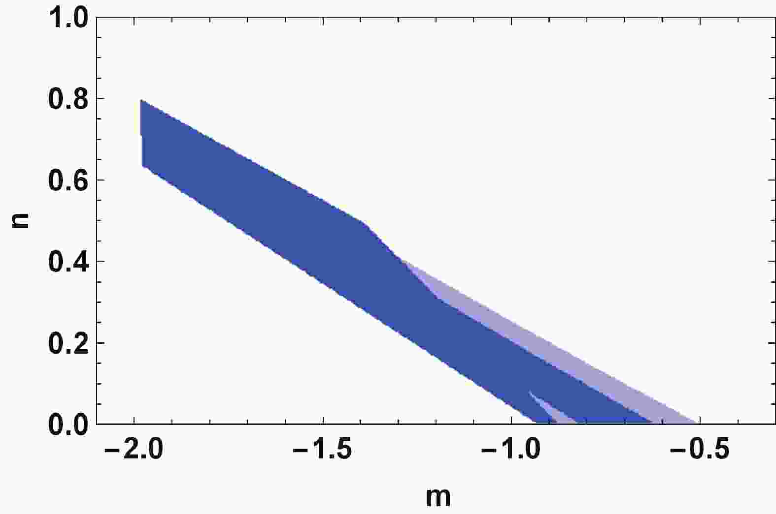
$n_s$ and r depend only on n and m. Utilizing the Planck$r-n_s$ diagram, a set of points is obtained for n and m, where any$(n,m)$ point in the set result of the model is in good consistency with observation. Fig. 1 illustrates this set of points, where the dark blue color determines the$(n,m)$ points for which our model is in agreement with 68% CL of Planck$r-n_s$ diagram, whereas the light blue color is related to 95% CL.
Figure 1. (color online) Parametric plot of
$(n,m)$ .The formulation is not complete. To build the model, we made two main assumptions, and we aim to determine whether the assumptions remain valid for all
$(n,m)$ points in Fig. 1. Subsequently, it is important to verify these assumptions for the whole duration of inflation. In the first postulation, that is in the warm inflationary scenario, the thermal fluctuations must dominate over the quantum fluctuations, described by the condition$T > H$ . The second assumption is that the model is restricted to the SDR, where the dissipative parameter is larger than unity, i.e.,$Q > 1$ . Therefore, we are interested only in the values of$(n,m)$ that satisfactorily pass the conditions and simultaneously put the model in agreement with data. These values are depicted in Fig. 2.
Figure 2. (color online) Parametric plot of
$(n,m)$ , where for each point of this area, the model perfectly meets the observational data, and main assumptions of the model are properly satisfied.Although at the first step, a larger range for the parameters n and m can be found, the range is tightened by imposing the model conditions. The final result shows that only for a small range of the parameter
$(n,m)$ , the model comes to an agreement with the data and simultaneously satisfies the aforementioned conditions.The behavior of
$T/H$ and the dissipative parameter Q are depicted in Figs. 3 and 4 for different values of n and m. With passing time and approaching the end of the inflation, both of these parameters exhibit an increasing trend.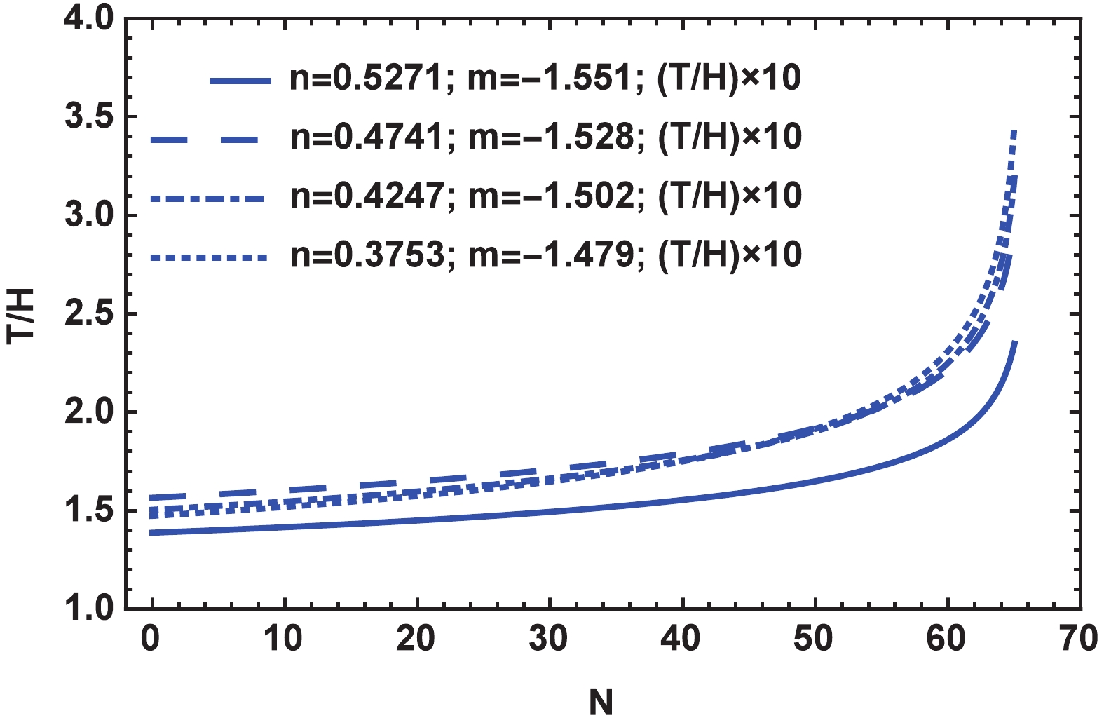
Figure 3. (color online) Behavior of
$T/H$ during inflation for different values of n and m selected from Fig. 2. The plots indicate that both conditions$T/H > 1$ and$Q \gg 1$ are perfectly satisfied.
Figure 4. (color online) Behavior of Q during inflation for different values of n and m selected from Fig. 2. The plots indicate that both conditions
$T/H > 1$ and$Q \gg 1$ are perfectly satisfied.Table 1 lists the numerical results for the main perturbation parameters,
$T/H$ and the dissipative parameter Q for different values of n and m, presented in Fig. 2.n m $\phi_{\star}$ 

$\phi_e$ 

$\Gamma_0$ 

$H_0$ 

$n_s$ 

r $T/H$ 

Q $0.5765$ 

$-1.582$ 

$105.91$ 

$0.9120$ 

$1.06 \times 10^{3}$ 

$6.86 \times 10^{-4}$ 

$0.9765$ 

$1.27 \times 10^{-8}$ 

$14.51$ 

$21.91$ 

$0.5271$ 

$-1.551$ 

$89.43$ 

$0.6551$ 

$9.96\times 10^{2}$ 

$8.42 \times 10^{-4}$ 

$0.9732$ 

$5.43 \times 10^{-9}$ 

$13.87$ 

$34.70$ 

$0.4741$ 

$-1.528$ 

$105.14$ 

$0.6093$ 

$8.14 \times 10^{2}$ 

$8.81 \times 10^{-4}$ 

$0.9689$ 

$1.10 \times 10^{-9}$ 

$15.65$ 

$27.61$ 

$0.4247$ 

$-1.502$ 

$90.33$ 

$0.4193$ 

$7.62 \times 10^{2}$ 

$1.05 \times 10^{-3}$ 

$0.9650$ 

$4.53 \times 10^{-10}$ 

$15.04$ 

$41.05$ 

$0.3753$ 

$-1.479$ 

$81.04$ 

$0.2891$ 

$6.99 \times 10^{2}$ 

$1.22 \times 10^{-3}$ 

$0.9607$ 

$1.70 \times 10^{-10}$ 

$14.73$ 

$54.94$ 

$0.3295$ 

$-1.448$ 

$52.73$ 

$0.1506$ 

$7.46 \times 10^{2}$ 

$1.54 \times 10^{-3}$ 

$0.9572$ 

$1.64 \times 10^{-10}$ 

$12.22$ 

$140.2$ 

$1$ 

$2$ 

$52.07$ 

$16.36$ 

$1.60 \times 10^{-2}$ 

$1.06 \times 10^{-4}$ 

$1.0207$ 

$4.23 \times 10^{7}$ 

$10.00$ 

$2631$ 

$2$ 

$1$ 

$60.90$ 

$21.97$ 

$4.77 \times 10^{-1}$ 

$3.26 \times 10^{-6}$ 

$1.0298$ 

$6.75 \times 10^{13}$ 

$9.15$ 

$799.4$ 

$2$ 

$0$ 

$381.86$ 

$112.87$ 

$4.37 \times 10^{-1}$ 

$1.12 \times 10^{-7}$ 

$1.0305$ 

$9.82 \times 10^{16}$ 

$20.82$ 

$8.88$ 

Table 1. Numerical results of case.
The last three rows of the table represent the choices of n and m in the canonical cases. Fig. 2 shows that these values are out of the range; therefore, the results are not consistent with observational data. Table 1 represents the numerical result, where the scalar spectral index is found to be larger than unity, and the tensor-to-scalar ratio is very large, and confirms our first conclusion.
It is crucial for any inflationary model to verify whether the inflation ends at all. In this regard, the evolution of the slow-roll parameter
$\epsilon$ is considered. Fig. 5 portrays the behavior of$\epsilon$ versus the number of e-fold for different values of n and m. The plot states that$\epsilon$ increases with time and approaches the end of inflation. Eventually, it arrives at one, stating that inflation ends, and the Universe exits from the accelerated expansion phase.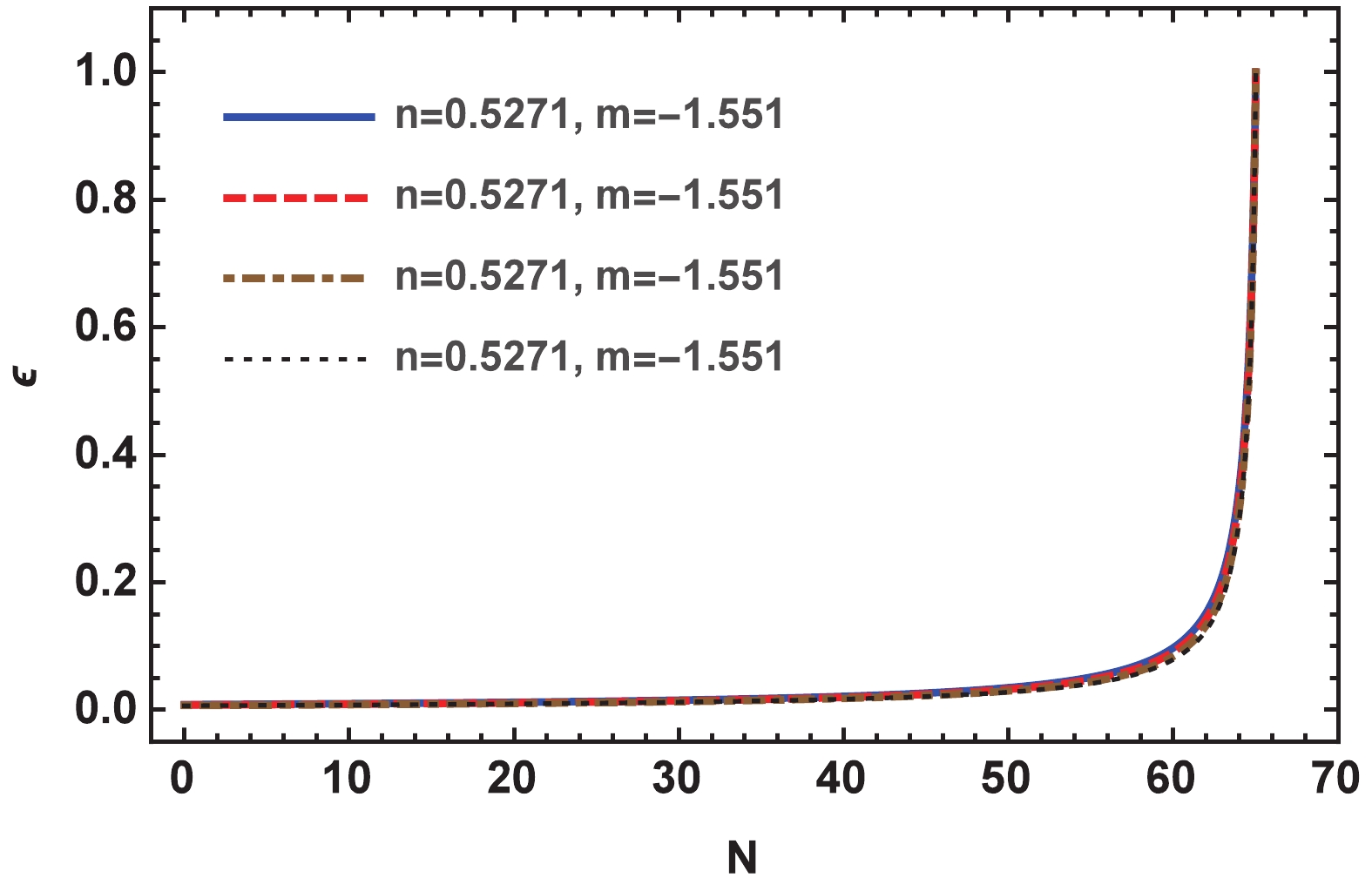
Figure 5. (color online) Behavior of slow-roll parameter
$\epsilon$ versus number of e-fold for different values of n and v selected from Fig. 2. -
In this section, we consider a more general case, where the dissipation coefficient is a function of both the tachyon field and the temperature. A common choice is [101, 106, 107]
$\Gamma = \Gamma_0\dfrac{T^m}{\phi^{m-1}}.$

(32) The temperature of the fluid could be found in terms of the tachyon field from the following relation
$\rho_r = \alpha T^4 = {3 \over 4} \; \Gamma H \; \dot{\phi}^2,$

(33) where the time derivative of the field is obtained from Eq. (8). Using the definition of the dissipation coefficient, the temperature is expressed in terms of the field as
$T^{m+4} = {3 n^2 \over \alpha} \; {H_0 \over \Gamma_0} \; \phi^{m+n-3}.$

(34) Inserting this result in the definition of
$\Gamma$ , Eq. (32), the parameter is read in terms of the scalar field as$\Gamma = \bar{\Gamma}_0 \; \phi^b,$

(35) where
$\bar{\Gamma}_0 \equiv \Gamma_0 \; \left( {3 n^2 \over \alpha} \; {H_0 \over \Gamma_0} \right)^{\textstyle{m \over m+4}}, \qquad b \equiv {nm-6m+4 \over m+4}.$

The scalar field at the end of inflation is derived from the relation
$\epsilon = 1$ , which indicates the end of acceleration expansion phase. Subsequently, following the same process as the previous case, the scalar field at the time of horizon crossing is achieved, such that$\begin{split} \phi _ * ^{b + n + 2} =& \phi _e^{b + n + 2}\;\left( {1 + \frac{{b + n + 2}}{n}\;N} \right) \equiv \phi _e^{b + n + 2}\tilde N,\\ \phi _e^{b + n + 2} =& \frac{{2{n^2}}}{{{{\bar \Gamma }_0}{H_0}}}. \end{split}$

(36) Substituting the above relation in the definition of the slow-roll parameters, one could compute these parameters at the horizon crossing time in terms of the number of e-fold as
$\epsilon^\ast = \tilde{N}^{-1},$

(37) $\eta^\ast = {n-1 \over n} \; \epsilon^\ast,$

(38) $\beta^\ast = {b \over n} \; \epsilon^\ast.$

(39) Inserting the above parameters in Eq. (19), the scalar spectral index is obtained
$n_s - 1 = \left( {13 \over 4} + {3 \over 2} \; {n-1 \over n} + {7 \over 4} \; {b \over n} \right) \; \tilde{N}^{-1},$

(40) which states that the parameter depends on the constants n and m. The power-spectrum of the scalar perturbation and tensor-to-ratio have the same form as obtained in Eqs. (28) and (29), where
$\Gamma_0$ and m are replaced by$\tilde{\Gamma}_0$ and b, respectively.As in the first case, the energy scale of the inflation is utilized to determine the constant
$H_0$ , which arrives to the following expression$H_0 = \tilde{V}^{\star} \; \Gamma_0^{\textstyle{-n \over m-3}}, \qquad \tilde{V}^{\star} \equiv { \left( V^{\star} / 3 \right)^{\textstyle{nm+2n-2m+6 \over -4(m-3)}} \over \left[ 2n^2 \tilde{N} \left( {\displaystyle{\alpha \over 3n^2}} \right)^{\textstyle{m \over m+4}} \right]^{\textstyle{-n(m+4) \over 4(m-3)}} }.$

(41) Applying the above relation in the power-spectrum of the scalar perturbation, and computing the power-spectrum for
$t = t_{\star}$ , the other constant of the model can be specified, such that$\Gamma_0 = \left( {\cal{P}}_s^{\star} \over \tilde{D} \right)^{1/g},$

(42) where the defined constants are expressed as
$ \begin{split} \tilde{D} &\equiv {\left( \dfrac{3n^2}{\alpha} \right)^{\textstyle{m \over 4(m+4)}} \tilde{V}^{\star f} \over 8\pi^2 n^{3/2} (3\alpha)^{1/4}} \; {\exp\left[ \dfrac{-3 (2n+b)} {8(b+n+2) \, \tilde{N}} \right] \over \left( 2n^2 \tilde{N} \left( \dfrac{\alpha}{3n^2} \right)^{\textstyle{m \over m+4}} \right)^{q}}, \\ q &\equiv {7 b +19n-6 \over 4(b+n+2)}, \\ f &\equiv {2q(m+2)-1 \over m+4}, \\ g & \equiv {4q+1 \over m+4} - {n f \over m-3}. \end{split}$

Inserting Eqs. (41) and (42) into the tensor-to-scalar ratio yields
$r^{\star} = { 4 n^{3/2} (3\alpha)^{1/4} \over \left( \dfrac{3n^2}{\alpha} \right)^{\textstyle{m \over 4(m+4)}}} \; {\left( 2n^2 \tilde{N} \left( \dfrac{\alpha}{3n^2} \right)^{\textstyle{m \over m+4}} \right)^{p} \over \exp\left[ \dfrac{-3 (2n+b)}{ 8(b+n+2) \, \tilde{N}} \right]} \; {H_0^{\textstyle{8m-2p(m+2)+36 \over 4(m+4)}} \over \Gamma_0^{\textstyle{4p \over m+4}}},$

(43) in which the parameter p is defined as
$p \equiv {7b+27n-6 \over 4(b+n+2)}.$

From Eqs. (41) and (42), the tensor-to-scalar perturbation (43) depends on the constants n and m. In contrast, the scalar spectral index (40) depends only on these two constants. Using the Planck
$r-n_s$ diagram, the valid values of n and m are elucidated, for which the model prediction about the scalar spectral index and tensor-to-scalar ratio perfectly meet the observational data. These values are plotted in Fig. 6.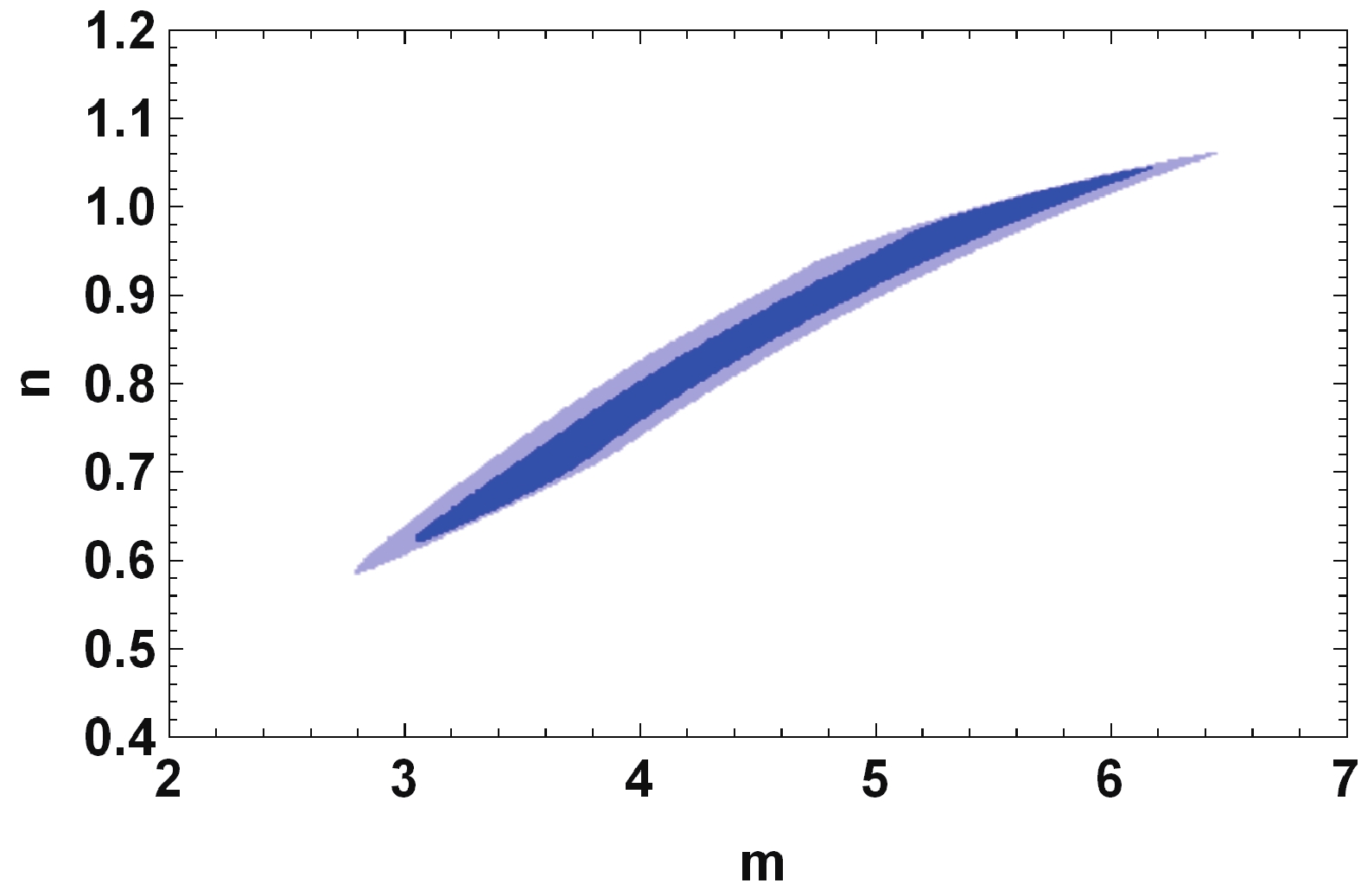
Figure 6. (color online) Parametric plot of
$ (n,m)$ .The following step is to examine whether these values of
$(n,m)$ are consistent with the assumptions, i.e.$T/H>1$ and$Q\gg 1$ , that were used for building the model. The fluid temperature is given in Eq. (34), and the dissipative parameter for the case is read as$Q = {\Gamma_0 \over 3H_0} \; \left( {3n^2 \over \alpha} \; {H_0 \over \Gamma_0} \right)^{\textstyle{m \over m+4}} \; {1 \over \phi^{\textstyle{2(2n+3m-2) \over m+4}}}.$

(44) Inserting
$\phi_{\star}$ and using Eqs. (41) and (42), both temperature and the dissipative parameter are expressed in terms of the constants n and m. Further investigation indicates that the obtained range of$(n,m)$ , that has been plotted in Fig. 6, can perfectly satisfy both conditions. To gain a better insight, Figs. 7 and 8 display the behavior of$T/H$ and Q, respectively,for different choices of n and m. The figures clearly display that $T/H$ increases with passing time and approaches the end of inflation, while the dissipative parameter Q exhibits completely different behavior, in that it initiates from high values and subsequently decreases. However, the most important point is that during the inflation, these parameters are always significantly larger than one, and the conditions$T/H > 1$ and$Q > 1$ are perfectly satisfied.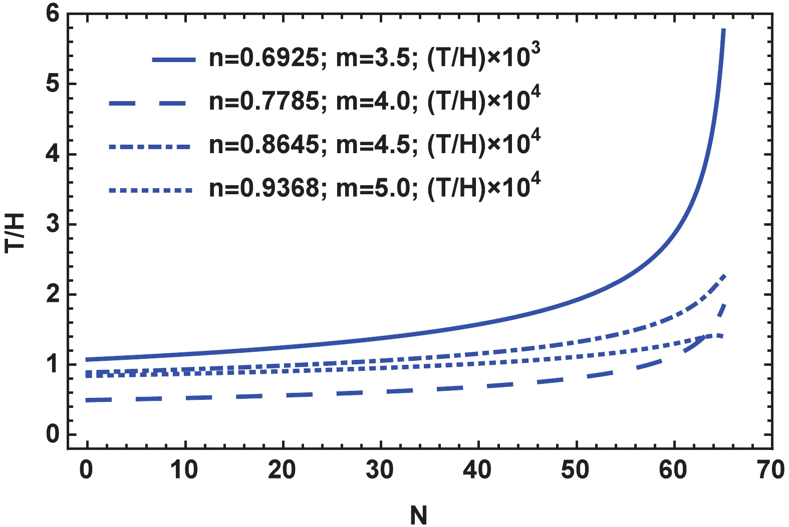
Figure 7. (color online) Behavior of
$ T/H$ during inflation for different values of n and m selected from Fig. 6. The plots indicate that both conditions$ T/H > 1$ and$ Q \gg 1$ are perfectly satisfied.
Figure 8. (color online) Behavior of Q during inflation for different values of n and m selected from Fig. 6. The plots indicate that both conditions
$ T/H > 1$ and$ Q \gg 1$ are perfectly satisfied.To gain a numerical insight on the result, the perturbation parameters of the model, as well as the temperature and dissipative parameters are presented in Table 2, where they are found out for different values of n and m.
n m $\phi_{\star}$ 

$\phi_e$ 

$\Gamma_0$ 

$H_0$ 

$n_s$ 

r $T/H$ 

Q $0.6547$ 

$3.23$ 

$3.74 \times 10^{-6}$ 

$1.72 \times 10^{-8}$ 

$1.06 \times 10^{19}$ 

$3.26 \times 10^{-3}$ 

$0.9703$ 

$0.0161$ 

$319.35$ 

$1.04 \times 10^{23}$ 

$0.7175$ 

$3.66$ 

$5.13 \times 10^{-6}$ 

$1.47 \times 10^{-8}$ 

$2.10 \times 10^{18}$ 

$5.69 \times 10^{-3}$ 

$0.9662$ 

$0.0046$ 

$2019.82$ 

$6.50 \times 10^{23}$ 

$0.7889$ 

$4.02$ 

$2.06 \times 10^{-6}$ 

$5.23 \times 10^{-9}$ 

$2.12 \times 10^{17}$ 

$0.0279$ 

$0.9675$ 

$0.0005$ 

$3782.75$ 

$1.27 \times 10^{24}$ 

$0.8374$ 

$4.35$ 

$1.55 \times 10^{-6}$ 

$3.06 \times 10^{-9}$ 

$3.02 \times 10^{16}$ 

$0.0667$ 

$0.9665$ 

$0.0002$ 

$9406.08$ 

$1.39 \times 10^{24}$ 

$0.9202$ 

$4.89$ 

$4.86 \times 10^{-7}$ 

$7.48 \times 10^{-10}$ 

$2.20\times 10^{14}$ 

$0.5883$ 

$0.9678$ 

$0.0003$ 

$10646.8$ 

$5.99 \times 10^{22}$ 

$0.9630$ 

$5.25$ 

$3.38 \times 10^{-7}$ 

$3.99 \times 10^{-10}$ 

$9.89 \times 10^{12}$ 

$1.5566$ 

$0.9673$ 

$0.0011$ 

$12190$ 

$3.31 \times 10^{21}$ 

$2$ 

$1$ 

$6.55$ 

$1.93$ 

$2.04 \times 10^{11}$ 

$2.12 \times 10^{-8}$ 

$1.0305$ 

$6.00 \times 10^{-27}$ 

$396.85$ 

$7.26 \times 10^{9}$ 

$1$ 

$-1$ 

$3.98$ 

$1.43$ 

$3.71 \times 10^{2}$ 

$2.34 \times 10^{-7}$ 

$1.0217$ 

$8.69 \times 10^{-15}$ 

$658.79$ 

$3.32 \times 10^{14}$ 

Table 2. Numerical results of case.
The typical values of n and m that we encounter in the canonical cases are listed in the last two rows of Table 2. Based on Fig. 6, these points are beyond our range of interest, and the results are expected to be inconsistent with observation. Table 2 lists the numerical results and indicates that although the predicted r agrees with the data, the result for the scalar spectral index is larger than unity and clearly in tension with data. Consequently, these values of n and m are not suitable for the presented model.
To verify the smooth exit of inflation, the evolution of the first slow-roll parameter
$\epsilon$ is investigated and plotted in Fig. 9.$\epsilon$ increases by approaching the end of inflation, and eventually reaches the value of one. Therefore, inflation ends at this time, and the universe exits the inflationary stage.
Figure 9. (color online) Behavior of slow-roll parameter
$ \epsilon$ with respect to number of e-fold for different values of n and m selected from Fig. 6. -
One of the best candidates to describe quantum gravity may be string theory, which provides a landscape containing consistent low-energy EFTs that can formulate a quantum theory. However, all other low-energy EFTs exist a bigger region known as a swampland. The EFTs that live on swampland contradict the string theory. Building a model based on the consistent EFT, which lives on the landscape, requires a mechanism to separate the consistent and inconsistent EFTs. These efforts resulted in several conjectures, where the swampland criteria represent the most recent proposal. The swampland criteria have been introduced in [48], and they were subsequently refined in [49]. In brief, they are listed as follows:
● C1: Distance conjecture: it is an upper bound that confines the scalar field excursion in the field space as
$\Delta \phi \leqslant \delta \sim {\cal{O}}(1).$

(45) ● C2: de Sitter conjecture: it imposes a lower bound on the gradient of the potential, stating that slope of a positive potential,
$V>0$ , of the scalar field should satisfy the following bound${|V_{\phi}| \over V} \geqslant c \sim {\cal{O}}(1),$

(46) and the refined version of this conjecture is given by
${|V_{\phi}| \over V} \geqslant c \sim {\cal{O}}(1), \quad {\rm{or}} \quad {V_{\phi\phi} \over V} \geqslant -c' \sim -{\cal{O}}(1).$

(47) This is given in Planck units, where
$M_p = 1$ . The exact value of the constant c depends on the detail of the compaction, which states that it could be larger than$\sqrt{2}$ . However, further investigation shows that it could be smaller than unity, even of order${\cal{O}}(0.1)$ , and the important criterium is that it must be positive [50].Inflation is believed to occur at the energy level below the Planck energy scales, where it can be described by low-energy EFT [51-53]. Therefore, it is in our interest to build the inflationary model in the framework of a consistent low-energy EFT that stands in the landscape. In this regard, despite having an agreement with the observational data, which have been investigated previously, the inflationary model should also satisfy two swampland criteria. In the previous sections, the warm inflationary scenario was considered in SDR, where the tachyon field had the role of the inflaton. In the previous sections, the constants of the model were determined in comparison with the observational data. Here, we determine whether the obtained results put the model in consistency with the swampland criteria.
In the first case, where the dissipation coefficient is picked out as a power-law function of the scalar field, a narrow range is obtained for the constants n and m, for whose values the model is in agreement with observational data. However, for these values of n and m, the difference of the scalar field at the times of horizon crossing and end of inflation is of order
${\cal{Q}}(10)$ or sometimes even larger, i.e.,${\cal{Q}}(10^2)$ , which is evident from Table 1. Therefore, it is concluded that although the model is in good consistency with observational data, it does not satisfy the first swampland criterion. The result is different for the second case of the dissipation coefficient, where the parameter$\Gamma$ is a function of both the scalar field and the temperature. The determined values of n and m state that the scalar field values at the end of inflation and also at the beginning of the horizon crossing time are smaller than unity, and Table 2 shows this conclusion, which in turn indicates that the field excursion during inflation is smaller than unity. Therefore, the first swampland criterion is satisfied for the second case of the presented model.The second criterion has received more attention in previous studies, as it seems to be in direct tension with one of the fundamental assumptions of the standard inflationary scenario. The standard inflationary scenario is typically explained by means of the slow-roll parameters. The slow-roll parameter
$\epsilon$ is defined as$\epsilon \simeq V'^2 / 2 V^2$ , which must be smaller than unity to achieve an accelerated expansion phase. In contrast, based on the second swampland criterion, it must be larger than a constant c, which is of order of unity; however,$c \approx 0.1$ could also be employed. Assuming the latent value, the slow-roll parameter$\epsilon$ is obtained as$\epsilon = 0.005$ (for the best case), which is sufficiently small to yield a desire accelerated expansion phase. However, this problem is encountered upon examination of the tensor-to-scalar ratio r with data. Based on the standard inflation model, the parameter is given by$r = 16 \epsilon$ , which for the aforementioned value of$\epsilon$ is acquired at approximately$r = 0.08$ , which is in tension with observational data. The problem might be solved for the generalized model of inflation, such as k-essence and multi-field inflation. In the k-essence model of inflation, the tensor-to-scalar ratio is modified as$r = 16 c_s \epsilon$ , where$c_s$ is the sound speed that could be on the order of$0.1$ [50]. Furthermore, warm inflation, particularly when the model is considered in SDR, could suit the swampland criteria. In warm inflation, the first-slow-roll parameter is generalized as$\epsilon = \epsilon_{\phi} / Q$ , where$\epsilon_{\phi}$ is the same slow-roll parameter that we have in cold inflation, i.e.,$\epsilon_{\phi} = V'^2 / 2 V^2$ , and Q is the dissipative parameter, which is significantly larger than unity in SDR. The second swampland criterion implies that$\epsilon_{\phi} = Q \epsilon > c^2/2$ . Here, we employed the tachyon field as the inflaton, where the first slow-roll inflation is given by Eq. (10) in terms of the Hubble parameter. The potential of the field is related to the Hubble parameter through the relation$V(\phi) = 3H^2 \sqrt{1 - 2 \epsilon /3Q}$ . As the first slow-roll parameter$\epsilon$ is small, also due to the fact that we are working in SDR, the last term can be ignored, such that we obtain, to a good approximation,$V(\phi) = 3 H^2$ . Therefore, the gradient of the potential is given by$V' / V = 2 H' / H$ , and by applying Eq. (10), the second criterion is read as${V' \over V} \simeq 2 {H' \over H} = \left( 6 Q H^2 \epsilon \right)^{1/2}.$

(48) According to the second swampland criterion, the gradient of the potential must be larger than the constant c that is on the order of unity. From Table 1, which lists the values of the parameters of the model for the first case of the dissipation parameter, implies that it is unlikely to arrive at consistency between the model and the criterion. To gain a better understanding, Fig. 10 displays the gradient of the potential with respect to the number of e-fold N from the beginning of inflation to the end. It clearly indicates that the potential gradient increases by approaching the end of inflation; however, it never reaches one.
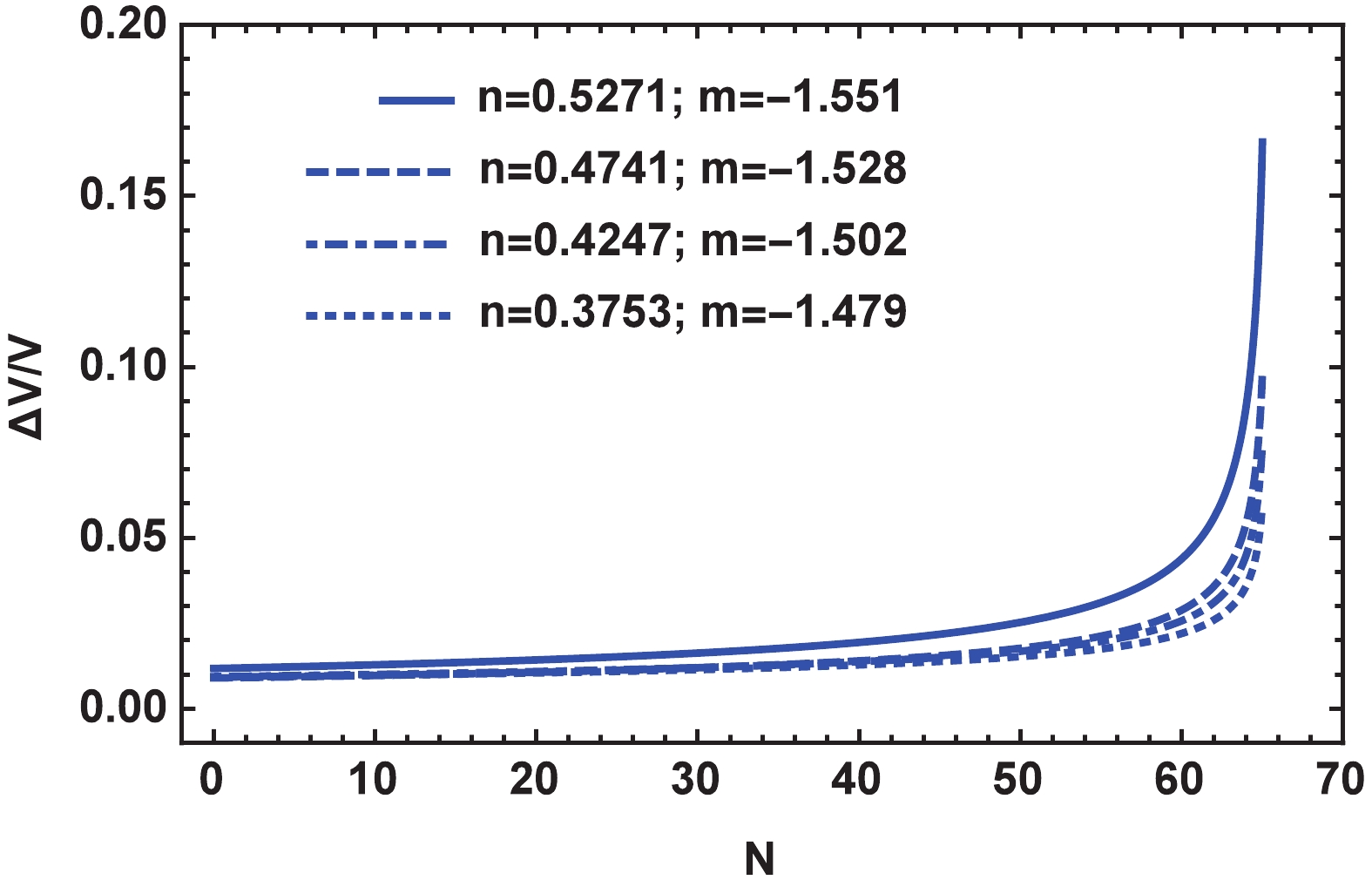
Figure 10. (color online) Behavior of
$ \Delta V/V$ with respect to number of e-fold during the inflation.The situation is different for the second case, which is mostly because of the high value of the dissipative parameter Q for the case. The potential gradient of the field for this case is depicted in Fig. 11, where it is clearly realized that
$\Delta V/V$ is larger than one during the whole inflation duration, and the second swampland criterion is satisfied.
Figure 11. (color online) Behavior of
$ \Delta V/V$ with respect to number of e-fold during inflation.In brief, the first choice of the dissipation coefficient for the tachyon scalar field is in excellent agreement with observational data; however, it satisfies none of the swampland criteria. In contrast, the second choice of the dissipation coefficient yields our desired result; it is in agreement with observational data and simultaneously satisfies the swampland criteria.
-
The scenario of the two-component warm inflation, including the tachyon field as the inflaton and photon gas, was considered. The Universe is assumed to be filled with the scalar field and radiation interacting with each other, and energy is transferred from the scalar field to radiation. The interaction term includes a dissipation coefficient as well as the sum of the energy density and the pressure of the inflaton, which yields the familiar term,
$\Gamma \dot{\phi}^2$ for the case of the standard model of scalar field. This type of interaction is different for each model; however, it approaches the same dissipative parameter,$Q = \Gamma / 3H$ , regardless of the type of the scalar field model.The warm inflation scenario is typically considered in two different regimes, namely the weak and strong dissipative regimes that correspond to
$Q \ll 1$ and$Q \gg 1$ , respectively. This study was restricted to the strong dissipative regime. Employing this assumption, the main dynamical and perturbation parameters were derived for the model. To examine the validity of the model, two different choices of the dissipation coefficient were studied. The dissipation coefficient is a function of the scalar field or temperature, or in some cases, both. In this study, two choices were taken into account for$\Gamma$ . In the first case, it was as a function of the tachyon field, and in the second case, a more general case was considered, i.e., a function of both the tachyon field and temperature.Both cases were investigated in detail, and the free parameters of the model were determined using the observational data. By calculating the slow-roll parameters at the horizon crossing, the scalar spectral index was obtained in terms of the constants n and m. Subsequently, using the energy scale of inflation and the amplitude of the scalar perturbations, the other constants,
$H_0$ and$\Gamma_0$ , were determined. These results indicate that at the horizon crossing, the tensor-to-scalar ratio only depends on n and m. Comparing the theoretical results with the Planck$r-n_s$ diagram, we found a set of$(n,m)$ points, for which the model could perfectly meet the data. However, to obtain ultimately consistent results, the validity of the first assumptions of the model must also be investigated. The thermal fluctuation are assumed to dominate the quantum fluctuations, i.e.,$T/H > 1$ , and it was also supposed that inflation occurs in SDR, i.e.,$Q>1$ . Therefore, in addition to considering the consistency of the model with the data, the self-consistency of the model was also addressed. We attempted to verify whether the obtained set of$(n,m)$ points could guarantee the conditions. Examining these conditions for the first case demonstrated that they are violated for some of the points within the set. Only few points could guarantee the assumptions of the model and simultaneously ensure that the model is in agreement with the data. The situation, however, is better for the second case, where for all obtained$(n,m)$ points, the conditions are fulfilled, and moreover the results about the scalar spectral index and tensor-to-scalar ratio are in good agreement with the data.The final part of the work was devoted to the recently proposed swampland conjectures. Arguably, any inflationary model must be in consistency with these conjenctures, although they are not completely approved to date. There are two conditions that place an upper bound on the distance of the scalar field, and the second condition imposes a lower bound on the gradient of the potential of the scalar field. The criteria could rule out some of the inflationary models; however, there is a strong belief that the warm inflation is capable of satisfying the criteria; mostly because of the presence of the dissipative parameter Q that occurs large in SDR. However, to obtain a precise conclusion, the model must be examined quantitatively. In this regard, both cases of the dissipation coefficient were examined, which determined that the first case could not satisfy even one of the criteria. In contrast, for the second case, where the dissipation coefficient is a function of both the scalar field and the temperature, the model satisfies both swampland criteria.
HS thanks A. Starobinsky for constructive discussions on inflation during the Helmholtz International Summer School 2019 in Russia. He is grateful to G. Ellis, A. Weltman, and UCT for arranging his short visit, and for enlightening discussions about cosmological fluctuations and perturbations at both large and local scales. He also thanks T. Harko and H. Firouzjahi for constructive discussions about inflation and perturbations. His special thanks go to his wife E. Avirdi for her patience during our stay in South Africa.
Warm tachyon inflation and swampland criteria
- Received Date: 2020-02-07
- Accepted Date: 2020-05-17
- Available Online: 2020-09-01
Abstract: In this study, the scenario of a two-component warm tachyon inflation is considered, where the tachyon field plays the role of the inflaton by driving the inflation. During inflation, the tachyon scalar field interacts with the other component of the Universe, which is assumed to be photon gas, i.e., radiation. The interacting term contains a dissipation coefficient, and the study is modeled based on two different and familiar choices of the coefficient that were studied in the literature. By employing the latest observational data, the acceptable ranges for the free parameters of the model are obtained. For any choice within the estimated ranges, there is an acceptable concordance between the theoretical predictions and observations. Although the model is established based on several assumptions, it is crucial to verify their validity for the obtained values of the free parameters of the model. It is found that the model is not self-consistent for all values of the ranges, and for some cases, the assumptions are violated. Therefore, to achieve both self-consistency and agreement with the data, the parameters of the model must be constrained. Subsequently, we consider the recently proposed swampland conjecture, which imposes two conditions on the inflationary models. These criteria rule out some inflationary models; however, warm inflation is among those that successfully satisfy the swampland criteria. We conduct a precise investigation, which indicates that the proposed warm tachyon inflation cannot satisfy the swampland criteria for some cases. In fact, for the first case of the dissipation coefficient, in which, there is dependency only on the scalar field, the model agrees with observational data. However, it is in direct tension with the swampland criteria. Nevertheless, for the second case, wherein the dissipation coefficient has a dependency on both the scalar field and temperature, the model exhibits acceptable agreement with observational data, and suitably satisfies the swampland criteria.


 DownLoad: