Durgapal IV model considering the minimal geometric deformation approach

The study of compact structures within the framework of Einstein's general theory of relativity is a great challenge. In this regard, the simplest situation is the study of spherically symmetric and static configurations made up of perfect fluid distributions, that is, equal radial and tangential pressures $ p_{r} = p_{t} = p $. Such solutions have been extensively investigated, starting from the seminal work of Tolman [1], up to current works [2-4], to name a few. The problems encountered in the above situation are: i) Not all of the solutions meet the requirements to represent a well-established physical model [5]; ii) From the astrophysical viewpoint, a perfect fluid matter distribution does not represent the most real situation. Relaxing the condition $ p_{r} = p_{t} $ and allowing the presence of local anisotropies intrigues a more exciting and realistic picture. The anisotropic behavior of matter distributions is characterized by the so-called anisotropy factor $ \Delta\equiv p_{t}-p_{r} $. This parameter quantifies the deviation of fluid pressure waves in the principal directions, i.e., the radial and transverse directions of the fluid sphere. The effects introduced by anisotropic material content on the main features of stellar interiors are well understood [6-31]. Concerning this, the plethora of works available in the literature provide, at the theoretical level, a better understanding of the impact of these imperfect fluid distributions on compact configurations, which allows comparison with astrophysical observations [32-52] (and references contained therein).

Although studies on anisotropic compact structures are abundant, a very important and interesting aspect is the production of the anisotropic behavior inside the compact structure. Over the last decade, a simple and powerful methodology to extend the isotropic solution of the Einstein field equations to an anisotropic domain has been developed [53-63]. This procedure, called gravitational decoupling by minimal geometric deformation (MGD), has been greatly advanced the last two years. The subjects covered by this approach involve anisotropic neutron stars, black hole solutions, modified and alternative gravity theories, and cosmology, among others [64-94]. The main points of this methodology include the extension of the energy-momentum tensor to a more complicated one, given by

where $ \tilde{T}_{\mu\nu} $ corresponds to the seed energy-momentum tensor (in the simplest case it represents a perfect fluid distribution), $ \theta_{\mu\nu} $ is an extra factor that introduces the anisotropic behavior, and $ \alpha $ is a dimensionless parameter. The second main ingredient is the mapping of one of the metric potentials $ e^{\nu} $ or $ e^{\lambda} $ (usually the $ g^{rr} $ metric component is deformed) to

where $ f(r) $ is the so-called decoupler or minimal geometry deformation function. These ingredients with the original solution of the Einstein field equations constitute the extended or deformed solution.

Therefore, following the spirit of [63], in this work, we extend Durgapal's fourth model [95] to an anisotropic scenario. To determine the full $ \theta $-sector and the MGD function $ f(r) $, we implement an equation of state (EoS) relating the components of the extra piece $ \theta_{\mu\nu} $. This EoS connects $ \theta^{t}_{t} $, $ \theta^{r}_{r} $, and $ \theta^{\varphi}_{\varphi} $ using two free constant parameters, namely a and b. When the $ \theta $-sector is fully determined and the decoupler function $ f(r) $ is obtained, the problem is closed. However, it should be noted that the form of the function $ f(r) $ strongly depends on the election of the parameters a and b. With the complete geometry and energy-momentum tensor in hand we proceed to study the behavior of the model at the surface, joining it with the well-known Schwarzschild vacuum spacetime. Nevertheless, the outer spacetime could in principle receive contribution from the $ \theta $-sector. Thus, as case one deals with a non-empty spacetime. Although this situation could indeed introduce intriguing insights, in this opportunity and without loss of generality, it is also valid to use the original Schwarzschild solution. Furthermore, the matching condition scheme allows us to obtain the mass of the fluid sphere and all the constant parameters that characterize the model.

To mimic a more realistic compact object, such as neutron or quark stars, we have fixed the mass and radius corresponding to some known compact objects, specifically Her X–1 [96], SMC X–1, and LMC X–4 [97]. In this direction, recent works available in the literature [98, 99] have addressed the construction of anisotropic fluid spheres, determining the maximum possible mass of the compact object by analysing the $ M-R $ profile. In [98], it was found that the $ M-R $ profile matches the numerical data for some known compact objects, such as Vela X-1, Cen X-3, EXO 1785-248, and LMC X-4, while in [99], the $ M-R $ curve shows that it is possible to reach masses greater than $ 3M_{\odot} $. In comparison with these works, the obtained mass values in this study are closer to the reported values for the aforementioned compact structures. Regarding the sign and magnitude of the constant parameter $ \alpha $, the structure of the model naturally restricts the parameter to a strictly positive defined quantity, i.e., $ \alpha>0 $ in order to ensure a positive anisotropy factor $ \Delta $, which corresponds to a physically acceptable situation. Besides, to reproduce the salient model, we have considered two different values for $ \alpha $ as an example, $ -1 $ and $ -2 $, as well as discussed and computed the GR case ($ \alpha = 0 $) for comparison with the MGD case. Additionally, we have discussed and analyzed the main salient features of the model as well as the equilibrium and stability mechanism.

The article is organized as follows. In Sec. 2, we revisit in short the well-known Durgapal's model. Sec. 3 presents gravitational decoupling by means of the MGD scheme. In Sec. 4, the obtained model is presented and a physical analysis is performed. Moreover, the junction condition procedure using the Israel-Darmois matching conditions is discussed. Sec. 5 reports the main results of this study, and finally, Sec. 6 provides some remarks and conclusions.

Throughout the study we adopt the mostly negative metric signature $ (+, -, -, -) $, and we choose natural units, where $ c = 1 = G $; then, the gravitational constant $ \kappa $ is equal to $ 8\pi $.

More than 30 years ago, M.C. Durgapal noticed that when we consider a simple relation $ {\rm{e}}^{\nu} \propto (1 + x)^n $ (with n a real and positive value), we are able to obtain exact solutions of the Einstein field equations. In addition, the solutions become physically relevant when i) the pressure and the density are finite and positive, and ii) the density $ \tilde{p}/\tilde{\rho} $ and $ {\rm{d}}\tilde{p}/{\rm{d}}\tilde{\rho} $ decrease from the center $ (r = 0) $ to the surface of the star $ (r = R) $ (see [95] for seminal work). In this section we will focus on Durgapal's fourth model, which is described by the following line element [95]

where the functions involved are defined as follows:

Please note that constants A and B are dimensionless parameters, and the function x is dimensionless too. The parameter C has units of length$ ^{-2} $. The later spacetime describes a spherically symmetric and static configuration associated to an isotropic matter distribution, i.e., equal radial and transverse pressures $ p_{r} = p_{t} $. The perfect fluid parameters that characterize this model are given by

As was identified earlier, one of the essential features of anisotropic models is the inequality between the radial and tangential pressures, i.e., $ p_{r}\neq p_{t} $. In the next section, we will introduce the mechanism to include anisotropies in the above model. It is worth mentioning that this model has already been studied in the context of anisotropic fluid distributions and charged ones [100-102], obtaining a well-posed toy model to describe compact structures. As will be shown, these antecedents shall be used to compare some aspects of the results to the model provided by this article.

This section introduces the well-known MGD approach, a novel tool useful for the generation of anisotropic solutions of the Einstein field equations, starting from an isotropic solution [63]. In general, there are many ways to introduce anisotropies in isotropic (anisotropic) models; however, we will only focus on the case where the shear term (of the energy–momentum tensor) is taken to be zero. Thus, the inclusion of (additional) anisotropies considered here appears when $ p_t - p_r \neq 0 $. To produce the aforementioned anisotropies, it is necessary to consider a supplementary gravitational source which, in principle, could be a tensorial, a vectorial, or a scalar field, for example. The latter source is considered an additional term to the energy–momentum tensor associated with the seed solution. The coupling appears via a dimensionless coupling constant $ \alpha $. The effective energy momentum tensor can be defined as follows

where $ \tilde{T}_{\mu\nu} $ corresponds to a perfect fluid given by (7)–(8), and $ \theta_{\mu \nu} $ encodes the anisotropic contributions. Now, taking advantage of the expressions (3) and (9), the effective Einstein field equations are

where the primes mean differentiation with respect to the radial coordinate r. The Bianchi's identities are given by

which reads

where the function $ K(\theta_i^i) $ encodes the corresponding anisotropies, defined as

where Eq. (14) is a linear combination of the effective pressures and density. Thus, the parameters involved are: i) the effective density $ {\rho} $, ii) the effective radial pressure $ {p}_{r} $, and iii) the effective tangential pressure $ {p}_{t} $. We link the above functions with the perfect fluid parameters as follows

It is essential to point out that the inclusion of the $ \theta $-term introduces anisotropies if $ \theta^{r}_{r}\neq \theta^{\varphi}_{\varphi} $ only. Thus, the effective anisotropy is defined in the usual manner, namely

Naturally, we recover a perfect fluid when $ \alpha $ is taken to be zero. In general, it is not trivial to obtain analytical solutions of the Einstein field equations in the context of interior solutions, i.e., relativistic stars. To find a tractable exact solution, albeit recent, a popular alternative is gravitational decoupling via the MGD approach. The crucial point of this technique relies on the following maps

in which we minimally deform the $ g_{tt} $ and $ g_{rr} $ components of the metric. The later maps deform the metric components by the inclusion of certain unknown functions $ h(r) $ and $ f(r) $. At this level, it is noticeable remark that the corresponding deformations are purely radial. The later feature remains the spherical symmetry of the solution. The MGD method corresponds to set $ h(r) = 0 $ (with $ f(r)\neq 0 $, or $ h(r)\neq 0 $ with $ f(r) = 0 $). The first case maintains the deformation in the radial component only, which means that any temporal deformation is excluded. In light of this, the anisotropic tensor $ \theta_{\mu\nu} $ is produced by the radial deformation (21).

The system of differential equations can be split under the replacement (21). Thus, the field equations are naturally decoupled in two sets: i) the first set satisfies Einstein field equations and corresponds to the isotropic (anisotropic) case, namely $ \alpha = 0 $, and it is given by

along with the following conservation equation

and ii) the second set of equations corresponds to the $ \theta $-sector which is obtained when we turn on $ \alpha $. Thus, the equations for the later sector are:

The corresponding conservation equation associated to the $ \theta $-sector is computed to be

It is important to remark that the above equation is precisely the essential point to use the MGD approach, given that it guarantees that the sources $ \tilde{T}_{\mu\nu} $ and $ \theta_{\mu\nu} $ interact only gravitationally.

To solve the system of equations (26)-(28) we have considered the following relation between the components of the $ \theta $ source,

where a and b are dimensionless parameters. The above constraint on the components of the anisotropic sector has been recently applied to some problems in the context of black hole physics [71]. It is worth mentioning that (30) can be understood as an equation of state $ F(p,\rho) \equiv 0 $ given that it combines the anisotropic “pressure” with the corresponding anisotropic “density”. In such a sense, although it is unclear how the components of $ \theta_{\mu \nu} $ are related, it is always natural to impose a general relation between them and then try to take an adequate combination of parameters, such as (30) serves, to obtain well-defined physical solutions. Besides, given that our starting point is an isotropic solution, it is also natural that we try to put some constraints on the anisotropic sector, hence why the equation of state is only related to $ \theta_{\mu \nu} $. Finally, the MGD approach also requires a supplementary condition to complete the set of equations. Given that the $ \theta $-sector is generally unknown, it is reasonable to explore different possible combinations on this anisotropic tensor.

The above equation of state (30) allows us to determine the decoupler function $ f(r) $. Specifically, (30) leads to the following first order differential equation to $ f(r) $

where $ \nu $ is given by Eq. (4). The general solution of Eq. (31) is

where D is an integration constant. To avoid singular behavior when $ r\rightarrow 0 $, restrictions must be imposed on the parameters a and b, which are i) $ b\neq 2 $, ii) $ b\neq 5/2 $ and iii) $ -2\left(a-1\right)/\left(b-2\right)>0 $. From this, we have taken a and b to be free parameters. Concretely, we have chosen $ a = -1 $ and $ b = 4 $, and these values produce the following decoupler function $ f(r) $

Thus, the constant D has units of length$ ^{-2} $. This is because the decoupler function $ f(r) $ must be dimensionless. Moreover, for the sake of simplicity, we take $ D = C $, then Eq. (33) becomes

It is worth mentioning that different elections on parameters a and b conduce to different expressions for $ f(r) $; hence, it is not always possible to take $ D = C $.

Next, by inserting (34) into (26)-(28) we get the following components of the extra field $ \theta_{\mu\nu} $ as follows

Thus, the effective thermodynamic variables that quantified the system under study given by (16)–(18) have the following form

Besides Eq. (19), we get

It is worth mentioning that the anisotropy factor (41) restricts the signature of the $ \alpha $ parameter. As can be seen from expression (41), the whole right member is proportional to $ \alpha $ and negatively defined unless $ \alpha<0 $. Therefore, to assure a well-defined compact structure, positive $ \alpha $ values are discarded in order to avoid nonphysical behaviours in the stellar matter distribution, such as instabilities. As follows, we shall consider an example involving the values $ -1 $ and $ -2 $ and the limit case 0, and then compare the results with the GR scenario. When the thermodynamic variables are given, the explicit inner geometry obtained using the above formalism describing the deformed Durgapal's IV model is represented by

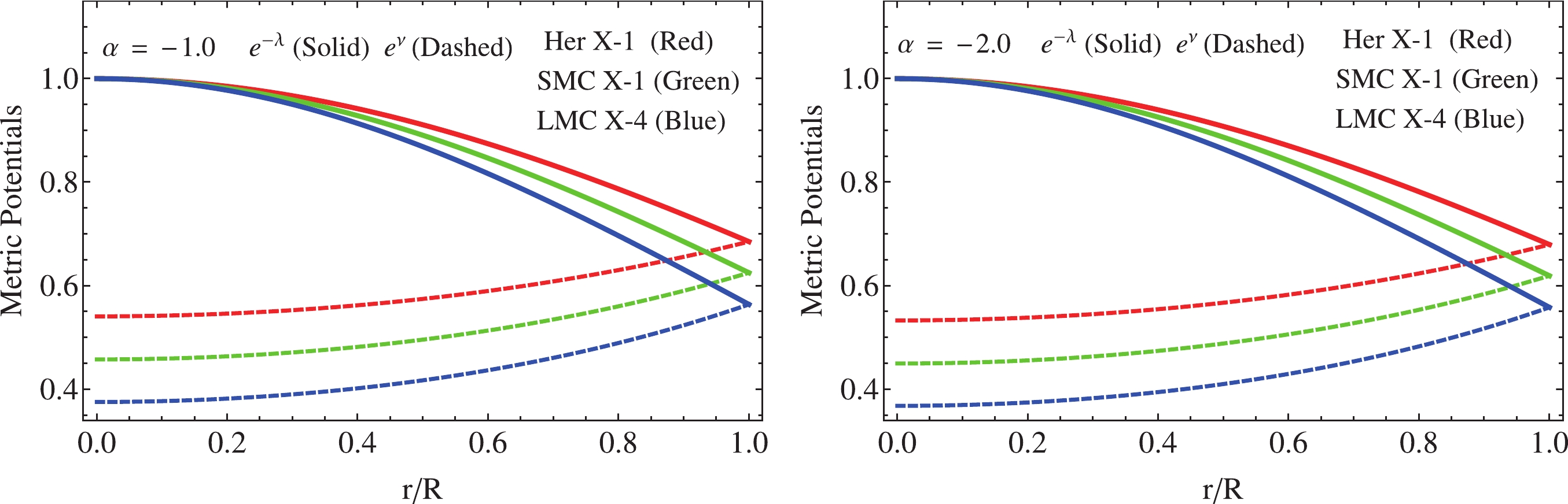
We also can observe, in Fig. 1, the behavior of the metric potentials $ {\rm e}^{-\lambda} $ and $ {\rm e}^{-\nu} $ against the radial coordinate, for the parameters involved. At this stage we have the full thermodynamic and geometric description of our model. Next, we explore all the main physical properties that this toy model must fulfill in order to represent compact configurations such as neutron stars, at least from the theoretical viewpoint.

Figure 1.  (color online) Variation of metric potentials with respect to the dimensionless radial coordinate $ r/R $, for different values of the constant parameters mentioned in Tables 2 and 5.

A well-behaved compact structure, describing real celestial bodies, must satisfy certain general requirements to achieve an appropriate model. To check these formalities, we explore here in some detail the conduct of the main salient features obtained in the previous section, namely the effective energy-density, the tangential and radial pressures, the anisotropy factor, and the geometry of the model for all r ranges, starting from the center $ r = 0 $, up to the boundary $ r = R $. Thus, regarding the interior manifold, it is observed from Eq. (42) that the pair of metric functions $ \{{\rm e}^{\nu},{\rm e}^{\lambda}\} $ is completely regular for $ r\in[0,R] $. Moreover, $ {\rm e}^{\nu}|_{r = 0}>0 $, $ \left({\rm e}^{\nu}\right)^{\prime}|_{r = 0} = 0 $ and $ {\rm e}^{\lambda}|_{r = 0} = 1 $. As we will see later, this behavior allows matching of the inner geometry to the exterior spacetime in a smooth way at the interface $ \Sigma\equiv r = R $ to realize the constant parameters that characterize the model. Meanwhile, not only the geometry must be well-behaved for the interval $ 0\leqslant r \leqslant R $. In this regard, the main thermodynamic variables must respect some criteria. From expressions (38)–(40), at the center of the compact configuration, we have

These quantities should be monotonous decreasing functions from the center toward the surface of the star; consequently, their maximum values must be attained at $ r = 0 $. Moreover, these observables must be positive everywhere inside the structure. Thus, from (44), the following is obtained

Furthermore, the equation of state parameter $ \omega\equiv p_{r}/\rho\leqslant 1 $ leads to

Therefore, the constant parameter B is restricted to lay between

The monotonous decreasing behavior of these physical quantities means that they all reach their minimum values at the surface $ \Sigma $. In Fig. 2, the trends of the effective radial and tangential pressures are depicted. It is observed that both the pressure waves in the principal direction of the object coincide at the center. Additionally, the pressure waves in the tangential direction $ p_{t} $ dominate those that are radial $ p_{r} $ at every point inside the star. Furthermore, the effective radial pressure is totally vanishing at the boundary $ \Sigma $. The trace of the effective energy-density $ \rho $ is illustrated in the lower row (right panel) of Fig. 2. As can be appreciated, its behavior respects the guidelines discussed above for stellar interiors.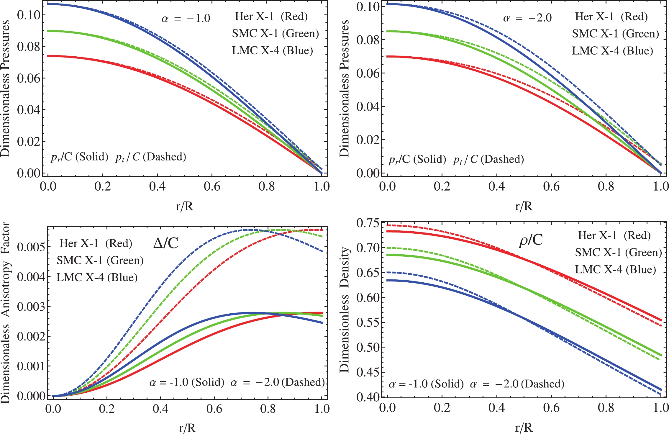

Figure 2.  (color online) Upper panels: The radial $ p_{r} $ and tangential $ p_{t} $ pressures against $ r/R $. Lower left panel: the anisotropy factor $ \Delta $ against the dimensionless radius. Lower right panel: The energy-density versus the ratio $ r/R $. These plots were obtained by using different values of constant parameters depicted in Tables 2 and 5.

As compact objects are delimited for the boundary $ \Sigma\equiv r = R $, the material content threading the stellar interior must be confined between $ 0 $ and R. To ensure the confinement of this matter distribution, the so-called junction conditions must be investigated at the surface of the structure. In general relativity theory, this procedure is performed by applying the well known Israel-Darmois [103, 104] matching conditions. To achieve this, the inner manifold $ {{\cal{M}}^{-}} $ describing the stellar interior is matched in a smooth way at the interface $ \Sigma $ with the corresponding exterior manifold $ {{\cal{M}}^{+}} $. Here, the outer spacetime is described by the vacuum Schwarzschild solution [105]

The above spacetime (48) is pertinent because the present model represents an uncharged anisotropic solution. Nevertheless, this could involve a more complicated situation due to the modifications introduced in the geometry and material parts by the $ \theta $-sector. In principle, the new source $ \theta_{\mu\nu} $ could modify the exterior geometry as well as its material content. If this is the case, the outer manifold (48) becomes

where $ g(r) $ represents the deformation function (see [71] and references therein for further details). In this regard, the minimally deformed Schwarzschild spacetime has been analyzed in [70]. Here, and without loss of generality, we shall assume that $ g(r) = 0 $, i.e., the exterior manifold surrounding the stellar interior is the original vacuum Schwarzschild solution. Therefore, the compliance of the matching conditions at the interface $ \Sigma $ dictates the continuity of the first and second fundamental forms. At the hyper-surface described by $ \Sigma $, the inner $ {{\cal{M}}}^{-} $ and outer $ {{\cal{M}}}^{+} $ manifolds induce the intrinsic and extrinsic curvatures characterized by the metric tensor $ g_{\mu\nu} $ and the symmetric extrinsic curvature tensor $ K_{ij} $ (Latin indices run over spatial coordinates only), respectively. Given that the metric tensor $ g_{\mu\nu} $ is continuous across the surface $ \Sigma $, we have, from Eqs. (42) and (48),

In the expressions (50)–(51), the quantity $ {M} $, which corresponds to the total mass contained by the fluid sphere, replaces the Schwarzschild mass $ \tilde{M} $ because at the boundary $ \Sigma $, both quantities coincide, i.e., $ m(r)|_{r = R} = M = \tilde{M} $. Meanwhile, the object $ K_{ij} $, which determines the continuity of the components of the second fundamental form, is guaranteed only in the case where the surface is free from thin shells or surface layers [103]. In such a case, the $ r-r $ component of $ K_{ij} $ leads to

Thus, the condition $ p_r(R) = 0 $ entails that there are no thin shells. Consequently, the surface density $ \sigma $ and pressure $ \cal{P} $ [103] induced on the boundary are completely vanished; thus, the extrinsic curvature tensor is continuous. To guarantee a null radial pressure at the boundary, from Eq. (52), one obtains the following relation to determine the constant B,

The continuity of $ K_{\theta\theta} $ and $ K_{\phi\phi} $ yields

where M is the total mass contained by the fluid sphere. It should be noted that expression (51) is completely equivalent to expression (54) (for more details see appendix A). Then, Eqs. (50), (51), and (53) are the necessary conditions to obtain all the constant parameters. As follows, we shall fix $ \alpha $, C, and the radius R. In Table 1, the obtained mass and parameters A and B are displayed.

Strange Stars Candidates	$M_{GR}/M_{\odot}$	$R /{\rm{km} }$	$u_{GR}=M_{GR}/R$	$z_{s}$	$M/M_{\odot}$	$u=M/R$	$z_{s}$(MGD)
${\rm{Her}}\ X-1$ [96]	$0.85$	$8.1$	$0.154595$	$0.203153$	$0.87$	$0.157403$	$0.208073$
${\rm{SMC}}\ X-1$ [97]	$1.04$	$8.301$	$0.184571$	$0.259026$	$1.06$	$0.187469$	$0.264848$
${\rm{LMC}}\ X-4$ [97]	$1.29$	$8.831$	$0.215199$	$0.324997$	$1.31$	$0.218044$	$0.331663$

Table 1.  The numerical values for the total mass, compactness factor and surface gravitational red–shift for $ a = -1 $, $ b = 4 $ and $ \alpha = -1.0 $.

In this section, the most important results obtained in this work are discussed and highlighted. These results concern the obtained inner geometry describing the stellar interior, and the behavior of the principal thermodynamic observables, such as density $ \rho $, radial pressure $ p_{r} $, and tangential pressure $ p_{t} $. Besides, the energy conditions and the equilibrium and stability mechanism are analyzed to verify if the model could represent compact structures such as neutron or quark stars.

We start the discussion by analyzing the obtained geometry given by Eq. (42). As can be seen, the deformation function $ f(r) $ (34) is vanishing at the center of the star $ r = 0 $ and completely regular at every point inside the structure. This fact ensures that the deformed metric potential $ {\rm e}^{-\lambda}\mapsto \mu(r)+\alpha f(r) $ matches with the result obtained in general relativity, i.e., $ {\rm e}^{\lambda(r)}|_{r = 0} = 1 $ as expected. The trend of both metric potentials is depicted in Fig. 1 for $ \alpha = -1.0 $ (left panel) and $ \alpha = -2.0 $ (right panel). The solid line represents the inverse of the radial metric potential $ {\rm e}^{-\lambda} $ while the dashed line represents the temporal potential $ {\rm e}^{\nu} $. As illustrated in Fig. 1, the temporal component of the interior spacetime respects the pertinent requirements, that is, monotonous increasing function with increasing radial coordinate and $ {\rm e}^{\nu(0)}>0 $ at $ r = 0 $. Additionally, both metric potentials coincide at the boundary of the compact structure. This shows that the junction condition process is correct.

The principal thermodynamic variables driving the matter distribution inside the fluid sphere are shown in Fig. 2. As can be seen in Fig. 2 (upper panels), the radial and tangential pressures coincide at the center of the structure and drift apart toward the boundary. Moreover, the transverse pressure dominates the radial one in all cases. It is worth mentioning that the central pressure increases with increasing mass. Furthermore, from Fig. 2 (lower left panel), it is clear that the anisotropy quantifier $ \Delta $ is a monotonous increasing function with increasing radius. Of course, as can be seen at the center of the object, we have $ \Delta = 0 $ because at $ r = 0 $, both pressures are equal. However, at the surface of the star, the blue curve takes greater values compared with the red and green curves. Thus, the difference between $ p_{r} $ and $ p_{t} $ increases as the total mass increases. At this point, it should be noted that in order to have a positive anisotropy factor $ \Delta $ inside the stellar interior, from Eq. (41) is evident that $ \alpha $ must be negative. As recognized by Gokhroo and Mehra, a positive anisotropy factor allows the construction of more compact objects [19]. With respect to the energy–density $ \rho $ from the lower right panel of Fig. 2, it can be seen that in all cases, this observable takes its upper value at the center of the star and decreases monotonically toward the boundary $ \Sigma $. An interesting point to be highlighted here is that the central parameters $ \rho(0) $ and $ p_{r}(0) $ and the surface density $ \rho(R) $ increase with increasing mass and increasing $ \alpha $ magnitude (for further details see Tables 3 and 6). Meanwhile, as shown in Table 7, the central and surface density values in the GR case are dominant when MGD is present, while GR central pressure dominates the MGD scenario. Next, in the upper left ($ \alpha = -1.0 $) and right ($ \alpha = -2.0 $) panels of Fig. 3, the velocities of the pressure waves in the main directions are illustrated, expressed by

Strange Stars Candidates	$\rho(0)$$\times 10^{15}/({\rm{g} }/{\rm{cm} }^{3})$	$\rho(R)$$\times 10^{14}/({\rm{g} }/{\rm{cm} }^{3})$	$p_{r}(0)$$\times 10^{35}/({\rm{dyne} }/{\rm{cm} }^{2})$	$\Gamma_{{\rm{crit}}}$	$\Gamma$
${\rm{Her}}\ X-1$ [96]	$0.91838$	$6.94944$	$0.83461$	$1.47575$	$3.87767$
${\rm{SMC}}\ X-1$ [97]	$1.08795$	$7.68708$	$1.28333$	$1.50295$	$3.18179$
${\rm{LMC}}\ X-4$ [97]	$1.14485$	$7.55726$	$1.73542$	$1.53061$	$2.67374$

Table 3.  The numerical values for central and surface density, central pressure, critical adiabatic index, and central adiabatic index for different values listed in Tables 1 and 2, taking $ a = -1 $, $ b = 4 $, and $ \alpha = -1.0 $.

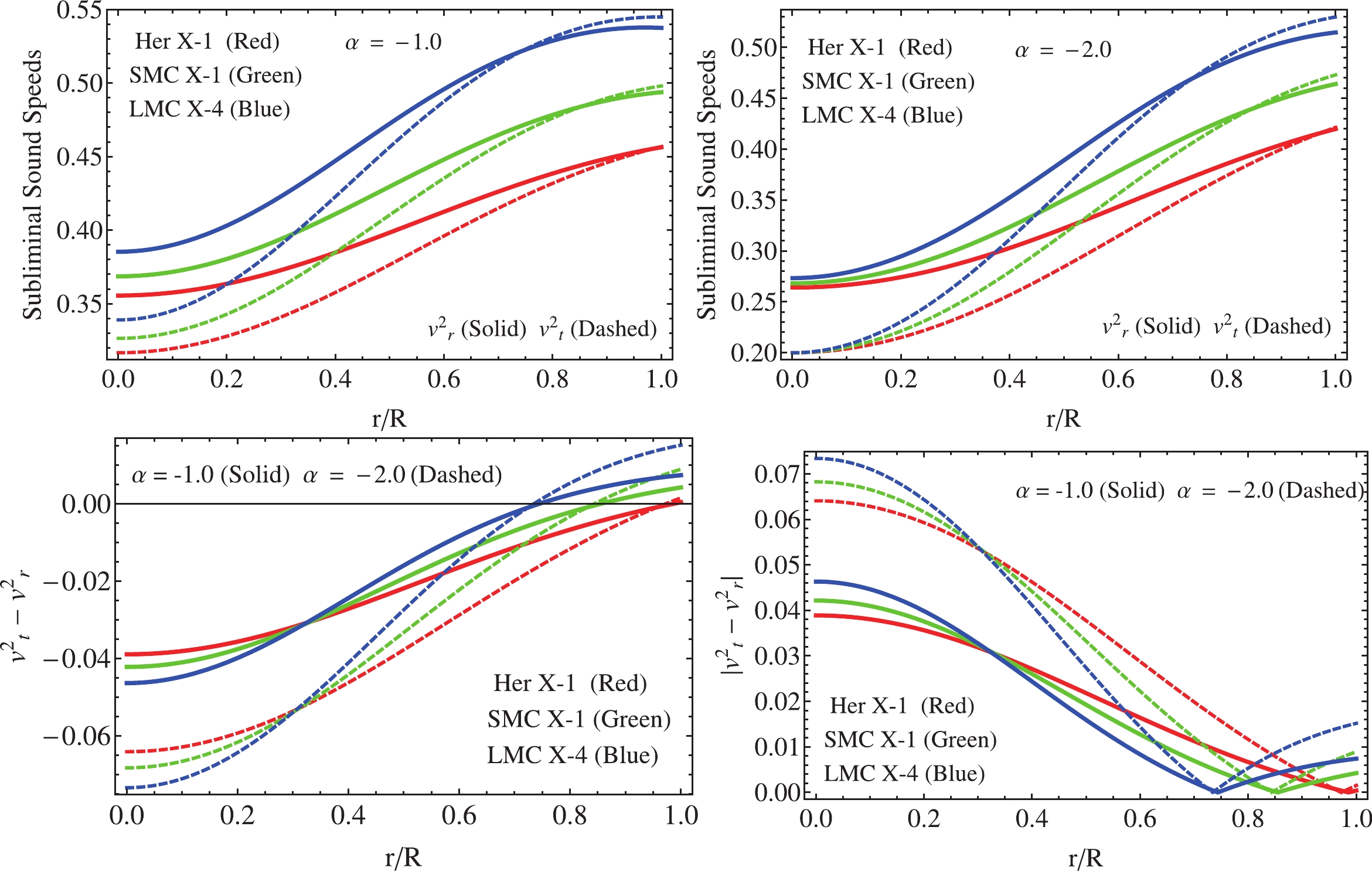
Figure 3.  (color online) Upper row: The square of sound velocity of pressure waves in the principal directions for $ \alpha = -1.0 $ (left side) and $ \alpha = -2.0 $ (right side), respectively. Lower left panel: The different of the squared sound velocities against the dimensionless radial coordinate. Lower right panel: Abreu's factor versus the radial coordinate $ r/R $.

Strange Stars Candidates	$\rho(0)$$\times 10^{15}/({\rm{g} }/{\rm{cm} }^{3})$	$\rho(R)$$\times 10^{14}/({\rm{g} }/{\rm{cm} }^{3})$	$p_{r}(0)$$\times 10^{35}/({\rm{dyne} }/{\rm{cm} }^{2})$	$\Gamma_{{\rm{crit}}}$	$\Gamma$
${\rm{Her}}\ X-1$ [96]	$0.95929$	$6.99941$	$0.81191$	$1.47828$	$3.07256$
${\rm{SMC}}\ X-1$ [97]	$1.14006$	$7.71957$	$1.24992$	$1.50557$	$2.47052$
${\rm{LMC}}\ X-4$ [97]	$1.23529$	$7.69822$	$1.73586$	$1.53318$	$2.02458$

Table 6.  The numerical values for central and surface density, central pressure, critical adiabatic index, and central adiabatic index for different values listed in Tables 4 and 5, taking $ a = -1 $, $ b = 4 $, and $ \alpha = -2.0 $.

Strange Stars Candidates	$\rho(0)$$\times 10^{15}/({\rm{g} }/{\rm{cm} }^{3})$	$\rho(R)$$\times 10^{14}/({\rm{g} }/{\rm{cm} }^{3})$	$p_{r}(0)$$\times 10^{35}/({\rm{dyne} }/{\rm{cm} }^{2})$	$\Gamma_{{\rm{crit}}}$	$\Gamma$
${\rm{Her}}\ X-1$ [96]	$0.87932$	$6.89622$	$0.85361$	$1.47321$	$5.10185$
${\rm{SMC}}\ X-1$ [97]	$1.03832$	$7.65191$	$1.31203$	$1.50033$	$4.31034$
${\rm{LMC}}\ X-4$ [97]	$1.11676$	$7.67022$	$1.81969$	$1.52804$	$3.76308$

Table 7.  The numerical values for central and surface density, central pressure, critical adiabatic index, and central adiabatic index for the GR case ($ \alpha = 0.0 $).

which are less than the unit (where $ c = 1 $); then, the present model satisfies the causality condition. Nevertheless, as the mass increases, a swap between $ v_{r} $ and $ v_{t} $ occurs. This fact corresponds with the instabilities against the cracking process [18] introduced by the anisotropies in the stellar matter distribution. To check the unstable regions inside the star, we have plotted the so-called Abreu's factor $ |v^{2}_{t}-v^{2}_{r}| $ [26] (lower right panel in Fig. 3) and the difference of the square sound velocities (lower left panel in Fig. 3). The change in sign of $ v^{2}_{t}-v^{2}_{r} $ indicates that the system presents unstable regions, i.e., zones with cracking. Explicitly, the stable/unstable regions within the stellar interior, when local anisotropies are present, can be found as [26],

Considering (56), $ 0\leqslant |v^{2}_{t}-v^{2}_{r}|\leqslant 1 $ is obtained, which can be re-expressed as follows

Therefore, the compact structure will be stable under the radial perturbations induced by local anisotropies, if the subliminal radial sound speed, $ v^{2}_{r} $, of the pressure waves dominates everywhere against the subliminal sound velocity of the pressure waves in the tangential direction $ v^{2}_{t} $. As can be seen from the lower panels in Fig. 3, there is a clear tendency of the system to present unstable regions when the mass of the system increases. Furthermore, the situation worsens when the parameter $ \alpha $ increases (in magnitude). Contrarily, for values corresponding to the star Her X–1 (the least massive star), the system does not present unstable zones. Thus, it is clear that the mass of the object directly influences the fulfillment of this stability criterion, as does the parameter $ \alpha $. Therefore, in light of the features above, one possibility to circumvent cracked areas in the stellar interior, without considering less massive objects, would be to limit the value (magnitude) of the constant coupling $ \alpha $. This can also be achieved without loss of generality. The latter is true because $ \alpha $ is a free parameter that only controls the strength of the anisotropy induced via MGD by gravitational decoupling.

Meanwhile, we have also checked the stability of the configuration using the relativistic adiabatic index $ \Gamma $. For a Newtonian isotropic fluid distribution, the stability condition is $ \Gamma>4/3 $ [7, 15]. However, in the anisotropic relativistic scenario, the above condition is quite different. In that case, the system should satisfy [16, 17]

where $ \rho_{0} $ corresponds to the initial density and $ p_{r0} $ represents the radial pressure (when the fluid is in static equilibrium). Finally, $ p_{t0} $ is the corresponding tangential pressure (again when the fluid is in static equilibrium). The second term on the right hand side represents the relativistic corrections to the Newtonian perfect fluid and the third term is the contribution due to anisotropy. It is observed that the stability condition is modified due to relativistic corrections and the presence of local anisotropies. However, as identified by Chandrasekhar [106, 107], relativistic correction to the adiabatic index could in principle introduce some instabilities within the stellar interior. This would occur in the case where the object contracts until it reaches the critical radius

where K is a constant depending on the density distribution. As expected, in this case, the local anisotropies help to avoid this situation. Moreover, a more strict condition on the adiabatic index for a stable region was recently computed in [108]. It was found that the critical value of the adiabatic index $ \Gamma_{\rm{crit}} $ (to have a stable structure) depends on the amplitude of the Lagrangian displacement from equilibrium and the compactness factor $ u\equiv M/R $. The amplitude of the Lagrangian displacement is characterized by the parameter $ \xi $, so taking particular form of this parameter, the critical relativistic adiabatic index is given by

where the stability condition becomes $ \Gamma\geqslant \Gamma_{\rm{crit}} $. Meanwhile, the explicit form to compute the adiabatic index is given by [14]

As the left panel of Fig. 4 shows, the system is completely stable from the relativistic adiabatic index point of view for all cases. In addition, as the numerical values displayed in Tables 3 ($ \alpha = -1.0 $) and 6 ($ \alpha = -2.0 $) corroborate the condition, $ \Gamma\geqslant \Gamma_{\rm{crit}} $ is satisfied in all cases. It should be noted that as the mass of the object and the magnitude of $ \alpha $ increase, the central value of $ \Gamma $ decreases. Furthermore, as Table 7 shows, when $ \alpha = 0.0 $ (GR case), the adiabatic index takes higher values at $ r = 0 $, indicating, as Chandrasekhar argued, that the presence of anisotropy does not always improve the stability conditions of the system. However, despite this, the system is stable under this criterion. In a broader context, discussing stability mechanisms is rather heuristic; therefore, there are many ways to check or analyze the stability of a system under radial perturbations caused by the presence of anisotropies. Recently, in [109], the convection stability concept was introduced. In short, a stellar interior is stable against convection when a fluid element displaced downward floats back to its initial position. This occurs whenever $ \rho^{\prime\prime}<0 $. In Fig. 4 (middle panel) it is shown that the model is unstable after undergoing convection motion. As in the relativistic adiabatic index case, there is a clear tendency of the system to reduce the stability when both M and $ \alpha $ increase in magnitude. As can be noted, for the less massive star (Her X–1) and $ \alpha = -1.0 $, the system is stable under this approach, while the other cases are not. Furthermore, the same situation occurs when Abreu's criterion analysis is employed, i.e., the system seems to become unstable as the mass increases. On the other hand, a more reliable and well posed stability criterion is based on the well–known Harrison–Zeldovich–Novikov [110, 111] procedure. This criterion states that any fluid configuration is stable if the mass is an increasing function with respect to the central density $ \rho(0) = \rho_{c} $ i.e., $ \frac{\partial M(\rho_{c})}{\partial \rho_{c}}>0 $; otherwise, the model is unstable. As the right panel in Fig. 4 depicts, the total mass as a function of the central density is an increasing quantity. Therefore, the present model is completely stable.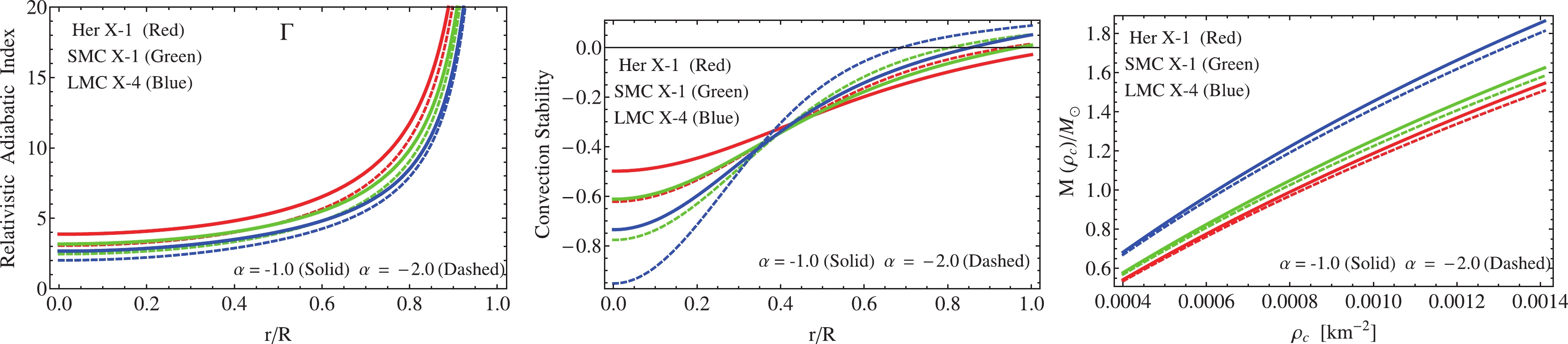

Figure 4.  (color online) Left panel: Variation of the adiabatic index $ \Gamma $ versus $ r/R $. Middle panel: The convection stability factor against the dimensionless radius $ r/R $. Right panel: The variation of the total mass against the central density.

The balance of the system under different forces, such as gravitational force $ F_{g} $, hydrostatic force $ F_{h} $, and anisotropic force $ F_{a} $, is studied by employing the conservation law of the energy-momentum tensor $ \nabla_{\mu}T^{\mu\nu} = 0 $ which yields [63]

Expression (62) can be seen as a generalization of the well-known Tolman–Oppenheimer–Volkoff (TOV) limit [1, 112], which describes the hydrostatic equilibrium of isotopic fluid distributions. In this case, we are dealing with an anisotropic fluid sphere where the corresponding modifications are encoded into the $ \theta $-sector. A closer look at equation (62) reveals that the hydrostatic, gravitational, and anisotropy gradients are given by

It is observed that gravitational decoupling by MGD modifies the usual gradients, i.e., the hydrostatic and gravitational, introducing an extra factor moderated by the dimensionless parameter $ \alpha $. This new component $ F_{a} $ plays the role of the anisotropic gradient, where if $ F_{a}>0 $, the system experiences a repulsive force counteracting, with the help of $ F_{h} $, the gravitational force $ F_{g} $ to avoid the gravitational collapse of the structure onto a point singularity. It should be noted that in the limit $ \alpha\rightarrow0 $, the TOV equation is recovered. As Fig. 5 illustrates, the system is in equilibrium under the aforementioned forces. Notwithstanding, notice that the anisotropic force is negligible in all cases compared with the hydrostatic and gravitational forces. Despite its small contribution, the anisotropic force helps to counteract the gravitational gradient, allowing the system to remain balanced against gravitational collapse.

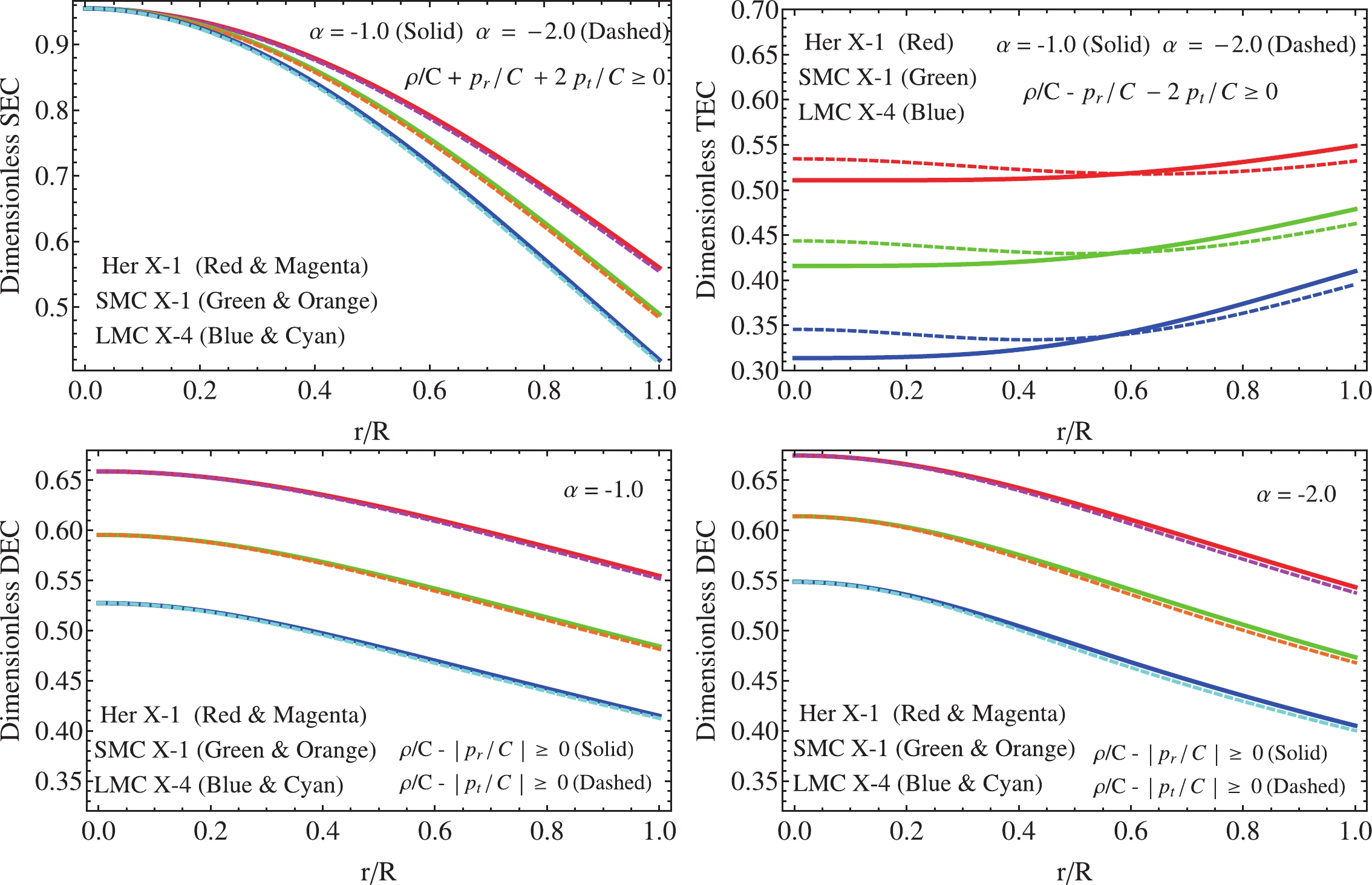
Figure 5.  (color online) The Tolman-Oppenheimer-Volkoff equation versus $ r/R $, representing the balance of the system under the gravitational, hydrostatic and anisotropic forces.

To verify if the energy-momentum tensor threading the material content within the star is well-defined, there are some conditions that are suitable to satisfy in order to obtain a well-defined physical system. These are refereed as energy conditions, specifically they are: i) the weak energy condition (WEC), ii) the null energy condition (NEC), iii) the dominant energy condition (DEC), iv) the strong energy condition (SEC), and finally v) the trace energy condition (TEC). Explicitly, these are given by [113]

where the sub-index i represents radial r or transverse t, respectively; whereas $ \; t^\mu $ and $ l^\mu $ are the time-like vector and null vector, respectively. In principle, the origin of the above inequalities come from purely geometric equations, namely the Raychaudhuri equations [114]. The Einstein field equations relate the geometry of the spacetime $ R_{\mu\nu} $ with the matter content $ T_{\mu\nu} $. In addition, the Raychaudhuri equations can be combined to obtain the above inequalities. In Fig. 6, it is clear that the SEC (upper left panel) and DEC (lower panels) are satisfied for all points within the compact object. Moreover, as inequalities (66)–(70) show, the WEC is implied by the DEC, and the NEC by the SEC. Besides, $ \rho $, $ p_{r} $, and $ p_{t} $ are strictly positive functions in the range $ 0\leq r\leq R $, which ensure the fulfilment of the NEC and WEC, so we can conclude that the energy-momentum tensor threading the matter distribution of the fluid sphere is well-behaved and represents an admissible physical fluid. Furthermore, the TEC condition is also satisfied, as depicted in the upper right panel in Fig. 6.

Figure 6.  (color online) Upper row: The strong energy condition (SEC) and trace energy condition (TEC) versus the dimensionless distant $ r/R $. Lower row: The dominant energy condition (DEC) for different values exhibited in Tables 2 and 5.

Inclusion of an extra component $ \theta_{\mu\nu} $ into the matter sector via a dimensionless parameter $ \alpha $ alters many important properties of the compact structures. Indeed, the linear mapping expressed by Eq. (21), introduced in the formalism to separate the seed source from the new factor, naturally induces a modification of the gravitational mass definition. As usual, by integrating the temporal component of the Einstein field equations (10), one obtains

However, considering (16) and (21), Eq. (71) becomes

Hence, one can rewrite the mass function (72) as

that is, the gravitational mass can be understood as the usual gravitational GR mass plus a contribution from the MGD process. It is clear from (73) that more massive compact objects can be obtained when MGD is present if $ f(r)>0 $ and $ \alpha<0 $ (and vice versa), for all $ r\in[0,R] $. In this case, as realized before, $ \alpha $ must be negative to ensure a positive anisotropy factor. Moreover, the expression for the decoupler function $ f(r) $ given by (33) shows that $ f(r) $ is a strictly positive defined quantity. Additionally, the compactness factor u also changes, as

Again $ \alpha = 0 $ regains the GR case; as the seed solution is isotropic, the mass–radius ration is bounded by the well-known Buchdhal limit [115]. In a more general context, the inclusion of new fields [116] and anisotropies [117] modified the mentioned limit. In this sense, it is possible to include the so-called extra packing of mass [118] in the framework of gravitational decoupling by MGD. As Tables 1 and 4 display, the total gravitational mass M and mass–radius ratio u are greater than their GR counterparts, and as $ \alpha $ increases in magnitude, the mentioned macro physical parameters also increase in magnitude. This is because these observables have a linear dependence in $ \alpha $. The surface gravitational redshift $ z_{s} $ is closely related with these observables. In fact, $ z_{s} $ is defined as follows

Strange Stars Candidates	$M_{GR}/M_{\odot}$	$R/{\rm{km} }$	$u_{GR}=M_{GR}/R$	$z_{s}$	$M/M_{\odot}$	$u=M/R$	$z_{s}$(MGD)
${\rm{Her}}\ X-1$ [96]	$0.85$	$8.1$	$0.154595$	$0.203153$	$0.88$	$0.160209$	$0.21305$
${\rm{SMC}}\ X-1$ [97]	$1.04$	$8.301$	$0.184571$	$0.259026$	$1.07$	$0.190366$	$0.27075$
${\rm{LMC}}\ X-4$ [97]	$1.29$	$8.831$	$0.215199$	$0.324997$	$1.32$	$0.220889$	$0.33843$

Table 4.  The numerical values for the total mass, compactness factor, and surface gravitational red–shift for $ a = -1 $, $ b = 4 $, and $ \alpha = -2.0 $.

Tables 1 and 4 depict the corresponding values of this important astrophysical observable in the GR and MGD scenarios, respectively. In this direction, Ivanov [119] pointed out that for any spherically symmetric anisotropic fluid sphere whose transverse pressure $ p_{t} $ satisfies the SEC, the surface gravitational redshift has an upper limit given by $ z_{s} = 3.842 $, whereas if $ p_{t} $ responds to the DEC, then the upper limit is $ z_{s} = 5.211 $. Here, the tangential pressure satisfies both the SEC and DEC; then, $ z_{s} $ is constrained by $ 5.211 $. As can be seen, the resulting values are within the mentioned range. In Fig. 7, the trends of M, u, and $ z_{s} $ are shown versus the dimensionless radial coordinate $ r/R $. Meanwhile, to study the stiffness of the equation of state (30) relating the components of the$ \theta $–sector, we plotted the M–R curve for the different values given in Tables 1, 2, 4, and 5 corresponding to the strange star candidates Her X–1, SMC X–1, and LMC X–4 (see Fig. 8). Table 8 shows the corresponding numerical data extracted from Fig. 8. It is observed that for the constant parameters obtained for the mentioned compact stars, the maximum mass overcomes the established limit for neutron and quark stars, i.e., $ M = 2M_{\odot} $. Nevertheless, as $ \alpha $ increases in magnitude, the maximum mass decreases. Meanwhile, the compactness factor remains bounded by the Buchdahl limit $ 4/9 $. This fact is very important, as it states that the system will not undergo a gravitational collapse. With respect to radius R, the reported values obtained from Fig. 8 are within the branch of neutron stars [96, 97]. The values of the surface gravitational redshift are bounded by $ 5.211 $. Moreover, these values are within the scope of the reported numerical data in [100-102] for the same model.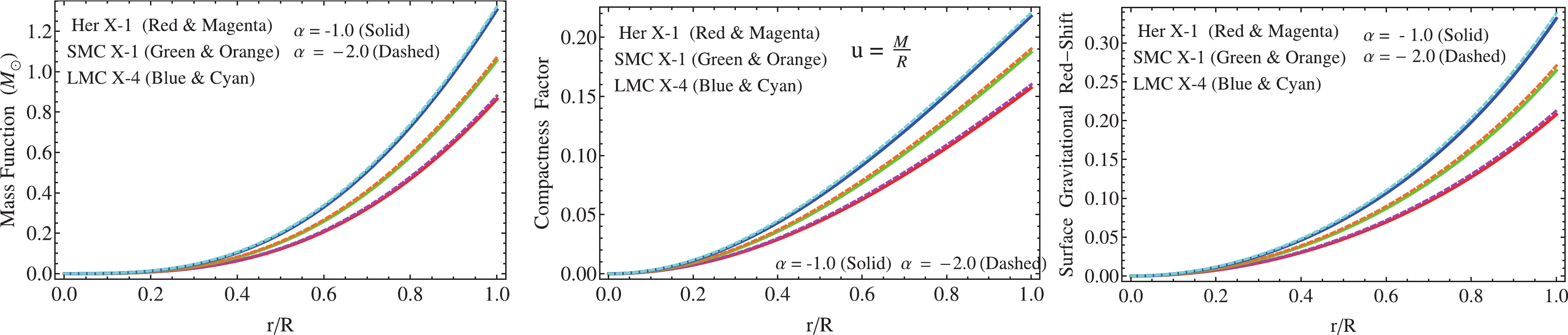

Figure 7.  (color online) Left panel: The mass function versus $ r/R $. Middle panel: The mass–radius ratio versus the dimensionless radius $ r/R $. Right panel: The trend of the surface gravitational red–shift versus $ r/R $.

Strange Stars candidates	$C /{\rm{km} }^{-2}$	$A$ (Dimensionless)	$B$ (Dimensionless)
${\rm{Her}}\ X-1$ [96]	$0.0009287$	$0.5408387$	$-2.4614406$
${\rm{SMC}}\ X-1$ [97]	$0.0011763$	$0.4576442$	$-2.0636227$
${\rm{LMC}}\ X-4$ [97]	$0.0013375$	$0.3754957$	$-1.6360451$

Table 2.  The numerical values of constant parameters C, A, and B for different values of M and R mentioned in Table 1, and $ a = -1 $, $ b = 4 $, and $ \alpha = -1.0 $.

Strange Stars candidates	$C /{\rm{km} }^{-2}$	$A$ (Dimensionless)	$B$ (Dimensionless)
${\rm{Her}}\ X-1$ [96]	$0.0009545$	$0.5329893$	$-2.3111014$
${\rm{SMC}}\ X-1$ [97]	$0.0012081$	$0.4497442$	$-1.9302915$
${\rm{LMC}}\ X-4$ [97]	$0.0014077$	$0.3680033$	$-1.5194916$

Table 5.  The numerical values of constant parameters C, A, and B for different values of M and R mentioned in Table 4 and $ a = -1 $, $ b = 4 $, and $ \alpha = -2.0 $.

Figure 8.  (color online) Variation of the total mass M against the radius R, for different values of the constant parameters mentioned in Tables 1, 2, 4, and 5.

$\alpha$	$M_{{\rm{max}}}/M_{\odot}$	$R/{\rm{km} }$	$u=M_{{\rm{max}}}/R$	$z_{s}$
$-1$	2.690	11.5	0.344601	0.793747
$-1$	2.591	11.1	0.343879	0.789593
$-1$	2.487	11.0	0.333077	0.730720
$-2$	2.660	11.3	0.346789	0.806511
$-2$	2.553	11.2	0.335810	0.745066
$-2$	2.455	11.0	0.328791	0.708922

Table 8.  The numerical values for the maximum mass, radius, compactness factor and surface gravitational red–shift obtained from Fig. 8 for $ a = -1 $, $ b = 4 $, different values of $ \alpha $, and values mentioned in Tables 2 and 5.

In the present manuscript, we have investigated in detail Durgapal's fourth model in light of the MGD approach by gravitational decoupling. To achieve this, we utilized a general equation of state for the anisotropic sector and, for concrete values of the parameters a and b, we computed the corresponding deformation function as well as the components of the $ \theta_{\mu \nu} $ tensor, finally obtaining the corresponding effective fluid parameters. Furthermore, considering that the density and the radial pressure should be a monotonously decreasing function from the center toward the surface of the star, we bounded the parameter B of the modified solution. This parameter plays an important role in the original solution because preservation of the causality condition within the stellar interior depends on the magnitude and sign of this parameter. In this case, the lower and upper bounds of B are altered by the presence of $ \alpha $. Thus, the choice of $ \alpha $ is constrained to satisfy the causality condition. This fact is preserved if and only if B takes negative values. The behavior of the thermodynamic observables was studied for different values of the parameters involved in the model. As can be seen in Fig. 2, the trend of these variables is well-behaved inside the star. Besides, to ensure a well-posed stellar interior, the parameter $ \alpha $ must be negative. In Tables 3 and 6, the central density, surface density, and central pressure are shown. As can be seen, the first two increase with increasing mass and $ \alpha $ (in magnitude), whereas the central pressure decreases in magnitude. Meanwhile, Table 7 displays the same parameters for the GR case, i.e., $ \alpha = 0 $. The stability of the system was checked using different approaches: i) subliminal sound speeds of the pressure waves, ii) relativistic adiabatic index, iii) convection, and iv) the Harrison–Zeldovich–Novikov criteria. In considering i) and iii), the system presents instabilities for massive objects; in contrast, when ii) and iv) are used, the system is stable for all cases under consideration (for further details see Figs. 3 and 4). The stability analysis is very important as it determines whether the hydrostatic equilibrium under different gradients is stable or not. In this case, the present model is under hydrostatic balance produced by the hydrostatic $ F_{h} $, gravitational $ F_{g} $, and anisotropic $ F_{a} $ gradients. Fig. 5 shows the trend of these gradients along the compact structure. The positive nature of the anisotropic force $ F_{a} $ induced by MGD helps $ F_{h} $ to counteract the gravitational attraction in order to avoid the collapse of the compact configuration onto a point singularity. It is clear from the panels displayed in Fig. 5 that the anisotropic gradient increases in magnitude when $ \alpha $ increases in magnitude. Although the model satisfies the above criteria, it is also important to check the behavior of the full energy–momentum tensor inside the compact object. Regarding this, we studied the classical energy conditions, finding that the energy–momentum tensor representing the matter distribution for this toy model is completely regular and positively defined everywhere. As Fig. 6 illustrates, the SEC, DEC, and TEC are satisfied.

Contrarily, the effects induced by gravitational decoupling by the MGD scheme were explored. Here, it is evident that the map (21) alters the usual gravitational mass definition, as shown by Eq. (73). Disturbances on the gravitational mass definition yield modifications of the mass–radius ratio and surface gravitational redshift. Under this particular model, to produce more massive and compact objects, the following are necessary: $ f(r)>0 $ and $ \alpha<0 $. As can be seen in Tables 1 and 4, the mentioned parameters within the arena of MGD overcome their similes in the GR background. The affections on these important astrophysical parameters is quite relevant as, by comparison, the numerical values obtained in the GR case under the isotropic condition can be distinguished from their anisotropic counterparts when local anisotropies induced by the MGD grasp are present. In Fig. 7 the gravitational mass function, compactness factor, and surface gravitational redshift are shown. Furthermore, to examine the stiffness of the equation of state (30) employed to determine the decoupler function $ f(r) $, we built M–R plot 8 for the numerical data obtained for: Her X–1, SMC X–1 and LMC X–4 reported in Tables 1, 2, 4, and 5. As can be observed from Fig. 8, for both cases $ \alpha = -1.0 $ and $ \alpha = -2.0 $, the maximum mass and radius are $ \{2.69M_{\odot},11.5\ [{\rm km}]; 2.66M_{\odot},11.3 \ [{\rm km}]\} $, respectively (see Table 8 for more details). These results show that the maximum mass is above the limit $ M = 2M_{\odot} $ for neutron and quark stars. However, the compactness factor and redshift are within the scope of the usual numerical data. In this regard, it is worth mentioning that the maximum compactness factor remains bounded by the well-known Buchdahl limit. As a final remark, it can be concluded that the present toy model is able to represent and describe, at least from the theoretical viewpoint, relativistic anisotropic compact structures.

F. Tello–Ortiz acknowledges financial support by CONICYT PFCHA/DOCTORADO-NACIONAL/2019-21190856 and projects ANT–1756 and SEM 18–02 at Universidad de Antofagasta, Chile. F. Tello-Ortiz thanks the PhD program Doctorado en Física mención en Física Matemática de la Universidad de Antofagasta, Chile. Á. R. acknowldeges DI-VRIEA for financial support through Proyecto Postdoctorado 2019 VRIEA-PUCV. P. B. is thankful to IUCAA, Pune, Government of India for providing visiting associateship. Y. Gomez-Leyton acknowledges financial support by CONICYT PFCHA/DOCTORADO-NACIONAL/2020−21202056.

In this appendix, we will demonstrate that Eqs. (51) and (54) are completely equivalent in order to determine the total mass M contained by the fluid sphere. Hence, the starting point is the field equation (10)

where, as Eq. (16) expresses, $ \rho $ is given by

and as MGD dictates (see Eq. (21)), $ {\rm e}^{-\lambda} $ reads

Next, by substituting (A2) and (A3) into (A1),

where the left-hand side can be reorganized as follows

Now, integrating both sides of (A5) over the volume $ {\rm d}V\equiv4\pi r^{2}{\rm d}r $ with $ r\in[0,R] $ and applying the first fundamental theorem of calculus, one obtains

Meanwhile, from Eq. (51)

after some algebra, the mass M is obtained as follows

where

Therefore, as can be seen, Eqs. (51) and (54) lead to the same expression to compute the total mass M inside the compact object. As a final remark, it should be noted that $ \alpha = 0 $ leads to the general relativity gravitational mass definition, although as usual, the general relativity expression can be recast by rewriting $ \tilde{\rho}+\alpha\theta^{t}_{t} = \rho $ and $ \mu(r) + \alpha f(r) = {\rm e}^{-\lambda} $, i.e., by using the effective quantities. Nevertheless, it must be considered that the density $ \rho $ and metric potential $ {\rm e}^{-\lambda} $ of the solution in that appearance hide the contribution from the gravitational decoupling and MGD.

As was pointed out by Herrera et al. [120], all the spherically symmetric and static models whose matter distribution is described by an imperfect fluid (see [121] for the charged case), can be acquired from two generating functions. These two primitive generating functions $ \zeta(r) $ and $ \Pi(r) $ are given by

Then, using Eqs. (4), (41), and (B1)–(B2), the following generators are established

At this point, it should be noted that the second generator (B2) is naturally induced by gravitational decoupling by means of MGD. Thus, if $ \alpha = 0 $, the solution becomes isotropic (one recovers the seed solution in the GR arena), then (B4) is null. In this case, the generator is given only by (B1), coinciding with the results reported by Lake in [122].