


 Abstract
 HTML
HTML Reference
 Related
 PDF
PDF


-
In 2015, the LHCb collaboration observed two pentaquark candidates
$ P_c(4380) $ and$ P_c(4450) $ in the$ J/\psi p $ mass spectrum in the$ \Lambda_b^0\to J/\psi K^- p $ decays [1]. Recently, the LHCb collaboration observed a new narrow pentaquark candidate,$ P_c(4312) $ , in the$ J/\psi p $ mass spectrum with the statistical significance of$ 7.3\sigma $ ; furthermore, they confirmed the old$ P_c(4450) $ pentaquark structure, which consists of two narrow overlapping peaks$ P_c(4440) $ and$ P_c(4457) $ , with the statistical significance of$ 5.4\sigma $ [2]. The masses and widths are$ \begin{split} &P_c(4312) : M = 4311.9\pm0.7^{+6.8}_{-0.6} \;{\rm{ MeV}}\, , \, \\ &\;\;\;\;\;\;\;\;\;\;\;\;\;\;\;\;\;\;\;\;\;\Gamma = 9.8\pm2.7^{+ 3.7}_{- 4.5} \;{\rm{ MeV}} \, , \\ & P_c(4440) : M = 4440.3\pm1.3^{+4.1}_{-4.7} \;{\rm{ MeV}}\, , \, \\ &\;\;\;\;\;\;\;\;\;\;\;\;\;\;\;\;\;\;\;\;\;\;\Gamma = 20.6\pm4.9_{-10.1}^{+ 8.7} \;{\rm{ MeV}} \, , \\ &P_c(4457) : M = 4457.3\pm0.6^{+4.1}_{-1.7} \;{\rm{ MeV}} \, ,\,\\ &\;\;\;\;\;\;\;\;\;\;\;\;\;\;\;\;\;\;\;\;\;\; \Gamma = 6.4\pm2.0_{- 1.9}^{+ 5.7} \;{\rm{ MeV}} \, . \end{split} $

(1) The
$ P_c(4312) $ can be assigned to be a$ \bar{D}\Sigma_c $ pentaquark molecular state [3-18], a pentaquark state [19-23], and a hadrocharmonium pentaquark state [24].The
$ P_c(4312) $ lies near the$ \bar{D}\Sigma_c $ threshold, which leads to the molecule assignment naturally. In Ref. [18], we performed detailed studies of the$ \bar{D}\Sigma_c $ ,$ \bar{D}\Sigma_c^* $ ,$ \bar{D}^{*}\Sigma_c $ and$ \bar{D}^{*}\Sigma_c^* $ pentaquark molecular states with the QCD sum rules by carrying out the operator product expansion up to the vacuum condensates of dimension$ 13 $ in a consistent way. The prediction$ M_P = 4.32\pm 0.11\;\rm{GeV} $ for the$ \bar{D}\Sigma_c $ molecular state supports assigning$ P_c(4312) $ to be the$ \bar{D}\Sigma_c $ pentaquark molecular state with the spin-parity$ J^P = {\dfrac{1}{2}}^- $ . On the other hand, our studies based on the QCD sum rules indicate that the scalar-diquark-scalar-diquark-antiquark type pentaquark state with the spin-parity$ J^P = {\dfrac{1}{2}}^- $ has a mass of$ 4.31\pm 0.11\;\rm{GeV} $ , whereas the axialvector-diquark-axialvector-diquark-antiquark type pentaquark state with the spin-parity$ J^P = {\dfrac{1}{2}}^- $ has a mass of$ 4.34\pm 0.14\;\rm{GeV} $ , which support assigning$ P_c(4312) $ to be a diquark-diquark-antiquark type pentaquark state [23, 25, 26].$ P_c(4312) $ may be a diquark-diquark-antiquark type pentaquark state, which has a strong coupling to the$ \bar{D}\Sigma_c $ scattering states. The strong coupling induces some$ \bar{D}\Sigma_c $ components [27]. Thus, we can reproduce the experimental value of the mass of$ P_c(4312) $ in both the scenarios of the pentaquark state and pentaquark molecular state. In Ref. [28], we choose the$ [sc]_P[\bar{s}\bar{c}]_A-[sc]_A[\bar{s}\bar{c}]_P $ type tetraquark current to study the strong decays of$ Y(4660) $ with the QCD sum rules based on solid quark-hadron duality. Our calculations showed that the hadronic coupling constant$ |G_{Y\psi^\prime f_0}|\gg |G_{Y J/\psi f_0}| $ is consistent with the observation of$ Y(4660) $ in the$ \psi^\prime\pi^+\pi^- $ mass spectrum, and that it favors the$ \psi^{\prime}f_0(980) $ molecule assignment [29, 30]. A similar mechanism may exist for$ P_c(4312) $ .In this article, we tentatively assign
$ P_c(4312) $ to be the$ \bar{D}\Sigma_c $ pentaquark molecular state with the spin-parity$ J^P = {\dfrac{1}{2}}^- $ , and study its two-body strong decays with the QCD sum rules. In Ref. [31], we assigned$ Z_c(3900) $ to be the diquark-antidiquark type axialvector tetraquark state, and studied the hadronic coupling constants in the strong decays$ Z_c(3900) \to J/\psi\pi $ ,$ \eta_c\rho $ ,$ D \bar{D}^{*} $ with the QCD sum rules based on the solid quark-hadron duality by taking into account both the connected and disconnected Feynman diagrams in the operator product expansion. The method works well for studying the two-body strong decays of$ Z_c(3900) $ ,$ X(4140) $ ,$ X(4274) $ and$ Z_c(4600) $ [31-34]. Now, we extend the method to study the two-body strong decays of the pentaquark molecular state by carrying out the operator product expansion up to the vacuum condensates of dimension$ 10 $ .The article is arranged as follows: in Sec. 2, we present the comments on the QCD sum rules for the
$ \bar{D}\Sigma_c $ pentaquark molecular state; in Sec. 3, we derive the QCD sum rules for the hadronic coupling constants in the strong decays$ P_c(4312)\to \eta_c p $ ,$ J/\psi p $ ; in Sec. 4, we present the numerical results and discussions; and we conclude our report in Sec. 5. -
In this section, we present the two-point correlation function
$ \Pi(p) $ to study the mass and pole residue of the$ \bar{D}\Sigma_c $ pentaquark molecular state with the QCD sum rules,$ \Pi(p) = {\rm i}\int {\rm d}^4x {\rm e}^{{\rm i}p \cdot x} \langle0|T\left\{J(x)\bar{J}(0)\right\}|0\rangle \, ,$

(2) where the current
$ J(x) = J_{\bar{D}\Sigma_c}(x) $ ,$ J_{\bar{D}\Sigma_c}(x) = \bar{c}(x)i\gamma_5 u(x)\, \varepsilon^{ijk} u^T_i(x) C\gamma_\alpha d_j(x)\, \gamma^\alpha\gamma_5 c_{k}(x) \, ,$

(3) and i, j, k are color indices. We choose the color-singlet-color-singlet type (or meson-baryon type) current
$ J_{\bar{D}\Sigma_c}(x) $ to interpolate the$ \bar{D}\Sigma_c $ pentaquark molecular state with the spin-parity$ J^P = {\dfrac{1}{2}}^- $ [18]. For the technical details and numerical results, one can consult Ref. [18]. In the present work, we will focus on the reliability of the single pole approximation in the hadronic spectral density.At the QCD side, the correlation function
$ \Pi(p) $ can be written as$ \begin{split} \Pi(p) =& -{\rm i}\, \varepsilon^{ijk} \varepsilon^{i^{\prime}j^{\prime}k^{\prime}} \int {\rm d}^4x {\rm e}^{{\rm i}p\cdot x}\, \Big\{ -{\rm{Tr}}\left[{\rm i}\gamma_5 C_{m^\prime m}(-x) {\rm i}\gamma_5 U_{mm^\prime}(x)\right] \,{\rm{Tr}}\left[\gamma_\alpha D_{jj^\prime}(x) \gamma_\beta C U^{T}_{ii^\prime}(x)C\right] \gamma^\alpha \gamma_5 C_{kk^{\prime}}(x)\gamma_5\gamma^\beta \\ &+ {\rm{Tr}} \left[{\rm i}\gamma_5 C_{m^\prime m}(-x) {\rm i}\gamma_5 U_{mi^\prime}(x) \gamma_\beta C D^T_{jj^\prime}(x)C \gamma_\alpha U_{im^\prime}(x)\right] \gamma^\alpha \gamma_5 C_{kk^{\prime}}(x)\gamma_5\gamma^\beta \Big\} \, , \end{split} $

(4) where
$ U_{ij}(x) $ ,$ D_{ij}(x) $ , and$ C_{ij}(x) $ are the full u, d, and c quark propagators, respectively ($ S_{ij}(x) = U_{ij}(x),\,D_{ij}(x) $ ),$\quad\quad\quad\quad\quad \begin{aligned}[b] S_{ij}(x) =& \dfrac{{\rm i}\delta_{ij}\!\not\!{x}}{ 2\pi^2x^4}-\dfrac{\delta_{ij}\langle \bar{q}q\rangle}{12} -\dfrac{\delta_{ij}x^2\langle \bar{q}g_s\sigma Gq\rangle}{192} - \dfrac{{\rm i}g_sG^{a}_{\alpha\beta}t^a_{ij}(\!\not\!{x} \sigma^{\alpha\beta}+\sigma^{\alpha\beta} \!\not\!{x})}{32\pi^2x^2} -\dfrac{1}{8}\langle\bar{q}_j\sigma^{\mu\nu}q_i \rangle \sigma_{\mu\nu}+\cdots \, , \end{aligned}$

(5) $\quad\quad\quad\quad\quad \begin{split} C_{ij}(x) =& \dfrac{\rm i}{(2\pi)^4}\int {\rm d}^4k {\rm e}^{-{\rm i}k \cdot x} \left\{ \dfrac{\delta_{ij}}{\!\not\!{k}-m_c} -\dfrac{g_sG^n_{\alpha\beta}t^n_{ij}}{4}\dfrac{\sigma^{\alpha\beta}(\!\not\!{k}+m_c)+(\!\not\!{k}+m_c) \sigma^{\alpha\beta}}{(k^2-m_c^2)^2}\right.\\ &-\left. \dfrac{g_s^2 (t^at^b)_{ij} G^a_{\alpha\beta}G^b_{\mu\nu}(f^{\alpha\beta\mu\nu}+f^{\alpha\mu\beta\nu}+f^{\alpha\mu\nu\beta}) }{4(k^2-m_c^2)^5}+\cdots\right\} \, ,\\ f^{\alpha\beta\mu\nu} =&(\!\not\!{k}+m_c)\gamma^\alpha(\!\not\!{k}+m_c)\gamma^\beta(\!\not\!{k}+m_c)\gamma^\mu(\!\not\!{k}+m_c)\gamma^\nu(\!\not\!{k}+m_c)\, , \end{split} $

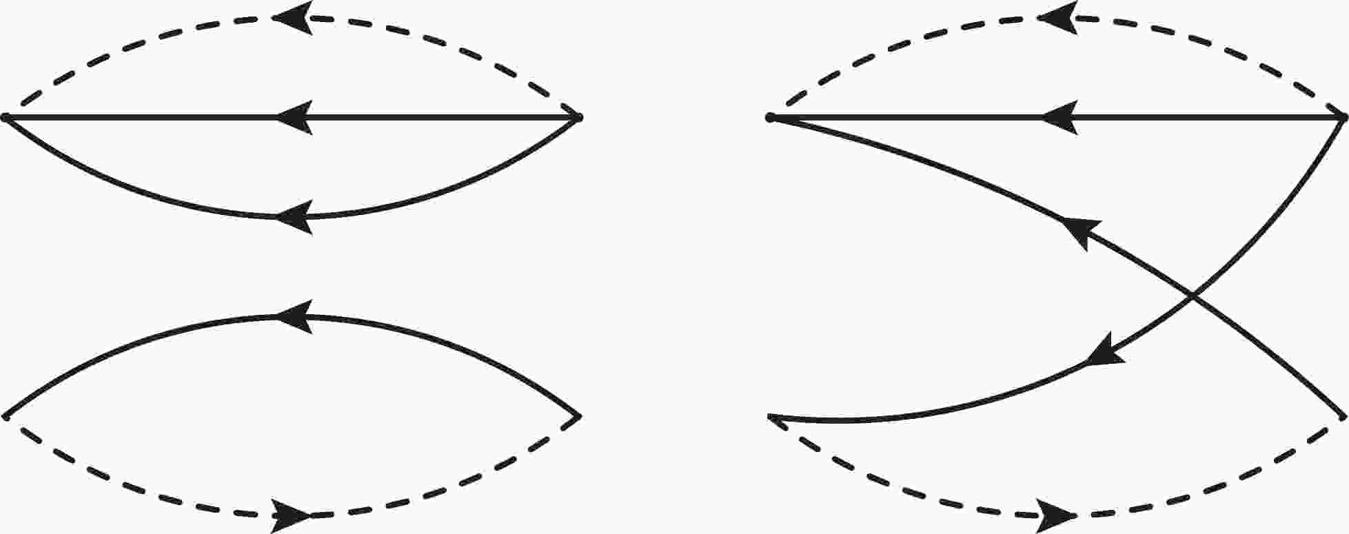
(6) $ t^n = \dfrac{\lambda^n}{2} $ ,$ \lambda^n $ is the Gell-Mann matrix [35-37].In Fig. 1, we plot two Feynman diagrams for the lowest order contributions, where the first diagram corresponds to the term with two Tr's and the second diagram corresponds to the term with one Tr in Eq. (4). The first Feynman diagram is factorizable and has the color factor
$ 18 $ , while the second Feynman diagram is non-factorizable and has the color factor$ 6 $ . In the large$ N_c $ limit$ N_c \to \infty $ , the contribution of the second Feynman diagram is greatly suppressed. In reality, the color number$ N_c = 3 $ , the second Feynman diagram plays an important role.
Figure 1. Feynman diagrams for the lowest order contributions for the baryon-meson type current
$ J(x) $ , where the solid lines and the dashed lines denote the light quarks and heavy quarks, respectively. We have taken into account the finite spatial separation between the$ \bar{c}(x)i\gamma_5 u(x) $ and$\varepsilon^{ijk} u^T_i (x) C$ $\gamma_\alpha d_j(x)\, \gamma^\alpha\gamma_5 c_{k}(x) $ clusters in the current operator$ J(x) $ .In the second Feynman diagram, we can replace the lowest order heavy quark lines and (or) light quark lines with other terms in the full propagators in Eqs. (5), (6), and obtain other non-factorizable Feynman diagrams.
In the first Feynman diagram, we can also replace the lowest order heavy quark lines and (or) light quark lines with other terms in the full propagators in Eqs. (5), (6), and obtain other factorizable Feynman diagrams. There are non-factorizable Feynman diagrams besides the factorizable Feynman diagrams, see Fig. 2. In Fig. 2, we plot the Feynman diagrams contributing to the vacuum condensates
$ \langle \bar{q}g_s\sigma G q \rangle^2 $ , which are the vacuum expectations of the quark-gluon operators of the order$ {\cal O}(\alpha_s) $ and not of the order$ {\cal O}(\alpha_s^2) $ . In Fig. 3, we plot the non-factorizable Feynman diagrams of the order$ {\cal O}(\alpha_s^2) $ from the terms with two Tr's in Eq. (4), where the first, second, third, and fourth diagrams are non-planar Feynman diagrams, while the fifth, and sixth diagrams are planar Feynman diagrams. The first and the second Feynman diagrams are suppressed by a factor$ \dfrac{1}{\sqrt{N_c}^4 }\dfrac{1}{N_c} = \dfrac{1}{N_c^3} $ in the large$ N_c $ limit compared to the first Feynman diagram in Fig. 1, while the third, fourth, fifth, and sixth diagrams are suppressed by a factor$ \dfrac{1}{\sqrt{N_c}^4 } = \dfrac{1}{N_c^2} $ . In reality, for the color number$ N_c = 3 $ , the Feynman diagrams in Fig. 3 are suppressed by a factor$ \left({\dfrac{4}{3}\dfrac{\alpha_s}{4\pi}}\right)^2\sim0.0009 $ , and play a minor role.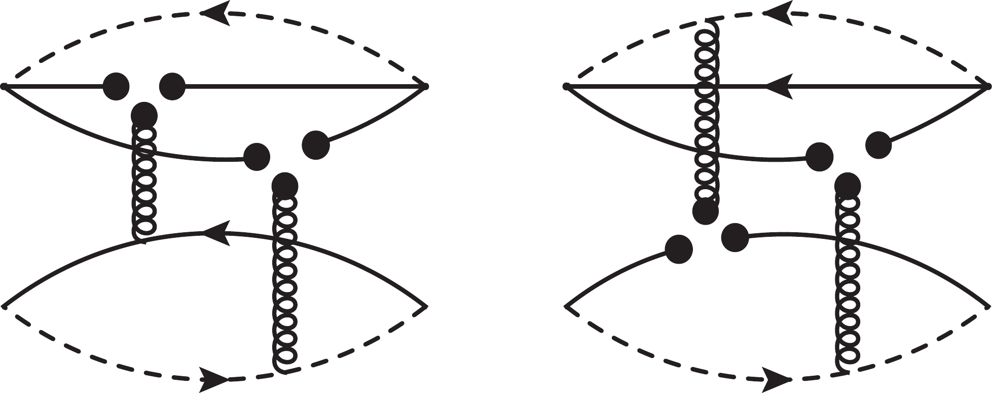
Figure 2. Non-factorizable Feynman diagrams contributing to the vacuum condensates
$ \langle \bar{q}g_s\sigma G q \rangle^2 $ from the terms with two Tr's in Eq. (4), where the solid lines and dashed lines denote the light quarks and heavy quarks, respectively. Other diagrams obtained by interchanging of the light quark lines are implied.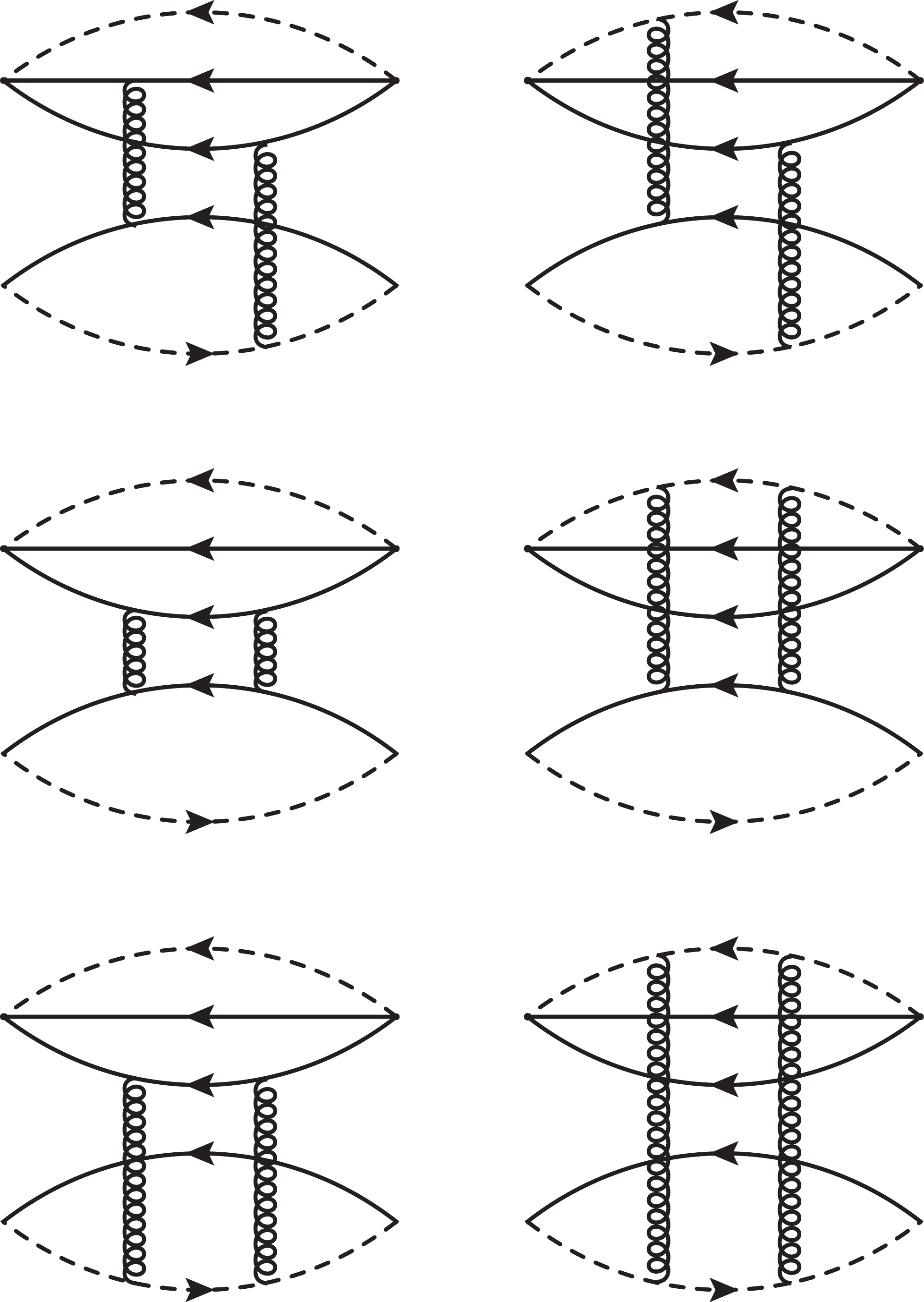
Figure 3. Non-factorizable Feynman diagrams of the order
$ {\cal O}(\alpha_s^2) $ from the terms with two Tr's in Eq. (4), where the solid lines and dashed lines denote the light quarks and heavy quarks, respectively. Other diagrams obtained by interchanging of the light and heavy quark lines are implied.In Fig. 4, we plot the non-factorizable Feynman diagrams contributing to the vacuum condensates
$ \langle \bar{q}g_s\sigma G q \rangle^2 $ for the meson-meson type currents. From the figure, we can see that the non-factorizable contributions begin at the order$ {\cal O}(\alpha_s^0) $ rather than at the order$ {\cal O}(\alpha_s^2) $ , as argued in Ref. [38]. For the nonperturbative contributions, we absorb the strong coupling constant$ g_s^2 = 4\pi\alpha_s $ into the vacuum condensates and count them as of the order$ {\cal O}(\alpha_s^0) $ .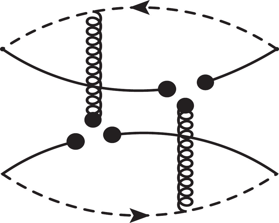
Figure 4. Non-factorizable Feynman diagrams contributing to the vacuum condensates
$ \langle \bar{q}g_s\sigma G q \rangle^2 $ for the meson-meson type currents, where the solid lines and dashed lines denote the light quarks and heavy quarks, respectively.We insist on the viewpoint that the factorizable Feynman diagrams correspond to the two-particle reducible contributions, irrespective of the baryon-meson pair or the meson-meson pair, and give the masses of the two constituent particles. Then, the attractive interactions which originate from (or are embodied in) the non-factorizable Feynman diagrams attract the two constituent particles to form the molecular states. The non-factorizable Feynman diagrams are suppressed in the large
$ N_c $ limit, which is consistent with the small bound energies of the pentaquark molecular states. The baryon-meson type or the color-singlet-color-singlet type currents couple potentially to the pentaquark molecular states.On the other hand, the baryon-meson type currents also couple to the baryon-meson pairs besides the molecular states as there exist two-particle reducible contributions. The intermediate baryon-meson loops contribute a finite imaginary part to modify the dispersion relation at the hadron side [18]. Through calculations, we observe that the zero width approximation works well, and the couplings to the baryon-meson pairs can be neglected safely.
If we only take into account the non-factorizable Feynman diagrams shown in Figs. 1 and 2, even if we obtain the stable QCD sum rules, we cannot distinguish the diquark-diquark-antiquark type substructure or the baryon-meson type substructure, and cannot select the color-singlet-color-singlet type substructure and refer to it as the molecular state. We simply obtain a hidden-charm five-quark state with the spin-parity
$ J^P = {\dfrac{1}{2}}^- $ . If we insist that it is a molecular state, then which diagram contributes to the masses of the baryon and meson constituents? In Ref. [39], the factorizable Feynman diagrams corresponding to the two-particle reducible contributions were subtracted, and only the non-factorizable Feynman diagrams were taken into account to study the pentaquark states. We do not agree with that approach. -
Here, we write down the three-point correlation functions
$ \Pi_5(p,q) $ and$ \Pi_{\mu}(p,q) $ in the QCD sum rules,$ \Pi_5(p,q) = {\rm i}^2\int {\rm d}^4x{\rm d}^4y {\rm e}^{{\rm i}p \cdot x}{\rm e}^{{\rm i}q \cdot y} \langle0|T\left\{J_5(x)J_N(y)\bar{J}(0)\right\}|0\rangle \, , $

(7) $ \Pi_\mu(p,q) = {\rm i}^2\int {\rm d}^4x{\rm d}^4y {\rm e}^{{\rm i}p \cdot x}{\rm e}^{{\rm i}q \cdot y} \langle0|T\left\{J_\mu(x)J_N(y)\bar{J}(0)\right\}|0\rangle \, , $

(8) where
$ \begin{split} &J_5(x) = \bar{c}(x){\rm i}\gamma_5 c(x)\, ,\\ &J_\mu(x) = \bar{c}(x) \gamma_\mu c(x)\, ,\\ &J_N(y) = \varepsilon^{ijk} u^T_i(y) C\gamma_\alpha u_j(y)\, \gamma^\alpha\gamma_5 d_{k}(y) \, , \\ &~~J(0) = \bar{c}(0){\rm i}\gamma_5 u(0)\, \varepsilon^{ijk} u^T_i(0) C\gamma_\alpha d_j(0)\, \gamma^\alpha\gamma_5 c_{k}(0) \, , \end{split} $

(9) and i, j, k are color indices. We choose the currents
$ J_5(x) $ ,$ J_\mu(x) $ ,$ J_N(y) $ , and$ J(0) $ to interpolate$ \eta_c $ ,$ J/\psi $ , p, and$ P_c(4312) $ , respectively. Thereafter we will denote the proton p as N to avoid confusion due to the four-momentum$ p_\mu $ .At the hadron side, we insert a complete set of intermediate hadron states with the same quantum numbers as the current operators
$ J_5(x) $ ,$ J_\mu(x) $ ,$ J_N(y) $ , and$ J(0) $ into the correlation functions$ \Pi_5(p,q) $ and$ \Pi_{\mu}(p,q) $ to obtain the hadronic representation [35, 40, 41]. After isolating the pole terms of the ground states, we obtain the following results:$\quad\quad\quad\quad\quad\quad \begin{split} \Pi_5(p,q) & = \dfrac{f_{\eta_c}m_{\eta_c}^2\lambda_P\lambda_N}{2m_c}\dfrac{-{\rm i}u(q)\,\langle\eta_c(p)N(q)|P(p^\prime)\rangle \, \bar{u}(p^\prime)}{\left(m_P^2-p^{\prime2}\right)\left(m_{\eta_c}^2-p^{2}\right)\left(m_{N}^2-q^{2}\right)}+\cdots\, \\ &= \dfrac{f_{\eta_c}m_{\eta_c}^2\lambda_P\lambda_N}{2m_c}\dfrac{-{\rm i} \left(\!\not\!{q}+m_N \right)\left( \!\not\!{p}^\prime+m_P \right)}{\left(m_P^2-p^{\prime2}\right)\left(m_{\eta_c}^2-p^{2}\right)\left(m_{N}^2-q^{2}\right)}{\rm i}g_5\!\!+\!\cdots\, , \end{split} $

(10) $\quad\quad\quad\quad\quad\quad \begin{split} \Pi_\mu(p,q) =& f_{J/\psi}m_{J/\psi}\lambda_P\lambda_N\dfrac{-{\rm i} \varepsilon_\mu u(q)\,\langle J/\psi(p)N(q)|P(p^\prime)\rangle \, \bar{u}(p^\prime)}{\left(m_P^2-p^{\prime2}\right)\left(m_{J/\psi}^2-p^{2}\right)\left(m_{N}^2-q^{2}\right)}+\cdots\, \\ =&\! f_{J/\psi}m_{J/\psi}\lambda_P\lambda_N\dfrac{-{\rm i} \left(\!\not\!{q}+m_N \right)\left( g_V\gamma^\alpha-i\dfrac{g_T}{m_P+m_N}\sigma^{\alpha\beta}p_\beta\right)\gamma_5\left( \!\not\!{p}^\prime+m_P \right)}{\left(m_P^2-p^{\prime2}\right)\left(m_{J/\psi}^2-p^{2}\right)\left(m_{N}^2-q^{2}\right)}\left(-g_{\mu\alpha}+\dfrac{p_{\mu}p_{\alpha}}{p^2} \right)+\cdots\, , \end{split} $

(11) where we have used the definitions
$ \begin{split} \langle 0| J (0)|P_{c}(p^\prime)\rangle & = \lambda_{P} U(p^\prime,s) \, , \\ \langle 0| J_{N} (0)|N(q)\rangle & = \lambda_{N} U(q,s) \, , \\ \langle 0| J_{\mu} (0)|J/\psi(p)\rangle & =f_{J/\psi}m_{J/\psi}\varepsilon_\mu(p,s) \, , \\ \langle 0| J_{5} (0)|\eta_c(p)\rangle & = \dfrac{f_{\eta_c}m_{\eta_c}^2}{2m_c} \, , \end{split} $

(12) $ \begin{split} \langle\eta_c(p)N(q)|P(p^\prime)\rangle& \!\!=\!\!{\rm i} g_5\bar{u}(q)u(p^\prime)\, ,\\ \langle J/\psi(p)N(q)|P(p^\prime)\rangle& \!\!=\!\! \bar{u}(q)\varepsilon^*_\alpha\left( g_V\gamma^\alpha\!-\!{\rm i}\dfrac{g_T}{m_P\!+\!m_N}\sigma^{\alpha\beta}p_\beta\right)\gamma_5u(p^\prime)\, , \end{split} $

(13) Here, the
$ g_5 $ ,$ g_V $ , and$ g_T $ are the hadronic coupling constants,$ U(p,s) $ and$ U(q,s) $ are the Dirac spinors,$ \lambda_P $ and$ \lambda_N $ are the pole residues,$ f_{J/\psi} $ and$ f_{\eta_c} $ are the decay constants, and$ \varepsilon_\mu $ is the polarization vector of$ J/\psi $ .It is important to choose the pertinent structures to study the hadronic coupling constants. If
$ \Pi_{5,H}(p,q) = \Pi_{5,{ {\rm QCD}}}(p,q) $ and$ \Pi_{\mu,H}(p,q) = \Pi_{\mu,{\rm QCD}}(p,q) $ , we expect that the two relations$ {\rm{Tr}}\left[\Pi_{5,H}(p,q)\Gamma\right] = {\rm{Tr}}\left[\Pi_{5,{\rm QCD}}(p,q)\Gamma\right] $ and$ {\rm{Tr}}\left[\Pi_{\mu,H}(p,q)\Gamma^\prime\right] = {\rm{Tr}}\left[\Pi_{\mu,{\rm QCD}}(p,q)\Gamma^\prime\right] $ also exist, where the subscripts H and$ {\rm QCD} $ denote the hadron side and QCD side of the correlation functions, respectively.$ \Gamma $ and$ \Gamma^\prime $ are some Dirac$ \gamma $ -matrixes.In this article, we choose
$ \Gamma = \sigma_{\mu\nu} $ ,$ {\rm i}\gamma_\mu $ ,$ \Gamma^\prime = \gamma_5\!\not\!{z} $ ,$ \gamma_5 $ ,$ \begin{split} \dfrac{1}{4}{\rm{Tr}}\left[\Pi_5(p,q)\sigma_{\mu\nu}\right]& = \Pi_5(p^{\prime2},p^2,q^2) \,{\rm i}\left(p_\mu q_\nu-q_\mu p_\nu \right)+\cdots\, , \\ \dfrac{1}{4}{\rm{Tr}}\left[\Pi_5(p,q){\rm i}\gamma_\mu \right]& = \overline{\Pi}_5(p^{\prime2},p^2,q^2)\, {\rm i}q_\mu +\cdots\, , \\ \dfrac{1}{4}{\rm{Tr}}\left[\Pi_\mu(p,q)\gamma_5\!\not\!{{\textit{z}}} \right]& = \Pi_A(p^{\prime2},p^2,q^2)\, {\rm i}q_\mu p\cdot {\textit{z}}+\cdots\, ,\\ \dfrac{1}{4}{\rm{Tr}}\left[\Pi_\mu(p,q)\gamma_5 \right]& = \Pi_B(p^{\prime2},p^2,q^2)\, {\rm i}q_\mu +\cdots\, , \end{split} \!\!\!\!\!\!\!\!$

(14) and choose the tensor structures
$ p_\mu q_\nu-q_\mu p_\nu $ ,$ q_\mu $ ,$ q_\mu p\cdot {\textit{z}} $ and$ q_\mu $ to study the hadronic coupling constants$ g_5 $ ,$ g_V $ and$ g_T $ , respectively, where$ {\textit{z}}_\mu $ is a four-vector.Now we write down the components
$ \Pi_5(p^{\prime2},p^2,q^2) $ ,$ \overline{\Pi}_5(p^{\prime2},p^2,q^2) $ ,$ \Pi_A(p^{\prime2},p^2,q^2) $ , and$ \Pi_B(p^{\prime2},p^2,q^2) $ explicitly,$ \begin{split} \Pi_5(p^{\prime2},p^2,q^2) =& \dfrac{f_{\eta_c}m_{\eta_c}^2\lambda_P\lambda_N}{2m_c}\dfrac{g_5}{\left(m_P^2-p^{\prime2}\right)\left(m_{\eta_c}^2-p^{2}\right)\left(m_{N}^2-q^{2}\right)}+ \dfrac{1}{(m_{P}^2-p^{\prime2})(m_{\eta_c}^2-p^2)} \int_{s^0_N}^\infty {\rm d}t\dfrac{\rho^5_{PN^\prime}(p^{\prime 2},p^2,t)}{t-q^2}\\ & + \dfrac{1}{(m_{P}^2-p^{\prime2})(m_{N}^2-q^2)} \int_{s^0_{\eta_c}}^\infty {\rm d}t\dfrac{\rho^5_{P\eta_c^\prime}(p^{\prime 2},t,q^2)}{t-p^2} + \dfrac{1}{(m_{\eta_c}^2-p^{2})(m_{N}^2-q^2)} \int_{s^0_{P}}^\infty {\rm d}t\dfrac{\rho^5_{P^{\prime}\eta_c}(t,p^2,q^2)+\rho^5_{P^{\prime}N}(t,p^2,q^2)}{t-p^{\prime2}}+\cdots \, , \end{split} $

(15) $\!\!\!\!\!\!\!\!\!\!\!\!\!\!\!\!\!\! \begin{align} \overline{\Pi}_5(p^{\prime2},p^2,q^2) = & \dfrac{f_{\eta_c}m_{\eta_c}^2\lambda_P\lambda_N}{2m_c}\dfrac{\left(m_P+m_N\right)g_5}{\left(m_P^2-p^{\prime2}\right)\left(m_{\eta_c}^2-p^{2}\right)\left(m_{N}^2-q^{2}\right)}+ \dfrac{1}{(m_{P}^2-p^{\prime2})(m_{\eta_c}^2-p^2)} \int_{s^0_N}^\infty {\rm d}t\dfrac{\overline{\rho}^5_{PN^\prime}(p^{\prime 2},p^2,t)}{t-q^2}\\ & + \dfrac{1}{(m_{P}^2-p^{\prime2})(m_{N}^2-q^2)} \int_{s^0_{\eta_c}}^\infty {\rm d}t\dfrac{\overline{\rho}^5_{P\eta_c^\prime}(p^{\prime 2},t,q^2)}{t-p^2} + \dfrac{1}{(m_{\eta_c}^2-p^{2})(m_{N}^2-q^2)} \int_{s^0_{P}}^\infty {\rm d}t\dfrac{\overline{\rho}^5_{P^{\prime}\eta_c}(t,p^2,q^2)+\overline{\rho}^5_{P^{\prime}N}(t,p^2,q^2)}{t-p^{\prime2}}+\cdots \, , \end{align} $

(16) $\!\!\!\!\!\!\!\!\!\!\!\!\!\!\!\!\!\! \begin{align} \Pi_A(p^{\prime2},p^2,q^2) = & f_{J/\psi}m_{J/\psi}\lambda_P\lambda_N\dfrac{g_T-g_V}{\left(m_P^2-p^{\prime2}\right)\left(m_{J/\psi}^2-p^{2}\right)\left(m_{N}^2-q^{2}\right)} + \dfrac{1}{(m_{P}^2-p^{\prime2})(m_{J/\psi}^2-p^2)} \int_{s^0_N}^\infty {\rm d}t\dfrac{\rho^A_{PN^\prime}(p^{\prime 2},p^2,t)}{t-q^2}\\ & + \dfrac{1}{(m_{P}^2-p^{\prime2})(m_{N}^2-q^2)} \int_{s^0_{J/\psi}}^\infty {\rm d}t\dfrac{\rho^A_{P\psi^\prime}(p^{\prime 2},t,q^2)}{t-p^2} \!\!+\!\! \dfrac{1}{(m_{J/\psi}^2-p^{2})(m_{N}^2-q^2)} \int_{s^0_{P}}^\infty {\rm d}t\dfrac{\rho^A_{P^{\prime}J/\psi}(t,p^2,q^2)+\rho^A_{P^{\prime}N}(t,p^2,q^2)}{t-p^{\prime2}}\!\!+\!\cdots \, ,\\ \end{align} $

(17) $\!\!\!\!\!\!\!\!\!\!\!\!\!\!\!\!\!\! \begin{align} \Pi_B(p^{\prime2},p^2,q^2) = & f_{J/\psi}m_{J/\psi}\lambda_P\lambda_N\dfrac{\left(m_P-m_N\right)g_V-g_T\dfrac{m_{J/\psi}^2}{m_P+m_N}}{\left(m_P^2-p^{\prime2}\right)\left(m_{J/\psi}^2-p^{2}\right)\left(m_{N}^2-q^{2}\right)}+ \dfrac{1}{(m_{P}^2-p^{\prime2})(m_{J/\psi}^2-p^2)} \int_{s^0_N}^\infty {\rm d}t\dfrac{\rho^B_{PN^\prime}(p^{\prime 2},p^2,t)}{t-q^2}\\ & + \dfrac{1}{(m_{P}^2-p^{\prime2})(m_{N}^2-q^2)} \int_{s^0_{J/\psi}}^\infty {\rm d}t\dfrac{\rho^B_{P\psi^\prime}(p^{\prime 2},t,q^2)}{t-p^2} \!\!+\!\! \dfrac{1}{(m_{J/\psi}^2-p^{2})(m_{N}^2-q^2)} \int_{s^0_{P}}^\infty {\rm d}t\dfrac{\rho^B_{P^{\prime}J/\psi}(t,p^2,q^2)+\rho^B_{P^{\prime}N}(t,p^2,q^2)}{t-p^{\prime2}}\!\!+\!\cdots \, , \\ \end{align} $

(18) where we introduce the formal functions
$ \rho^5_{PN^\prime}(p^{\prime 2},p^2,t) $ ,$ \rho^5_{P\eta_c^\prime}(p^{\prime 2},t,q^2) $ ,$ \rho^5_{P^{\prime}\eta_c}(t,p^2,q^2) $ ,$ \rho^5_{P^{\prime}N}(t,p^2,q^2) $ ,$ \overline{\rho}^5_{PN^\prime}(p^{\prime 2},p^2,t) $ ,$ \overline{\rho}^5_{P\eta_c^\prime}(p^{\prime 2},t,q^2) $ ,$ \overline{\rho}^5_{P^{\prime}\eta_c}(t,p^2,q^2) $ ,$ \overline{\rho}^5_{P^{\prime}N}(t,p^2,q^2) $ ,$ \rho^A_{PN^\prime}(p^{\prime 2},p^2,t) $ ,$ \rho^A_{P\psi^\prime}(p^{\prime 2},t,q^2) $ ,$ \rho^A_{P^{\prime}J/\psi}(t,p^2,q^2) $ ,$ \rho^A_{P^{\prime}N}(t,p^2,q^2) $ ,$ \rho^B_{PN^\prime}(p^{\prime 2},p^2,t) $ ,$ \rho^B_{P\psi^\prime}(p^{\prime 2},t,q^2) $ ,$ \rho^B_{P^{\prime}J/\psi}(t,p^2,q^2) $ , and$ \rho^B_{P^{\prime}N}(t,p^2,q^2) $ to parameterize the transitions between the ground states and the excited states.$ s^0_{\eta_c} $ ,$ s^0_{J/\psi} $ ,$ s^0_{N} $ , and$ s^0_P $ are the threshold parameters for the radial excited states.Now we smear the indexes
$ 5 $ , A, B, etc, and rewrite (components of) the correlation functions$ \Pi_H(p^{\prime 2},p^2,q^2) $ at the hadron side as$ \begin{split} \Pi_{H}(p^{\prime 2},p^2,q^2) =&\int_{(m_{\eta_c}+m_N)^2}^{s_{P}^0}{\rm d}s^\prime \int_{4m_c^2}^{s^0_{\eta_c}}{\rm d}s \int_{0}^{s^0_{N}}{\rm d}u \dfrac{\rho_H(s^\prime,s,u)}{(s^\prime-p^{\prime2})(s-p^2)(u-q^2)}\\ &+\int_{s^0_P}^{\infty}{\rm d}s^\prime \int_{4m_c^2}^{s^0_{\eta_c}}{\rm d}s \int_{0}^{s^0_{N}}{\rm d}u \dfrac{\rho_H(s^\prime,s,u)}{(s^\prime-p^{\prime2})(s-p^2)(u-q^2)}+\cdots\, , \end{split} $

(19) through dispersion relation, and take
$ \eta_c = \eta_c $ ,$ J/\psi $ for simplicity, where$ \rho_H(s^\prime,s,u) $ represents the hadronic spectral densities.We carry out the operator product expansion at the QCD side, and write (components of) the correlation functions
$ \Pi_{\rm QCD}(p^{\prime 2},p^2,q^2) $ as$ \Pi_{\rm QCD}(p^{\prime 2},p^2,q^2) = \int_{4m_c^2}^{s^0_{\eta_c}}{\rm d}s \int_{0}^{s^0_{N}}{\rm d}u \dfrac{\rho_{\rm QCD}(p^{\prime2},s,u)}{(s-p^2)(u-q^2)}+\cdots\, , $

(20) through dispersion relation, where the
$ \rho_{\rm QCD}(p^{\prime 2},s,u) $ represents the QCD spectral densities. As the QCD spectral density$ \rho_{\rm QCD}(s^\prime,s,u) $ does not exist,$ \rho_{\rm QCD}(s^\prime,s,u) = {\lim\limits_{\epsilon\to 0}}\,\,\dfrac{ {\rm{Im}}_{s^\prime}\,\Pi_{\rm QCD}(s^\prime+{\rm i}\epsilon,s,u) }{\pi} = 0\, , $

(21) we can write the QCD spectral density
$ \rho_{\rm QCD}(p^{\prime 2},s,u) $ as$ \rho_{\rm QCD}(s,u) $ for simplicity.Now we match the hadron side with the QCD side of the correlation functions, and carry out the integration over
$ {\rm d}s^\prime $ first, to obtain the solid duality [31],$\begin{split} &\int_{4m_c^2}^{s^0_{\eta_c}}{\rm d}s \int_{0}^{s^0_{N}}{\rm d}u \dfrac{\rho_{\rm QCD}(s,u)}{(s-p^2)(u-q^2)} =\int_{4m_c^2}^{s^0_{\eta_c}}{\rm d}s \int_{0}^{s^0_{N}}{\rm d}u \dfrac{1}{(s-p^2)(u-q^2)}\left[ \int_{(\eta_c+m_N)^2}^{\infty} {\rm d}s^\prime \dfrac{\rho_{H}(s^{\prime},s,u)}{s^\prime-p^{\prime2}}\right]\, . \end{split}$

(22) It is impossible to carry out the integration over
$ s^\prime $ explicitly due to the unknown functions$ \rho^5_{P^{\prime}\eta_c}(t,p^2,q^2) $ ,$ \rho^5_{P^{\prime}N} (t,p^2,q^2) $ ,$ \overline{\rho}^5_{P^{\prime}\eta_c}(t,p^2,q^2) $ ,$ \overline{\rho}^5_{P^{\prime}N}(t,p^2,q^2) $ ,$ \rho^A_{P^{\prime}J/\psi}(t,p^2,q^2) $ ,$ \rho^A_{P^{\prime}N}(t,p^2,q^2) $ ,$ \rho^B_{P^{\prime}J/\psi}(t,p^2,q^2) $ , and$ \rho^B_{P^{\prime}N}(t,p^2,q^2) $ . Now we introduce the parameters$ C_5 $ ,$ \overline{C}_5 $ ,$ C_A $ , and$ C_B $ to parameterize the net effects,$ \begin{split} C_5 & = \int_{s^0_{P}}^\infty {\rm d}t\dfrac{\rho^5_{P^{\prime}\eta_c}(t,p^2,q^2)+\rho^5_{P^{\prime}N}(t,p^2,q^2)}{t-p^{\prime2}}\, , \quad\quad~~ \overline{C}_5 = \int_{s^0_{P}}^\infty {\rm d}t\dfrac{\overline{\rho}^5_{P^{\prime}\eta_c}(t,p^2,q^2)+\overline{\rho}^5_{P^{\prime}N}(t,p^2,q^2)}{t-p^{\prime2}}\, , \\ C_A & = \int_{s^0_{P}}^\infty {\rm d}t\dfrac{\rho^A_{P^{\prime}J/\psi}(t,p^2,q^2)+\rho^A_{P^{\prime}N}(t,p^2,q^2)}{t-p^{\prime2}} \, , \quad\quad C_B = \int_{s^0_{P}}^\infty {\rm d}t\dfrac{\rho^B_{P^{\prime}J/\psi}(t,p^2,q^2)+\rho^B_{P^{\prime}N}(t,p^2,q^2)}{t-p^{\prime2}} \, . \end{split} $

(23) Here, we write down the quark-hadron duality explicitly,
$ \int_{4m_c^2}^{s^0_{\eta_c}}{\rm d}s \int_{0}^{s^0_{N}}{\rm d}u \dfrac{\rho^5_{\rm QCD}(s,u)}{(s-p^2)(u-q^2)} =\dfrac{f_{\eta_c}m_{\eta_c}^2\lambda_P\lambda_N}{2m_c}\dfrac{g_5}{\left(m_P^2-p^{\prime2}\right)\left(m_{\eta_c}^2-p^{2}\right)\left(m_{N}^2-q^{2}\right)}+\dfrac{C_{5}}{(m_{\eta_c}^2-p^{2})(m_{N}^2-q^2)} \, , $

(24) $ \int_{4m_c^2}^{s^0_{\eta_c}}{\rm d}s \int_{0}^{s^0_{N}}{\rm d}u \dfrac{\overline{\rho}^5_{\rm QCD}(s,u)}{(s-p^2)(u-q^2)} =\dfrac{f_{\eta_c}m_{\eta_c}^2\lambda_P\lambda_N}{2m_c}\dfrac{\left(m_P+m_N\right)g_5}{\left(m_P^2-p^{\prime2}\right)\left(m_{\eta_c}^2-p^{2}\right)\left(m_{N}^2-q^{2}\right)}+\dfrac{\overline{C}_{5}}{(m_{\eta_c}^2-p^{2})(m_{N}^2-q^2)} \, , $

(25) $ \int_{4m_c^2}^{s^0_{J/\psi}}{\rm d}s \int_{0}^{s^0_{N}}{\rm d}u \dfrac{\rho^A_{\rm QCD}(s,u)}{(s-p^2)(u-q^2)} =f_{J/\psi}m_{J/\psi}\lambda_P\lambda_N \dfrac{g_T-g_V}{\left(m_P^2-p^{\prime2}\right)\left(m_{J/\psi}^2-p^{2}\right)\left(m_{N}^2-q^{2}\right)}+\dfrac{C_{A}}{(m_{J/\psi}^2-p^{2})(m_{N}^2-q^2)} \, , $

(26) $ \int_{4m_c^2}^{s^0_{J/\psi}}{\rm d}s \int_{0}^{s^0_{N}}{\rm d}u \dfrac{\rho^B_{\rm QCD}(s,u)}{(s-p^2)(u-q^2)} =f_{J/\psi}m_{J/\psi}\lambda_P\lambda_N \dfrac{\left(m_P-m_N\right)g_V-g_T\dfrac{m_{J/\psi}^2}{m_P+m_N}}{\left(m_P^2-p^{\prime2}\right)\left(m_{J/\psi}^2-p^{2}\right)\left(m_{N}^2-q^{2}\right)}+\dfrac{C_{B}}{(m_{J/\psi}^2-p^{2})(m_{N}^2-q^2)} \, . $

(27) We set
$ p^{\prime2} = p^2 $ and perform a double Borel transform with respect to the variables$ P^2 = -p^2 $ and$ Q^2 = -q^2 $ , respectively, to obtain the QCD sum rules,$ \quad\quad\quad\begin{split} &\dfrac{f_{\eta_c}m_{\eta_c}^2\lambda_P\lambda_N}{2m_c} \dfrac{g_{5}}{m_{P}^2-m_{\eta_c}^2} \left[ \exp\left(-\dfrac{m_{\eta_c}^2}{T_1^2} \right)-\exp\left(-\dfrac{m_{P}^2}{T_1^2} \right)\right]\exp\left(-\dfrac{m_{N}^2}{T_2^2} \right) +C_{5} \exp\left(-\dfrac{m_{\eta_c}^2}{T_1^2} -\dfrac{m_{N}^2}{T_2^2} \right) \\= & \int_{4m_c^2}^{s_{\eta_c}^0} {\rm d}s \int_{0}^{s_N^0} {\rm d}u\, \rho^5_{\rm QCD}(s,u)\exp\left(-\dfrac{s}{T_1^2} -\dfrac{u}{T_2^2} \right)\, , \end{split} $

(28) $\quad\quad\quad \begin{split} &\dfrac{f_{\eta_c}m_{\eta_c}^2\lambda_P\lambda_N}{2m_c} \dfrac{\left(m_P+m_N \right)g_{5}}{m_{P}^2-m_{\eta_c}^2} \left[ \exp\left(-\dfrac{m_{\eta_c}^2}{T_1^2} \right)-\exp\left(-\dfrac{m_{P}^2}{T_1^2} \right)\right]\exp\left(-\dfrac{m_{N}^2}{T_2^2} \right) +\overline{C}_{5} \exp\left(-\dfrac{m_{\eta_c}^2}{T_1^2} -\dfrac{m_{N}^2}{T_2^2} \right) \\ =& \int_{4m_c^2}^{s_{\eta_c}^0} {\rm d}s \int_{0}^{s_N^0} {\rm d}u\, \overline{\rho}^5_{\rm QCD}(s,u)\exp\left(-\dfrac{s}{T_1^2} -\dfrac{u}{T_2^2} \right)\, , \end{split} $

(29) $\quad\quad\quad \begin{split} &f_{J/\psi}m_{J/\psi}\lambda_P\lambda_N \dfrac{g_{V/T}}{m_{P}^2-m_{J/\psi}^2} \left[ \exp\left(-\dfrac{m_{J/\psi}^2}{T_1^2} \right)-\exp\left(-\dfrac{m_{P}^2}{T_1^2} \right)\right]\exp\left(-\dfrac{m_{N}^2}{T_2^2} \right) +C_{V/T} \exp\left(-\dfrac{m_{J/\psi}^2}{T_1^2} -\dfrac{m_{N}^2}{T_2^2} \right)\\ =& \int_{4m_c^2}^{s_{J/\psi}^0} {\rm d}s \int_{0}^{s_N^0} {\rm d}u\, \rho^{V/T}_{\rm QCD}(s,u)\exp\left(-\dfrac{s}{T_1^2} -\dfrac{u}{T_2^2} \right)\, , \end{split} $

(30) $\quad\quad\quad \begin{split} &C_V = \left[\dfrac{m_{J/\psi}^2}{m_P+m_N}C_A+C_B \right]\dfrac{m_P+m_N}{m_P^2-m_{J/\psi}^2-m_N^2}\, ,\;\;\;\;\;\; C_T = \left[\left(m_P-m_N\right)C_A+C_B \right]\dfrac{m_P+m_N}{m_P^2-m_{J/\psi}^2-m_N^2}\, ,\\ &\rho_{\rm QCD}^V(s,u) = \left[\dfrac{m_{J/\psi}^2}{m_P+m_N}\rho_{\rm QCD}^A(s,u)+\rho_{\rm QCD}^B(s,u) \right]\dfrac{m_P+m_N}{m_P^2-m_{J/\psi}^2-m_N^2}\, ,\\ &\rho_{\rm QCD}^T(s,u) = \left[\left(m_P-m_N\right)\rho_{\rm QCD}^A(s,u)+\rho_{\rm QCD}^B(s,u) \right]\dfrac{m_P+m_N}{m_P^2-m_{J/\psi}^2-m_N^2}\, , \end{split} $

(31) $ \begin{split} \rho^5_{\rm QCD}(s,u) =& \dfrac{m_{c}}{4096\pi^6} \int_{x_{\rm i}}^{x_{\rm f}}{\rm d}x\, u^2 -\dfrac{m_{c}^{3}}{36864\pi^4T_{1}^{4}} \langle\dfrac{\alpha_{s}GG}{\pi}\rangle \int_{x_{\rm i}}^{x_{\rm f}}{\rm d}x\, \dfrac{1}{x^3}\,u^2\delta\left(s-\widetilde{m}_c^2\right) \\ &+\dfrac{m_{c}}{12288\pi^4 T_{1}^{2}} \langle\dfrac{\alpha_{s}GG}{\pi}\rangle \int_{x_{\rm i}}^{x_{\rm f}}{\rm d}x \dfrac{1-x}{x^2}\, u^2 \delta\left(s-\widetilde{m}_c^2\right) +\dfrac{m_{c}}{24576\pi^4T_{1}^{2}} \langle\dfrac{\alpha_{s}GG}{\pi}\rangle \int_{x_{\rm i}}^{x_{\rm f}}{\rm d}x \dfrac{1}{x\left(1-x\right)} u^2\,\delta\left(s-\widetilde{m}_c^2\right) \\ &+ \dfrac{m_{c}}{2048\pi^4} \langle\dfrac{\alpha_{s}GG}{\pi}\rangle\int_{x_{\rm i}}^{x_{\rm f}}{\rm d}x -\dfrac{m_{c}}{2304\pi^4} \langle\dfrac{\alpha_{s}GG}{\pi}\rangle\int_{x_{\rm i}}^{x_{\rm f}}{\rm d}x\,\dfrac{1}{x}u\,\delta\left(s-\widetilde{m}_c^2\right) +\dfrac{m_{c}\langle\bar{q}q\rangle \langle\bar{q}g_{s}\sigma Gq\rangle}{576\pi^2}\int_{x_{\rm i}}^{x_{\rm f}}{\rm d}x\dfrac{1}{x(1-x)}\delta\left(s-\widetilde{m}_c^2\right)\delta(u) \\ &+\dfrac{m_{c}\langle\bar{q}q\rangle \langle\bar{q}g_{s}\sigma Gq\rangle}{576\pi^2 T_2^2}\int_{x_{\rm i}}^{x_{\rm f}}{\rm d}x\, \delta(u) +\dfrac{m_{c}\langle\bar{q}g_{s}\sigma Gq\rangle^2}{2304\pi^2T_1^2} \int_{x_{\rm i}}^{x_{\rm f}}{\rm d}x \dfrac{1}{x\left(1-x\right)} \delta\left(s-\widetilde{m}_c^2\right)\delta(u) \, , \end{split} $

(32) $\begin{split} \overline{\rho}^5_{\rm QCD}(s,u) =& \dfrac{1}{2048\pi^6}\int_{x_{\rm i}}^{x_{\rm f}}{\rm d}x\, x su^2 +\dfrac{m_{c}\langle\bar{q}q\rangle}{384\pi^4} \int_{x_{\rm i}}^{x_{\rm f}}{\rm d}x\, u +\dfrac{m_{c}\langle\bar{q}g_{s}\sigma Gq\rangle}{768\pi^4} \int_{x_{\rm i}}^{x_{\rm f}}{\rm d}x \dfrac{u}{x} \delta\left(s-\widetilde{m}_c^2\right)\\ &+\dfrac{\langle\bar{q}q\rangle^2}{48\pi^2} \int_{x_{\rm i}}^{x_{\rm f}}{\rm d}x\, x s\, \delta(u) +\dfrac{m_{c}^{2}}{18432\pi^4T_1^2} \langle\dfrac{\alpha_{s}GG}{\pi}\rangle \int_{x_{\rm i}}^{x_{\rm f}}{\rm d}x \dfrac{u^2}{x^2} \left(2-\dfrac{s}{T_{1}^{2}}\right) \delta\left(s-\widetilde{m}_c^2\right) \\ &+\dfrac{1}{768\pi^4} \langle\dfrac{\alpha_{s}GG}{\pi}\rangle \int_{x_{\rm i}}^{x_{\rm f}}{\rm d}x\, us\, \delta\left(s-\widetilde{m}_c^2\right) +\dfrac{1}{3072\pi^4}\langle\dfrac{\alpha_{s}GG}{\pi}\rangle \int_{x_{\rm i}}^{x_{\rm f}}{\rm d}x\left(u+3xs\right)\\ &+\dfrac{1}{12288\pi^4}\langle\dfrac{\alpha_{s}GG}{\pi}\rangle \int_{x_{\rm i}}^{x_{\rm f}}{\rm d}x\,(1+x) \left(2us+u^2\right)\delta\left(s-\widetilde{m}_c^2\right) +\dfrac{1}{12288\pi^4T_1^2}\langle\dfrac{\alpha_{s}GG}{\pi}\rangle \int_{x_{\rm i}}^{x_{\rm f}}{\rm d}x \dfrac{2-x}{1-x} \,su^2\, \delta\left(s-\widetilde{m}_c^2\right) \\ &-\dfrac{m_{c}^{3}}{3456\pi^2T_{1}^{4}}\langle\bar{q}q\rangle \langle\dfrac{\alpha_{s}GG}{\pi}\rangle \int_{x_{\rm i}}^{x_{\rm f}}{\rm d}x \dfrac{u}{x^3} \delta\left(s-\widetilde{m}_c^2\right) +\dfrac{m_{c}\langle\bar{q}q\rangle}{1152\pi^2T_{1}^{2}} \langle\dfrac{\alpha_{s}GG}{\pi}\rangle \int_{x_{\rm i}}^{x_{\rm f}}{\rm d}x\dfrac{1-x}{x^2} \, u\,\delta\left(s-\widetilde{m}_c^2\right) \end{split} $

$ \quad\quad\begin{split} & +\dfrac{m_{c}\langle\bar{q}q\rangle}{2304\pi^2T_1^2} \langle\dfrac{\alpha_{s}GG}{\pi}\rangle\int_{x_{\rm i}}^{x_{\rm f}}{\rm d}x \dfrac{1}{x\left(1-x\right)}u\delta\left(s-\widetilde{m}_c^2\right) -\dfrac{m_c\langle\bar{q}q\rangle}{1152\pi^2} \langle\dfrac{\alpha_{s}GG}{\pi}\rangle \int_{x_{\rm i}}^{x_{\rm f}}{\rm d}x\, \delta(u) \\ &+\dfrac{m_{c}^{2}\langle\bar{q}q\rangle^2}{432T_1^2} \langle\dfrac{\alpha_{s}GG}{\pi}\rangle \int_{x_{\rm i}}^{x_{\rm f}}{\rm d}x \dfrac{1}{x^2} \left(2-\dfrac{s}{T_{1}^{2}}\right) \delta\left(s-\widetilde{m}_c^2\right)\delta(u) +\dfrac{\langle\bar{q}q\rangle^2}{864T_{2}^{2}} \langle\dfrac{\alpha_{s}GG}{\pi}\rangle \int_{x_{\rm i}}^{x_{\rm f}}{\rm d}x \left[ 4s\delta\left(s-\widetilde{m}_c^2\right)+1 \right] \delta(u)\\ &+\dfrac{\langle\bar{q}q\rangle^2}{288T_{1}^{2}} \langle\dfrac{\alpha_{s}GG}{\pi}\rangle\int_{x_{\rm i}}^{x_{\rm f}}{\rm d}x \dfrac{2-x}{1-x} \,s\, \delta\left(s-\widetilde{m}_c^2\right) \delta(u)- \dfrac{\langle\bar{q}q\rangle\langle\bar{q}g_{s}\sigma Gq\rangle}{96\pi^4T_2^2} \int_{x_{\rm i}}^{x_{\rm f}}{\rm d}x\, xs \, \delta(u)+\dfrac{\langle\bar{q}q\rangle\langle\bar{q}g_{s}\sigma Gq\rangle}{288\pi^2} \int_{x_{\rm i}}^{x_{\rm f}}{\rm d}x \,s\,\delta\left(s-\widetilde{m}_c^2\right)\,\delta(u) \\ &+\dfrac{\langle\bar{q}q\rangle\langle\bar{q}g_{s}\sigma Gq\rangle}{576\pi^4} \int_{x_{\rm i}}^{x_{\rm f}}{\rm d}x \dfrac{1}{1-x}\,s\,\delta\left(s-\widetilde{m}_c^2\right) \,\delta(u) +\dfrac{\langle\bar{q}q\rangle\langle\bar{q}g_{s}\sigma Gq\rangle}{384\pi^2T_2^2} \int_{x_{\rm i}}^{x_{\rm f}}{\rm d}x s\, \delta(u) +\dfrac{\langle\bar{q}g_{s}\sigma Gq\rangle^2}{2304\pi^2T_{2}^{2}}\int_{x_{\rm i}}^{x_{\rm f}}{\rm d}x \,\delta(u)\\ &-\dfrac{\langle\bar{q}g_{s}\sigma Gq\rangle^2}{1728\pi^2T_2^2} \int_{x_{\rm i}}^{x_{\rm f}}{\rm d}x\, s\, \delta\left(s-\widetilde{m}_c^2 \right) \,\delta(u) -\dfrac{\langle\bar{q}g_{s}\sigma Gq\rangle^2}{13824\pi^2T_2^2} \int_{x_{\rm i}}^{x_{\rm f}}{\rm d}x \dfrac{1}{1-x} \,s\, \delta\left(s-\widetilde{m}_c^2\right) \,\delta(u) \\ &+\dfrac{\langle\bar{q}g_{s}\sigma Gq\rangle^2}{13824\pi^2T_1^2} \int_{x_{\rm i}}^{x_{\rm f}}{\rm d}x \,s\,\delta\left(s-\widetilde{m}_c^2\right) \delta(u)-\dfrac{\langle\bar{q}g_{s}\sigma Gq\rangle^2}{13824\pi^2T_1^2} \int_{x_{\rm i}}^{x_{\rm f}}{\rm d}x \dfrac{1}{1-x}\,s\, \delta\left(s-\widetilde{m}_c^2\right) \delta(u)-\dfrac{\langle\bar{q}g_{s}\sigma Gq\rangle^2}{6912\pi^2} \int_{x_{\rm i}}^{x_{\rm f}}{\rm d}x\, \delta\left(s-\widetilde{m}_c^2\right)\delta(u) \, , \end{split} $

(33) $ \begin{split} \rho^A_{\rm QCD}(s,u) = & \dfrac{m_{c}\langle\bar{q}q\rangle^2}{48\pi^2} \int_{x_{\rm i}}^{x_{\rm f}}{\rm d}x\, \delta(u) -\dfrac{5m_c\langle\bar{q}q\rangle\langle\bar{q}g_{s}\sigma Gq\rangle}{576\pi^2T_2^2} \int_{x_{\rm i}}^{x_{\rm f}}{\rm d}x \, \delta(u) + \dfrac{m_c\langle\bar{q}q\rangle\langle\bar{q}g_{s}\sigma Gq\rangle}{288\pi^2} \int_{x_{\rm i}}^{x_{\rm f}}{\rm d}x \dfrac{1}{x}\delta\left(s-\widetilde{m}_c^2\right)\, \delta(u) \\ &+\dfrac{m_{c}}{9216\pi^4} \langle\dfrac{\alpha_{s}GG}{\pi}\rangle \int_{x_{\rm i}}^{x_{\rm f}}{\rm d}x \dfrac{1}{x(1-x)}u\, \delta\left(s-\widetilde{m}_c^2\right)- \dfrac{m_{c}^3\langle\bar{q}q\rangle^2}{432T_{1}^{4}} \langle\dfrac{\alpha_{s}GG}{\pi}\rangle \int_{x_{\rm i}}^{x_{\rm f}}{\rm d}x\, \dfrac{1}{x^3}\delta\left(s-\widetilde{m}_c^2\right)\, \delta(u) \\ &+\dfrac{m_{c}\langle\bar{q}q\rangle^2}{144T_1^2} \langle\dfrac{\alpha_{s}GG}{\pi}\rangle \int_{x_{\rm i}}^{x_{\rm f}}{\rm d}x\dfrac{1-x}{x^2}\delta\left(s-\widetilde{m}_c^2\right)\,\delta(u) +\dfrac{m_{c} \langle\bar{q}q\rangle^2}{288T_2^2} \langle\dfrac{\alpha_{s}GG}{\pi}\rangle\ \int_{x_{\rm i}}^{x_{\rm f}}{\rm d}x\left(\dfrac{1}{x}-\dfrac{2}{3}\right) \delta\left(s-\widetilde{m}_c^2\right)\, \delta(u) \\ &+\dfrac{m_{c}\langle\bar{q}q\rangle^2}{864T_2^2} \langle\dfrac{\alpha_{s}GG}{\pi}\rangle\ \int_{x_{\rm i}}^{x_{\rm f}}{\rm d}x\dfrac{1-2x}{1-x}\delta\left(s-\widetilde{m}_c^2\right)\, \delta(u) -\dfrac{m_{c}\langle\bar{q}q\rangle^2}{864T_1^2} \langle\dfrac{\alpha_{s}GG}{\pi}\rangle\ \int_{x_{\rm i}}^{x_{\rm f}}{\rm d}x \dfrac{1}{x\left(1-x\right)} \delta\left(s-\widetilde{m}_c^2\right)\, \delta(u) \\ &-\dfrac{m_{c}\langle\bar{q}g_{s}\sigma Gq\rangle^2}{4608\pi^2T_2^2} \int_{x_{\rm i}}^{x_{\rm f}}{\rm d}x \dfrac{1}{x(1-x)} \delta\left(s-\widetilde{m}_c^2\right) \, \delta(u) -\dfrac{m_{c}\langle\bar{q}g_{s}\sigma Gq\rangle^2}{13824\pi^2T_1^2} \int_{x_{\rm i}}^{x_{\rm f}}{\rm d}x \dfrac{1}{x(1-x) } \delta\left(s-\widetilde{m}_c^2\right) \, \delta(u) \, , \end{split} $

(34) $ \begin{split} \rho^B_{\rm QCD}(s,u) =& -\dfrac{1}{4096\pi^6} \int_{x_{\rm i}}^{x_{\rm f}}{\rm d}x\left[xs+x\left(1-x\right)\left(s-\widetilde{m}_c^2\right)\right]u^2 -\dfrac{\langle\bar{q}q\rangle^2}{24\pi^2} \int_{x_{\rm i}}^{x_{\rm f}}{\rm d}x \left[xs+x\left(1-x\right)\left(s-\widetilde{m}_c^2\right)\right]\,\delta(u) \\ &-\dfrac{m_{c}^2}{36864\pi^4T_{1}^{2}} \langle\dfrac{\alpha_{s}GG}{\pi}\rangle \int_{x_{\rm i}}^{x_{\rm f}}{\rm d}x \dfrac{1}{x^2}\left(2-\dfrac{s}{T_{1}^{2}}\right)\,u^2\,\delta\left(s-\widetilde{m}_c^2\right) +\dfrac{m_{c}^2}{36864\pi^4T_{1}^{2}} \langle\dfrac{\alpha_{s}GG}{\pi}\rangle\ \int_{x_{\rm i}}^{x_{\rm f}}{\rm d}x\dfrac{1-x}{x^2}u^2\delta\left(s-\widetilde{m}_c^2\right) \\ &-\dfrac{1}{2304\pi^4} \langle\dfrac{\alpha_{s}GG}{\pi}\rangle \int_{x_{\rm i}}^{x_{\rm f}}{\rm d}x \left[\dfrac{(3-2x)us}{2(1-x)}\delta\left(s-\widetilde{m}_c^2\right)+u\right] -\dfrac{1}{2048\pi^4} \langle\dfrac{\alpha_{s}GG}{\pi}\rangle \int_{x_{\rm i}}^{x_{\rm f}}{\rm d}x \left[\dfrac{4u}{9}+xs+x\left(1-x\right)\left(s-\widetilde{m}_c^2\right)\right] \\ &+\dfrac{1}{73728\pi^4} \langle\dfrac{\alpha_{s}GG}{\pi}\rangle \int_{x_{\rm i}}^{x_{\rm f}}{\rm d}x \left(\dfrac{x}{1-x} \dfrac{s}{T_{1}^{2}}\!-\!1 \right) u^2\delta\left(s-\widetilde{m}_c^2\right) +\dfrac{m_{c}^2\langle\bar{q}q\rangle^2}{216T_{1}^{2}}\langle\dfrac{\alpha_{s}GG}{\pi}\rangle\int_{x_{\rm i}}^{x_{\rm f}}{\rm d}x \left[-\dfrac{1}{x^2} \left(2-\dfrac{s}{T_{1}^{2}}\right) +\dfrac{1-x}{x^2} \right]\delta\left(s-\widetilde{m}_c^2\right)\delta(u) \\&- \dfrac{\langle\bar{q}q\rangle^2}{432T_2^2} \langle\dfrac{\alpha_{s}GG}{\pi}\rangle \int_{x_{\rm i}}^{x_{\rm f}}{\rm d}x\left[ \dfrac{(3-2x)s}{1-x}\delta\left(s-\widetilde{m}_c^2\right)+3 \right]\delta(u) + \dfrac{\langle\bar{q}q\rangle^2}{432} \langle\dfrac{\alpha_{s}GG}{\pi}\rangle \int_{x_{\rm i}}^{x_{\rm f}}{\rm d}x\left(\dfrac{x}{1-x}\dfrac{s}{T_{1}^{2}}-1\right) \delta\left(s-\widetilde{m}_c^2\right)\delta(u) \\ &-\dfrac{\langle\bar{q}q\rangle\langle\bar{q}g_{s}\sigma Gq\rangle}{576\pi^2} \int_{x_{\rm i}}^{x_{\rm f}}dx \left[1+\dfrac{1+2x}{1-x}\,s\,\delta\left(s-\widetilde{m}_c^2\right)\right]\delta(u) +\dfrac{\langle\bar{q}q\rangle\langle\bar{q}g_{s}\sigma Gq\rangle}{64\pi^2T_2^2} \int_{x_{\rm i}}^{x_{\rm f}}{\rm d}x \left[xs+x\left(1-x\right)\left(s-\widetilde{m}_c^2\right)\right]\,\delta(u)\\ &+\dfrac{ \langle\bar{q}g_{s}\sigma Gq\rangle^2}{2304\pi^2T_2^2} \int_{x_{\rm i}}^{x_{\rm f}}{\rm d}x \left[1+\dfrac{1+2x}{1-x}\,s\,\delta\left(s-\widetilde{m}_c^2\right)\right]\delta(u) \, , \end{split} $

(35) where
$ x_{\rm f} = \dfrac{1+\sqrt{1-4m_{c}^{2}/s}}{2} $ ,$ x_{\rm i} = \dfrac{1-\sqrt{1-4m_{c}^{2}/s}}{2} $ ,$ \widetilde{m}_{c}^{2} = \dfrac{m_{c}^{2}}{x(1-x)} $ , and$ \int_{x_{\rm i}}^{x_{\rm f}}{\rm d}x\rightarrow\int_{0}^{1} {\rm d}x $ , when the$ \delta $ function$ \delta(s-\widetilde{m}_{c}^{2}) $ appears.In this study, we carried out the operator product expansion to the vacuum condensates up to dimension 10, and assumed vacuum saturation for the higher dimension vacuum condensates. As the vacuum condensates are vacuum expectations of the quark-gluon operators, we take the truncations
$ n\leqslant 10 $ and$ k\leqslant 1 $ in a consistent way, where the operators of the orders$ {\cal O}( \alpha_s^{k}) $ with$ k> 1 $ are neglected. Furthermore, we set the two Borel parameters to be$ T_1^2 = T_2^2 = T^2 $ for simplicity. If we take$ T_1^2 $ and$ T_2^2 $ as two independent parameters, it is difficult to obtain stable QCD sum rules. In numerical calculations, we take$ C_5 $ ,$ \overline{C}_5 $ ,$ C_V $ , and$ C_T $ as free parameters and choose the suitable values to obtain the stable QCD sum rules.In the operator product expansion for the correlation functions
$ \Pi_5(p,q) $ and$ \Pi_{\mu}(p,q) $ , if we take into account the finite spatial separation between the clusters$ \bar{c}(0){\rm i}\gamma_5 u(0) $ and$ \varepsilon^{ijk} u^T_i(0) C\gamma_\alpha d_j(0)\, \gamma^\alpha\gamma_5 c_{k}(0) $ in the current operator$ J(0) $ , the current$ J(0) $ is modified to$ \begin{align} J(0)& = \bar{c}(\epsilon){\rm i}\gamma_5 u(\epsilon)\, \varepsilon^{ijk} u^T_i(0) C\gamma_\alpha d_j(0)\, \gamma^\alpha\gamma_5 c_{k}(0)\, , \end{align} $

(36) By adding a small four-vector
$ \epsilon $ , the Feynman diagrams for the decays into the charmonium states are made non-factorizable; see the first Feynman diagram in Fig. 5, where we split the point$ 0 $ into two points to site the baryon and meson clusters. In the limit$ \epsilon \to 0 $ , the lowest order Feynman diagrams for the decays into the charmonium states are factorizable; see the second Feynman diagram in Fig. 5. We observed in our calculations that there are both connected and disconnected Feynman diagrams contributing to the decays. The non-factorizable contributions begin at the order$ {\cal O}(\sqrt{\alpha_s}) $ due to the quark-gluon operators$ \bar{q}g_s\sigma_{\alpha\beta}G^{\alpha\beta}q $ , while at the order$ {\cal O}(\alpha_s) $ of the quark-gluon operators, the non-factorizable contributions are of the forms$ \langle \dfrac{\alpha_s}{\pi}GG\rangle $ and$ \langle\bar{q}g_s\sigma Gq\rangle^2 $ . We absorb the strong coupling constant$ g_s^2 = 4\pi\alpha_s $ into the vacuum condensates and count them as of the order$ {\cal O}(\alpha_s^0) $ . In Fig. 6, we draw the non-factorizable Feynman diagrams contributing to the gluon condensate as an example. Although the correlation functions$ \Pi(p^{\prime2},p^2,p^2) $ can be written as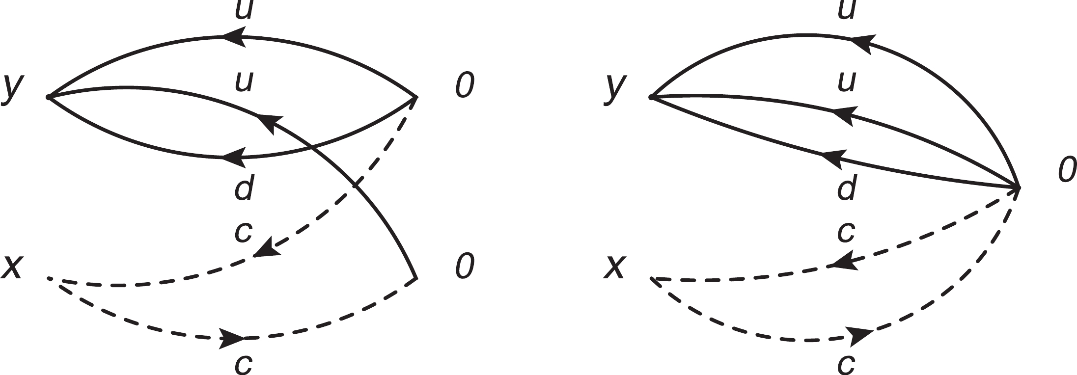
Figure 5. Lowest order Feynman diagrams contributing to decays of the pentaquark molecular state. In the first diagram, we take into account the finite spatial separation between the baryon and meson clusters.
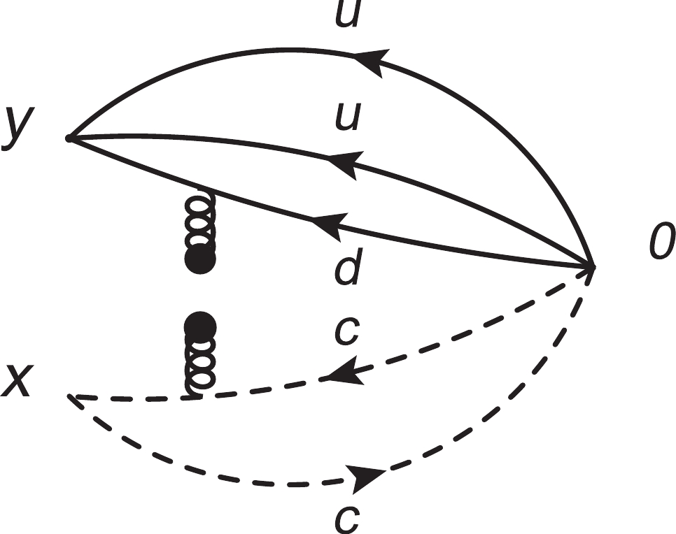
Figure 6. Non-factorizable Feynman diagrams contributing to the gluon condensate. Other diagrams obtained by interchanging of the light quark lines or heavy quark lines are implied.
$\begin{split} \Pi ({p^{\prime 2}},{p^2},{p^2}) =& \int_{4m_c^2}^\infty {\rm d} s\int_0^\infty {\rm d} u\dfrac{{{\rho _{\rm QCD}}(s,u)}}{{(s - {p^2})(u - {q^2})}} \\ &+{\rm{nonsingular}}\;{\rm{terms}}\;{\rm{of}}\;{p^{\prime 2}}, \end{split}$

(37) at the QCD side; there are both factorizable and non-factorizable contributions.
In previous section, we have proved that the current operator
$ J(x) $ couples potentially to the$ \Sigma_c\bar{D} $ molecular state, which receives both factorizable and non-factorizable contributions, while the couplings to the baryon-meson scattering states can be neglected. From Eqs. (15)-(18), we can see that there is a pole term$ \dfrac{1}{m_P^2-p^{\prime2}} $ at the hadron side, which should have originated at the QCD side. However, at the QCD side, there is no singular term with respect to the variable$ p^{\prime2} $ ; see Eq. (21). It does not imply that there is no contribution from$ P_c(4312) $ or that the current-molecule coupling$ \lambda_P $ is zero, it just means that$ P_c(4312) $ may not be on the mass-shell. If we set$ p^{\prime2} = p^2 $ to obtain the QCD sum rules, the terms$ \dfrac{1}{m_P^2-p^{2}} $ and$ \dfrac{1}{m_{J/\psi}^2-p^{2}} $ at the hadron side cannot be singular simultaneously. A reasonable explanation is that the current operator$ J(0) $ in the three-point correlation functions$ \Pi_5(p,q) $ and$ \Pi_{\mu}(p,q) $ couples potentially to the$ \Sigma_c\bar{D} $ molecular state or$ P_c(4312) $ . However, the$ P_c(4312) $ may not be on the mass-shell, which facilitates setting$ p^{\prime2} = p^2 $ . -
At the hadron side, we take the hadronic parameters as
$ m_{J/\psi} \!=\! 3.0969\;\rm{GeV} $ ,$ m_{N} \!=\! 0.93827\;\rm{GeV} $ ,$ m_{\eta_c} \!=\! 2.9839\;\rm{GeV} $ ,$ \sqrt{s^0_{J/\psi}}\! =\! 3.6\;\rm{GeV} $ ,$ \sqrt{s^0_{\eta_c}} \!=\! 3.5\;\rm{GeV} $ ,$ \sqrt{s^0_{N}} \!=\! 1.3\;\rm{GeV} $ [42],$ m_{P} \!=\! 4.3119\;\rm{GeV} $ [2],$ f_{J/\psi} = 0.418 \;\rm{GeV} $ ,$ f_{\eta_c} = 0.387 \;\rm{GeV} $ [43],$ \lambda_N = 0.032\;\rm{GeV}^3 $ [44], and$ \lambda_P = 1.95\times 10^{-3}\;\rm{GeV}^6 $ [18].At the QCD side, we take the standard values of the vacuum condensates
$ \langle \bar{q}q \rangle\! =\! -(0.24\!\pm\! 0.01\, \rm{GeV})^3 $ ,$ \langle \bar{q}g_s\sigma G q \rangle \!=\! m_0^2\langle \bar{q}q \rangle $ ,$ m_0^2 = (0.8 \pm 0.1)\,\rm{GeV}^2 $ , and$ \langle \dfrac{\alpha_s GG}{\pi}\rangle = (0.33\,\rm{GeV})^4 $ at the energy scale$ \mu = 1\, \rm{GeV} $ [35, 40, 41, 45], and choose the$ \overline{MS} $ mass$ m_{c}(m_c) = (1.275\pm0.025)\,\rm{GeV} $ from the Particle Data Group [42]. Moreover, we take into account the energy-scale dependence of the parameters,$ \begin{split} &\langle\bar{q}q \rangle(\mu) = \langle\bar{q}q \rangle(1\;{\rm{GeV}})\left[\dfrac{\alpha_{s}(1\;{\rm{GeV}})}{\alpha_{s}(\mu)}\right]^{\frac{12}{25}}\, , \\ &\langle\bar{q}g_s \sigma Gq \rangle(\mu) = \langle\bar{q}g_s \sigma Gq \rangle(1\;{\rm{GeV}})\left[\dfrac{\alpha_{s}(1\;{\rm{GeV}})}{\alpha_{s}(\mu)}\right]^{\frac{2}{25}}\, , \\& m_c(\mu) =m_c(m_c)\left[\dfrac{\alpha_{s}(\mu)}{\alpha_{s}(m_c)}\right]^{\frac{12}{25}} \, ,\\& \alpha_s(\mu) = \dfrac{1}{b_0t}\left[1-\dfrac{b_1}{b_0^2}\dfrac{\log t}{t} +\dfrac{b_1^2(\log^2{t}-\log{t}-1)+b_0b_2}{b_0^4t^2}\right]\, , \end{split} $

(38) where
$ t = \log \dfrac{\mu^2}{\Lambda^2} $ ;$ b_0 = \dfrac{33-2n_f}{12\pi} $ ;$ b_1 = \dfrac{153-19n_f}{24\pi^2} $ ;$ b_2 = \dfrac{2857-\dfrac{5033}{9}n_f+\dfrac{325}{27}n_f^2}{128\pi^3} $ ; and$ \Lambda = 210 $ ,$ 292$ ,$ 332\;\rm{MeV} $ for the flavors$ n_f = 5 $ ,$ 4 $ , and$ 3 $ , respectively [42, 46], and evolve all the parameters to the ideal energy scale$ \mu $ with$ n_f = 4 $ to extract the hadronic coupling constants$ g_5 $ ,$ g_V $ , and$ g_T $ .In the QCD sum rules for the mass of the
$ \bar{D}\Sigma_c $ pentaquark molecular state with the spin-parity$ J^P = {\dfrac{1}{2}}^- $ or$ P_c(4312) $ , the ideal energy scale of the QCD spectral density is$ \mu = 2.2\;\rm{GeV} $ [18], which is determined by the energy scale formula$ \mu = \sqrt{M^2_{X/Y/Z/P}-(2{\mathbb{M}}_c)^2} $ with the effective c-quark mass$ {\mathbb{M}}_c = 1.85\;\rm{GeV} $ [47]. The energy scale$ \mu = 2.2\;\rm{GeV} $ is too large for N,$ \eta_c $ , and$ J/\psi $ . In this study, we take the energy scales of the QCD spectral densities to be$ \mu = \dfrac{m_{\eta_c}}{2} = 1.5\;\rm{GeV} $ , which is acceptable for the charmonium states [37].We choose the values of the free parameters as
$ C_{5} = 1.18\times 10^{-6}\;\rm{GeV}^9 $ ,$ \overline{C}_{5} = 1.94\times 10^{-5}\;\rm{GeV}^{10} $ ,$ C_{V} = -1.77\times 10^{-5}\;\rm{GeV}^9 $ , and$ C_{T} = -1.67\times 10^{-5}\;\rm{GeV}^{9} $ to obtain flat platforms in the Borel windows$ T^2 = (3.1-4.1)\;\rm{GeV^2} $ ,$ (3.3-4.3)\;\rm{GeV^2} $ ,$ (4.0-5.0)\;\rm{GeV^2} $ , and$ (3.9-4.9)\;\rm{GeV^2} $ for the hadronic coupling constants$ g_5 $ ,$ g_V $ , and$ g_T $ , respectively. We fit the free parameters$ C_5 $ ,$ \overline{C}_5 $ ,$ C_V $ , and$ C_T $ to obtain the same intervals of flat platforms$ T_{\rm max}^2-T^2_{\rm min} = 1.0\;\rm{GeV}^2 $ , where$ T^2_{\rm max} $ and$ T^2_{\rm min} $ denote the maximum and minimum values of the Borel parameters, respectively.We take into account the uncertainties of the input parameters, and obtain the values of the hadronic coupling constants
$ g_5 $ ,$ g_V $ , and$ g_T $ , which are shown in Fig. 7,
Figure 7. (color online) Hadronic coupling constants
$ g_5 $ ,$ g_V $ , and$ g_T $ with variations of the Borel parameters$ T^2 $ , the values of$ g_5 $ in the first diagram and second diagram come from the QCD sum rules in Eq. (28) and Eq. (29), respectively.$ \begin{split} g_5& = 0.09\pm0.03\,\,\,\,{\rm{from}} \,\,\,\,{\rm{Eq.\;}}(28)\, ,\\ g_5& = 0.09\pm0.07\,\,\,\,{\rm{from}}\,\,\,\,{\rm{Eq.\;}}(29)\, ,\\ g_V& = 0.40\pm0.50\, ,\\ g_T& = 0.10\pm0.40\, , \end{split} $

(39) where we have redefined the hadronic coupling constants
$ g_V/g_T $ in Eq. (13) with a simple replacement,$ g_V/g_T \to -g_V/g_T $ , as the central values of$ g_V/g_T $ are negative from the QCD sum rules in Eq. (30).Now it is straightforward to calculate the partial decay widths of the decays
$ P_c(4312)\to \eta_c N $ ,$ J/\psi N $ ,$ \begin{split} \Gamma\left(P_c(4312)\to \eta_c N\right)& = \dfrac{p(m_P,m_{\eta_c},m_N)}{16\pi m_P^2} |T|^2\\ & = 31.488 g_5^2 \,\,{\rm{MeV}}\\ & = 0.255^{+0.198}_{-0.142}\;{\rm{MeV}}\,\,\,\,{\rm{from}} \,\,\,\,{\rm{Eq.\;}}(28)\, ,\\ & = 0.255^{+0.551}_{-0.242}\;{\rm{MeV}}\,\,\,\,{\rm{from}}\,\,\,\,{\rm{Eq.\;}}(29)\, , \end{split} $

(40) where
$ T = \bar{u}(q){\rm i} g_5 u(p^\prime)\, , $

(41) and
$ p(a,b,c) = \dfrac{\sqrt{[a^2-(b+c)^2][a^2-(b-c)^2]}}{2a} $ ,$ \begin{split} &\Gamma\left(P_c(4312)\to J/\psi N\right) = \dfrac{p(m_P,m_{J/\psi},m_N)}{16\pi m_P^2} |T|^2\\ & = 29.699 g_T^2 - 97.554g_V g_T + 80.633g_V^2\,\,{\rm{MeV}}\\ & = 9.296^{+19.542}_{-9.296}\,\,{\rm{MeV}}\, , \end{split} $

(42) where
$ \begin{align} T& = \varepsilon_\alpha^*\bar{u}(q)\left( g_V\gamma^\alpha-{\rm i}\dfrac{g_T}{m_P+m_N}\sigma^{\alpha\beta}p_\beta\right)\gamma_5 u(p^\prime)\, . \end{align} $

(43) The partial decay width
$ \Gamma\left(P_c(4312)\to \eta_c N\right) = 0.255 $ MeV is extremely small, and the total width$ \Gamma_{P_c(4312)} $ can be saturated with the strong decay$ P_c(4312)\to J/\psi N $ . The predicted width$ \Gamma\left(P_c(4312)\to J/\psi N\right) = 9.296^{+19.542}_{-9.296} $ MeV is compatible with the experimental data$ \Gamma_{P_c(4312)} = 9.8\pm2.7^{+ 3.7}_{- 4.5} \;{\rm{ MeV}} $ from the LHCb collaboration [2]. The present calculations support assigning$ P_c(4312) $ to be the$ \bar{D}\Sigma_c $ pentaquark molecular state with the spin-parity$ J^P = {\dfrac{1}{2}}^- $ . We can search for$ P_c(4312) $ in the$ \eta_cN $ mass spectrum, and measure the branching fraction$ {\rm Br}\left(P_c(4312)\to \eta_c N\right) $ , which may shed light on the nature of$ P_c(4312) $ and test the predictions of the QCD sum rules.The thresholds of
$ \bar{D}\Lambda_c $ and$ \bar{D}^*\Lambda_c $ are$ 4.15\;\rm{GeV} $ and$ 4.29\;\rm{GeV} $ , respectively, and the decays into the final states$ \bar{D}\Lambda_c $ and$ \bar{D}^*\Lambda_c $ are kinematically allowed. At the quark level, the decays of the$ \bar{D}\Sigma_c $ pentaquark molecular state to the$ \bar{D}\Lambda_c $ and$ \bar{D}^*\Lambda_c $ states take place through dissolving of the$ \Sigma $ -type diquark states to form the$ \Lambda $ -type diquark states by emitting an isospin$ I = 1 $ quark-antiquark pair. At the hadron level, the decay$ P_c(4312)\to\bar{D}^*\Lambda_c $ can take place through the process$ P_c(4312)\to\bar{D}\Sigma_c \to\bar{D}\Lambda_c\pi \to \bar{D}^*\Lambda_c $ with the subprocesses$ \Sigma_c\to \pi\Lambda_c $ and$ \bar{D}\pi\to\bar{D}^* $ ; the partial decay width$ \Gamma(P_c(4312)\to \bar{D}^*\Lambda_c) $ may be as large as$ 10.7\;\rm{MeV} $ [48]. Direct calculations of these partial decay widths with the QCD sum rules are necessary to make a definite conclusion, which we aim to address in our next work. -
In this article, we tentatively assign
$ P_c(4312) $ to be the$ \bar{D}\Sigma_c $ pentaquark molecular state with the spin-parity$ J^P = {\dfrac{1}{2}}^- $ , and discuss the factorizable and non-factorizable contributions in the two-point QCD sum rules for the$ \bar{D}\Sigma_c $ molecular state in detail to prove the reliability of the single pole approximation in the hadronic spectral density. We study its two-body strong decays with the QCD sum rules by carrying out the operator product expansion up to the vacuum condensates of dimension$ 10 $ . In calculations, special attention was paid to match the hadron side with the QCD side of the correlation functions to obtain solid duality. We obtain the partial decay widths$ \Gamma\left(P_c(4312)\to \eta_c p\right) = 0.255\;{\rm{MeV}} $ and$ \Gamma\left(P_c(4312)\to J/\psi p\right) = 9.296^{+19.542}_{-9.296}\,\,{\rm{MeV}} $ , which are compatible with the experimental data$ \Gamma_{P_c(4312)} = 9.8\pm2.7^{+ 3.7}_{- 4.5} \;{\rm{ MeV}} $ from the LHCb collaboration. The present calculations support assigning$ P_c(4312) $ to be the$ \bar{D}\Sigma_c $ pentaquark molecular state with the spin-parity$ J^P = {\dfrac{1}{2}}^- $ . We can search for the decay$ P_c(4312)\to \eta_c p $ to diagnose the nature of$ P_c(4312) $ .
Analysis of the strong decays of Pc(4312) as a pentaquark molecular state with QCD sum rules
- Received Date: 2020-05-25
- Available Online: 2020-10-01
Abstract: In this article, we tentatively assign


 DownLoad: