


 Abstract
 HTML
HTML Reference
 Related
 PDF
PDF


-
Accretion around a massive gravitational object is a basic phenomenon in astrophysics and has been essential to the understanding of various astrophysical processes and observations, including the growth of stars, the formation of supermassive black holes, quasar luminosity, and X-ray emission from compact star binaries [1-3]. The accretion of matter in a realistic astrophysical process is rather complicated, since it involves many challenging aspects of general relativistic magnetohydrodynamics, including turbulence, radiation processes, and nuclear burning. To understand these accretion processes, it is useful to simplify the problem by making assumptions and/or considering simple scenarios.
The simplest accretion scenario describes a stationary, spherically symmetric solution, as first discussed by Bondi [4], where an infinitely large homogeneous gas cloud, steadily accreting onto a central gravitational object, was considered. Bondi's treatment was formulated in the framework of Newtonian gravity. Later, in the framework of general relativity (GR), the steady-state spherically symmetric flow of a test fluid onto a Schwarzschild black hole was investigated by Michel [5]. Since then, spherical accretion has been considered for various spherically symmetric black holes in GR and modified gravities; see [6-30] and references therein for examples.
One important feature of spherical accretion onto black holes is the phenomenon of transonic accretion and the existence of a sonic point (or a critical point). At the sonic point, the accretion flow transits from the subsonic to the supersonic state. Normally, the locations of the sonic points in a given black hole spacetime are not far from its horizon. What is important and intriguing is that the narrow region around the sonic point is closely related to some ongoing observations about the spectra of electromagnetic and gravitational waves. Therefore, studying the spherical accretion problem can not only help us to understand accretion processes in different black holes but, importantly, also provide us with an alternative approach to explore the nature of the black hole spacetimes in the regime of strong gravity.
On the other hand, the EHT collaboration recently reported their first image concerning the detection of the shadow of a supermassive black hole at the center of a neighboring elliptical M87 galaxy [31-36]. This image revealed that the diameter of the center black hole shadow is
$ (42\pm 3) \;$ μ, leading to the measured center mass$ M = (6.5\pm 0.7)\times 10^9 M_{\odot} $ [31]. The outer edge of the shadow image, if one considers a Schwarschild black hole, forms a photon sphere near the black hole horizon, at which the trajectories of photons create a closed circular orbit. Within astrophysical observations, the existence of a photon sphere is related to the electromagnetic observations of black holes via the background electromagnetic emission and the frequencies of quasi-normal modes. The latter is determined by the parameters of null geodesic motions on and near the photon sphere of a given black hole spacetime.Recently, it was shown that there is a correspondence between the sonic points of an accreting ideal photon gas and the photon sphere, for static spherically symmetric spacetimes [37]. This important result is valid not only for spherical accretion of the ideal photon gas but also for rotating accretion in static spherically symmetric spacetimes [38, 39]. In an observational viewpoint, as mentioned in [39], this correspondence connects two independent observations, the observation of light coming from sources behind a black hole and the observation of emission from the accreted radiation fluid onto the black hole. This is because the size of the hole's shadow is determined by the radius of the photon sphere, and the accreted fluid can signal the sonic point.
In light of the above studies, it is interesting to explore spherical accretion flows in different black hole spacetimes. The additional parameters, beyond the Schwarzschild black hole in these spacetimes, may affect the accretion flow behavior; thus, we have a potentially important approach for studying the strong gravity behavior of black holes in many alternative theories of gravity. Instead of finding the exact solution and studying the spherical accretion case by case for each given theory, a reasonable strategy is to consider a model-independent framework that parameterizes the most generic black-hole geometry through a finite number of adjustable quantities. For this purpose, in this paper, we consider spherical accretion flows in general parameterized spherically symmetric black hole spacetimes [40]. This parameterized description allows one to consider accretion phenomena not only for specific theories of gravity but also for analysis in a unified way by exploring the influence of different black hole parameters on the spherical accretion process [40]. Specifically, we focus our attention on the perfect fluid accretion onto general parameterized spherically symmetric black hole spacetimes and further investigate transonic phenomena for different fluids, including isothermal fluids and polytropic fluids. By studying the accretion of the ideal photon gas, we further reveal the correspondence between the sonic points of the accreting photon gas and the photon sphere, for general parameterized spherically symmetric black holes.
Our paper is organized as follows. In Sec. 2, we present a very brief introduction to general parameterized spherically symmetric black holes. Then, in Sec. 3, we derive the basic equations for subsequent discussions on the spherical accretion of various fluids and present several useful quantities. Sec. 4 is devoted to performing a dynamical systems analysis of the accretion process and finding the critical points of the system. In Sec. 5, we apply these results to several known fluids and further investigate the transonic phenomena of the accretion of these fluids onto general parameterized spherically symmetric black holes. In Sec. 6, by studying the spherical accretion of the ideal photon gas and photon sphere of general parameterized spherically symmetric black holes, we establish the correspondence between the sonic points of the ideal photon gas and its photon sphere. The conclusion of this paper is presented in Sec. 7.
-
In this section, we present a brief introduction to the parameterization by L. Rezzolla and A. Zhidenko's (RZ) [40], for generic spherically symmetric black hole spacetimes. First, let us consider the line element of any spherically symmetric stationary configuration in the spherical polar coordinate system
$ (t, r, \theta, \phi) $ , which can be written as$ {\rm d}s^2 = - N^2(r) {\rm d}t^2 + \frac{B^2(r)}{N^2(r)}{\rm d}r^2 + r^2 ({\rm d}\theta^2 + \sin^2\theta {\rm d}\phi^2), $

(1) where
$ N(r) $ and$ B(r) $ are two functions of the radial coordinate r alone. In the RZ parameterization,$ N(r) $ is expressed as$ N^2(x) = x A(x), $

(2) where
$ A(x) >0 $ for$ 0<x<1 $ with$ x = 1- r_0/r $ . It is obvious that$ x = 0 $ represents the location of the event horizon of the black hole, and$ x = 1 $ is the spatial infinity. Then, the functions$ A(x) $ and$ B(x) $ can be further parameterized in terms of the parameters$ \epsilon $ ,$ a_i $ , and$ b_i $ as$ A(x) = 1 - \epsilon(1-x) +(a_0-\epsilon)(1-x)^2+ \tilde{A}(x) (1-x)^3, $

(3) $ B(x) = 1 + b_0 (1-x) + \tilde{B}(x) (1-x)^2, $

(4) where the functions
$ \tilde{A} $ and$ \tilde{B} $ are introduced to describe the metric near the horizon (i.e.,$ x \simeq 0 $ ) and at the spatial infinity (i.e.,$ x = 1 $ ). The coefficients$ a_0 $ and$ b_0 $ can be seen as combinations of the PPN parameters. The functions$ \tilde A $ and$ \tilde B $ can be expanded using the continuous Padé approximation as$ \tilde A(x) = \frac{a_1}{1+ \dfrac{a_2 x}{1+ \frac{a_3 x}{1+ \cdots }}},\;\;\;\;\; \tilde B(x) = \frac{b_1}{1+ \dfrac{b_2 x}{1+ \frac{b_3 x}{1+ \cdots }}}, $

(5) where
$ a_1, a_2, \cdots, a_n $ and$ b_1, b_2, \cdots, b_n $ are dimensionless constants that can be determined by matching the above parameterization to a specific metric. In addition, the parameter$ \epsilon $ in the RZ parameterization measures the deviation of the position of the event horizon in the general metric from the corresponding location in the Schwarzschild spacetime, i.e.,$ \epsilon = \frac{2 M - r_0}{r_0}. $

(6) The RZ parameterization can be matched to many black hole solutions which differ from GR. These include the Reissner-Nordström (RN) black hole in GR and black holes in the Brans-Dicke gravity (BD),
$ f(R) $ gravity, the Einstein-Maxwell axion dilaton theory (EMAD), and the Einstein-Aether theory [40, 41]. Recently, the RZ parameterization has also been extended to the rotating case [42]. -
In this section, we consider the steady-state spherical accretion flow of matter near an RZ-parameterized black hole. For this purpose, the accreting matter is approximated as a relativistic perfect fluid, by neglecting effects related to viscosity or heat transport. Thus, the energy momentum tensor of the fluid can be described by
$ T^{\mu \nu} = (\rho+p)u^\mu u^\nu + p g^{\mu\nu}, $

(7) where
$ \rho $ and p are the proper energy density and the pressure of the perfect fluid. The four-velocity$ u^\mu $ obeys the normalization condition$ u_\mu u^\mu = -1 $ . We assume that the fluid is radially flowing into the black hole; therefore, we have$ u^\theta = 0 = u^\phi $ . For the same reason, the physical quantities ($ \rho $ , p) and others introduced later are functions of the radial coordinate r only. For the sake of simplicity, we set the radial velocity as$ u^r = u <0 $ for the accreting case. Then, using the normalization condition, it is easy to infer that$ (u^t)^2 = \frac{N^2(r)+B^2(r) u^2}{N^4(r)}. $

(8) There are two basic conservation laws that govern the evolution of a fluid in a black hole spacetime. One is the conservation law of the particle number, and another one is the conservation law of the energy momentum. The assumption of the conservation of the particle number implies there is no particle creation and/or annihilation during the accreting process. Defining the proper particle number density n and number current
$ J^\mu = n u^\mu $ in the local inertial rest frame of the fluid, the conservation of the particle number gives$ \nabla_\mu J^\mu = \nabla_{\mu} (n u^\mu) = 0, $

(9) where
$ \nabla_\mu $ denotes the covariant derivative with respect to the coordinate. For the RZ parameterization of a generic spherically symmetric black hole spacetime, Eq. (9) can be rewritten as$ \frac{1}{r^2 B} \frac{\rm d}{{\rm d} r}(r^2 B n u) = 0. $

(10) Integrating this equation, we obtain
$ r^2 B n u = C_1, $

(11) where
$ C_1 $ is the integration constant.The conservation law of the energy momentum is expressed as
$ \nabla_\mu T^{\mu \nu} = 0. $

(12) It is also convenient to introduce the first law of the thermodynamics of the perfect fluid, which is given by [43]
$ {\rm d}p = n ({\rm d}h - T {\rm d}s),\; \; \; {\rm d}\rho = h {\rm d}n +nT {\rm d}s, $

(13) where T is the temperature, s is the specific entropy, and h is the specific enthalpy, defined as
$ h \equiv \frac{\rho + p}{n}. $

(14) Then, projecting the conservation law of the energy-momentum (12) along
$ u^\mu $ , one obtains$ \begin{aligned}[b] u_{\nu}\nabla_{\mu} T^{\mu\nu} & = u_{\nu} \nabla_{\mu} \Big[ nh u^{\mu} u^{\nu} + p g^{\mu\nu}\Big] \\ & = - n u^{\mu} \nabla_{\mu} h + u^{\mu} \nabla_{\mu} p. \end{aligned} $

(15) In the above, we have used the conservation of the particle number, i.e.,
$ \nabla_{\mu} (n u^{\mu}) = 0 $ and$ u^{\mu} \nabla_{\nu} u_{\mu} = u_{\mu} \nabla_{\nu} u^{\mu} =$ $ \frac{1}{2} \nabla_{\nu} (u^{\mu}u_{\mu}) = 0 $ . Noticing that the first law of thermodynamics (13) can be rewritten as$ \nabla_{\mu }p = n \nabla_{\mu} h - n T \nabla_{\mu}s $ , from the above projection one arrives at$ - n T u^{\mu} \nabla_{\mu} s = 0, $

(16) implying that there is no heat transfer between the different fluid elements, and the specific entropy is conserved along the evolution lines of the fluid. For a parameterized spherically symmetric black hole, the conservation of the specific entropy reduces to
$ \partial_r s = 0 $ , i.e.,$ s = $ constant. For this reason, the fluid is isentropic and Eq. (13) reduces to$ {\rm d}p = n {\rm d}h,\; \; \; \; {\rm d}\rho = h {\rm d}n. $

(17) With the above thermodynamical properties of the perfect fluid, the conservation law of the energy-momentum (12) can be written as
$ \begin{aligned}[b] \nabla_\mu T^{\mu}_{\nu} & = \nabla_{\mu} (h n u^\mu u_\nu) +\nabla_{\mu} (\delta^\mu_\nu p) \\ & = n u^{\mu} \nabla_{\mu} (h u_\nu) + n \nabla_{\nu }h \\ & = n u^{\mu} \partial_{\mu} (h u_\nu) - n u^{\mu} \Gamma_{\mu \nu}^\lambda h u_{\lambda}+ n \nabla_{\nu }h = 0. \end{aligned} $

(18) Then, the time component
$ \nu = t $ of the above equation yields$ \partial _r(hu_t) = 0. $

(19) Integrating it for the parameterized spherically symmetric black hole we consider in this paper, one arrives at
$ h \sqrt{N^2 +B^2u^2} = C_2, $

(20) where
$ C_2 $ is the integration constant. This equation, together with Eq. (11), constitutes the two basic equations describing a radial, steady-state perfect fluid flow in the parameterized spherically symmetric black hole.To proceed further, let us introduce several useful quantities for describing the accretion flow, which will be used in the subsequent analysis. The first quantity is the sound speed of the perfect fluid, which is defined by
$ c_s^2 \equiv \frac{{\rm d} p}{{\rm d} \rho} = \frac{n}{h}\frac{{\rm d} h}{{\rm d} n} = \frac{{\rm d} \ln h }{{\rm d} \ln n}. $

(21) On the other hand, by considering radial accretion flows, i.e.,
$ {\rm d} \theta = {\rm d} \phi = 0 $ , the black hole metric can be decomposed as [44]$ {\rm d}s^2 = - (N {\rm d}t)^2 + \left(\frac{B}{N}{\rm d}r \right)^2, $

(22) from which one can define an ordinary three-dimensional velocity v measured by a static observer as
$ v \equiv \frac{B}{N^2} \frac{{\rm d}r}{{\rm d}t}. $

(23) Considering
$ u^{r} = u = {\rm d}r/{\rm d}\tau $ and$ u^t = {\rm d}t /{\rm d}\tau $ with$ \tau $ being the proper time of the fluid, one finds$ v^2 = \frac{B^2}{N^4} \left(\frac{u}{u^t}\right)^2 = \frac{B^2 u^2}{N^2+B^2 u^2}. $

(24) Then, one can express
$ u^2 $ and$ u_t^2 $ in terms of$ v^2 $ as$ u^2 = \frac{N^2 v^2}{B^2(1-v^2)}, $

(25) $ u^2_t = \frac{N^2}{1-v^2}. $

(26) These quantities will be used in the following dynamical systems analysis for the radial, steady-state perfect fluid flow in a parametrized spherically symmetric black hole.
-
The two basic equations (11) and (20) constitute a dynamical system for the radial accretion process. In this section, we use these equations to study the accretion process in a parametrized spherically symmetric black hole.
-
In the trajectories of an accretion flow into a black hole, there exists a specific point called the sonic point, at which the four-velocity of the moving fluid becomes equal to the local speed of sound, and the accretion flow attains the maximal accretion rate. To determine the sonic point, let us first take the derivative of the two basic equations (11) and (20) with respect to r, which leads to
$ \left(v^2 - c_s^2\right) \frac{{\rm d} \ln v}{{\rm d}r} = \frac{1-v^2}{B N r} \left[ c_s^2 N B \left(2 +r \frac{{\rm d}\ln B}{{\rm d}r}\right)- B (1-c_s^2) r \frac{{\rm d}N}{{\rm d}r}\right]. $

(27) At the sonic point
$ r_* $ ($ c_s^2(r_*) = v^2(r_*) $ ), one has$ c_{s*}^2 N_* B_* \left(2 +r_* \left.\frac{{\rm d}\ln B}{{\rm d}r}\right|_*\right)- B_* (1-c_{s*}^2) r_* \left.\frac{{\rm d}N}{{\rm d}r}\right|_* = 0, $

(28) where
$ * $ denotes the values evaluated at the sonic point. This equation allows us to determine the sonic point once the speed of sound$ c_s^2 \equiv {\rm d}p/{\rm d}\rho $ is known. The above equation can be rewritten as$ u_*^2 = \frac{N_* r_*\left.\dfrac{{\rm d}N}{{\rm d}r}\right|_*}{B_*^2 \left(2 +r_* \left.\dfrac{{\rm d}\ln B}{{\rm d}r}\right|_*\right)}. $

(29) Therefore, once
$ r_* $ is determined, one can use this expression to find the value of u at the sonic point. The existence of the sonic point in the black hole spacetime physically exhibits a very interesting accreting phenomenon; it highlights transonic solutions that are supersonic near and subsonic far from the black hole. In the following sections, we are going to find sonic points by using the equations obtained in this subsection and discuss the transonic phenomenon in detail for different fluids. -
From the two basic equations (11) and (20), we observe that there are two integration constants
$ C_1 $ and$ C_2 $ . For this system, we may treat the square of the left-hand side of Eq. (20) as a Hamiltonian$ {\cal H} $ of this system,$ {\cal H} = h^2 (N^2+B^2 u^2), $

(30) so
$ C_2 $ of every orbit in the phase space of this system is kept fixed. Inserting Eq. (25) into the Hamiltonian$ {\cal H} $ one finds$ {\cal H}(r,v) = \frac{h^2(r,v)N^2}{1-v^2}. $

(31) Then, the dynamical system associated with this Hamiltonian reads
$ \dot{r} = {\cal H}_{,v} ,\; \; \; \; \dot{v} = -{\cal H}_{,r}, $

(32) where the dot denotes the derivative with respect to
$ \bar t $ (the time variable of the Hamiltonian dynamical system). Then, inserting the Hamiltonian, one finds$ \dot{r} \equiv f(r,v) = \frac{2 h^2 N^2}{v(1-v^2)^2} (v^2 - c_s^2), $

(33) $ \dot{v} \equiv g(r,v) = -\frac{h^2 }{r (1-v^2)} \left[r N^2_{,r} (1 - c_s^2) - 4 N^2 c_s^2\right]. $

(34) These equations constitute an autonomous, Hamiltonian two-dimensional dynamical system. Its orbits are composed of the solutions of the two basic Eqs. (11) and (20). In the construction of the above dynamical system, we considered the two quantities
$ (r, v) $ as the two dynamical variables of the system. It is worth mentioning that there are actually different ways to select dynamical variables; for example, one may choose the dynamical variables to be$ (r, h) $ ,$ (r, p) $ , or$ (r, u) $ [45].At critical points, the right-hand sides of Eqs. (33) and (34) vanish, and the following equations provide a set of critical points that are solutions to
$ \dot{r} = 0 $ and$ \dot{v} = 0 $ ,$ v_*^2 = c_s^2, $

(35) $ c_s^2 = \frac{r_* N^2_{*,r_*}}{r_* N^2_{*,r_*} + 4N^2_{*,r_*}} . $

(36) It is easy to see that sonic points are the critical points of this dynamical system. Hereafter, we use
$ (r_*, v_*) $ to denote the critical points of the dynamical system. For a dynamical system, critical points can be divided into several different types. To observe which critical points could arise from the black hole accretion processes, let us perform the following linearization of the dynamical system by Taylor-expanding Eqs. (33) and (34) around the critical points, i.e.,$ \left( \begin{array}{c} {\delta \dot r} \\ {\delta \dot v} \end{array}\right) = X \left( \begin{array}{c} \delta r \\ \delta v \end{array}\right), $

(37) where
$ \delta r $ ,$ \delta v $ denote the small perturbations of r, v about the critical points, and X is the Jacobian matrix of the dynamical system at the critical point$ (r_*, v_*) $ , which is defined as$ X = \left(\begin{array}{*{20}{c}} \dfrac{\partial{f}}{\partial{r}} & \dfrac{\partial{f}}{\partial{v}} \\ \dfrac{\partial{g}}{\partial{r}} & \dfrac{\partial{g}}{\partial{v}} \end{array}\right)\Bigg|_{(r_*, v_*)}. $

(38) Depending on the determinant
$ \Delta = {\rm{det}} (X) $ of X and its trace$ \chi = {\rm Tr}(X) $ , the types of the critical points$ (r_*, v_*) $ of the dynamcial system can be summarized as follows:● Saddle points if
$ \Delta <0 $ .● Attracting nodes if
$ \Delta >0 $ ,$ \chi < 0 $ , and$ \chi^2-4\Delta >0 $ .● Attracting spirals if
$ \Delta >0 $ ,$ \chi < 0 $ , and$ \chi^2-4\Delta <0 $ .● Repelling nodes if
$ \Delta >0 $ ,$ \chi > 0 $ , and$ \chi^2-4\Delta >0 $ .● Repelling spirals if
$ \Delta >0 $ ,$ \chi > 0 $ , and$ \chi^2-4\Delta <0 $ .● Degenerate nodes if
$ \Delta >0 $ , and$ \chi^2-4\Delta = 0 $ .● Centers if
$ \Delta >0 $ ,$ \chi = 0 $ .● Line or plane critical points if
$ \Delta = 0 $ .When the critical points and their types are determined, the constant
$ C_1 $ in Eq. (11) can be rewritten in terms of the quantities evaluated at the critical point$ (r_*, v_*) $ as$ C^2 _1 = \frac{r^4 _* n^2 _* v^2 _* N^2_*}{1 -v^2 _*} = \frac{r^5 _* n^2 _* N^2_{*,r_*}}{4}. $

(39) This equation is satisfied not only at the critical point but also at any point in the same streamline in the phase portrait, so one can easily get
$ \left(\frac{n}{n_*}\right)^2 = \frac{r^5_* N^2_{*,r_*}}{4}\frac{1- v^2}{r^4 N^2 v^2}. $

(40) If there is no solution to Eqs. (33) and (34) at the critical point, one can introduce any reference point
$ (r_0,v_0) $ from the phase portrait, obtaining [46]$ \left(\frac{n}{n_0}\right)^2 = \frac{r^4_0 N^2_0 v^2_0}{1- v^2_0}\frac{1- v^2}{r^4 N^2 v^2}. $

(41) The above expressions will be used later to analyze the spherical accretion processes for some test fluids.
-
In this section, we consider the accretion processes of several test fluids, using the equations derived in the above sections for a parameterized spherically symmetric black hole. Specifically, we consider the isothermal and polytropic fluids in the following subsections.
-
In this subsection, we consider the accretion processes for isothermal (constant-temperature) fluids. The corresponding system can be viewed as an adiabatic one, owing to the fast movement of the fluid. For such a system, we define its equation of state (EoS) w as
$ w\equiv p/\rho. $

(42) where
$ \rho $ and p represent the energy density and pressure of the fluid, respectively. It is worth noting that$ 0< w \leqslant 1 $ for isothermal fluids [20]. In addition, the adiabatic speed of sound is given by$ c_s^2 \equiv \dfrac{{\rm d} p}{{\rm d} \rho} = w $ .According to
$ h = (\rho+p)/n = (1+w)\rho/n $ and$c_s^2 = $ $ {\rm d}\ln h/ {\rm d}\ln n = w $ , we have$ \rho = \rho_0 \left(\frac{n}{n_0}\right)^{1+w}, $

(43) and
$ h = \frac{(w+1) \rho_0}{n_0} \left(\frac{n}{n_0} \right)^w, $

(44) where
$ n_0 $ and$ \rho_0 $ denote the values of n and$ \rho $ evaluated at some reference point. Using Eq. (40), we arrive at$ h^2 = K\left( \frac{1- v^2}{r^4 N^2 v^2}\right)^w, $

(45) where K is a constant. Through the transformation
$ \bar{t} \rightarrow K\bar{t} $ and$ {\cal H} \rightarrow {\cal H}/K $ , the constant K is absorbed into the redefined time$ {\bar{t}} $ . Then, the new Hamiltonian becomes$ {\cal H}(r,v) = \frac{N^{2(1-w)}}{(1-v^2)^{1-w} v^{2w} r^{4w}}. $

(46) Considering the first-order RZ parameterization (taking only the first three items of Eq. (3)), one can approximately write
$ N^2 \simeq \left(1-\frac{2M}{r(1+\epsilon)}\right)\left[1+\frac{4 M^2 (a_0- \epsilon)}{r^2 (1+\epsilon)^2} - \frac{2 M \epsilon }{r(1+\epsilon)}\right]. $

(47) Then, Eq. (46) can be approximately rewritten as
$\begin{aligned} {\cal H} \simeq \frac{\left(1-\dfrac{2M}{r(1+\epsilon)}\right)^{1-w} \left[1+\dfrac{4 M^2 (a_0- \epsilon)}{r^2 (1+\epsilon)^2} - \dfrac{2 M \epsilon }{r(1+\epsilon)}\right]^{1-w}}{(1-v^2)^{1-w} v^{2w} r^{4w}}. \end{aligned}$

(48) At the sonic point, with
$ c_s^2 = w $ , Eq. (34) reduces to$ w = \left. \frac{r N^2_{,r}}{r N^2_{,r} + 4 N^2} \right|_{r = r_*}. $

(49) With Eq. (47), Eq. (49) can be approximately rewritten as
$ w = \frac{M [-12 M^2 \epsilon + r_*^2 (1 + \epsilon)^3 + 4 a_0 M (3 M - r_* (1 + \epsilon))]}{LT_1}, $

(50) where
$\begin{aligned}[b] LT_1 =& 4 M^3 \epsilon - 3 M r_*^2 (1 + \epsilon)^3 + 2 r_*^3 (1 + \epsilon)^3 \\&+ 4 a_0 M^2 (-M + r_* + r _*\epsilon).\end{aligned} $

(51) -
Let us first consider an ultra-stiff fluid, whose energy density is equal to its pressure. In this case, the equation of state is
$ w = p/\rho = 1 $ . The Hamiltonian (48) for the ultra-stiff fluid becomes$ {\cal H} = \frac{1}{v^2 r^4}. $

(52) For physical flows, one has
$ |v| <1 $ . Therefore, the Hamiltonian (52) for the ultra-stiff fluid has a minimal value$ {\cal H}_{\rm min} = r_0^{-4} $ . With Eq. (52), the two-dimensional dynamical system (33), (34) is$ \dot{r} = - \frac{2}{r^4 v^3}, $

(53) $ \dot{v} = \frac{4}{r^5 v^2} . $

(54) It is easy to see that this dynamical system has no critical points. The phase space portrait of this dynamical system for the ultra-stiff fluid with
$ M = 1 $ ,$ a_0 = 0.001 $ , and$ \epsilon = 0.1 $ for a general parameterized black hole is depicted in Fig. 1, in which the physical flow of the ultra-stiff fluid in the general parameterized black hole is represented by several curves with arrows. It is shown that the curves with$ v<0 $ have arrows directed toward the black hole, representing the accreting flow of the ultra-stiff fluid, while the curves with$ v>0 $ have arrows directed toward the outside, representing the outflow fluids. The green and red curves represent the flows with minimal Hamiltonian$ {\cal H}_{\rm min} $ for the accretion outflow. All of the flows in Fig. 1 between the red and green curves are physical and have Hamiltonian$ {\cal H} > {\cal H}_{\rm min} $ .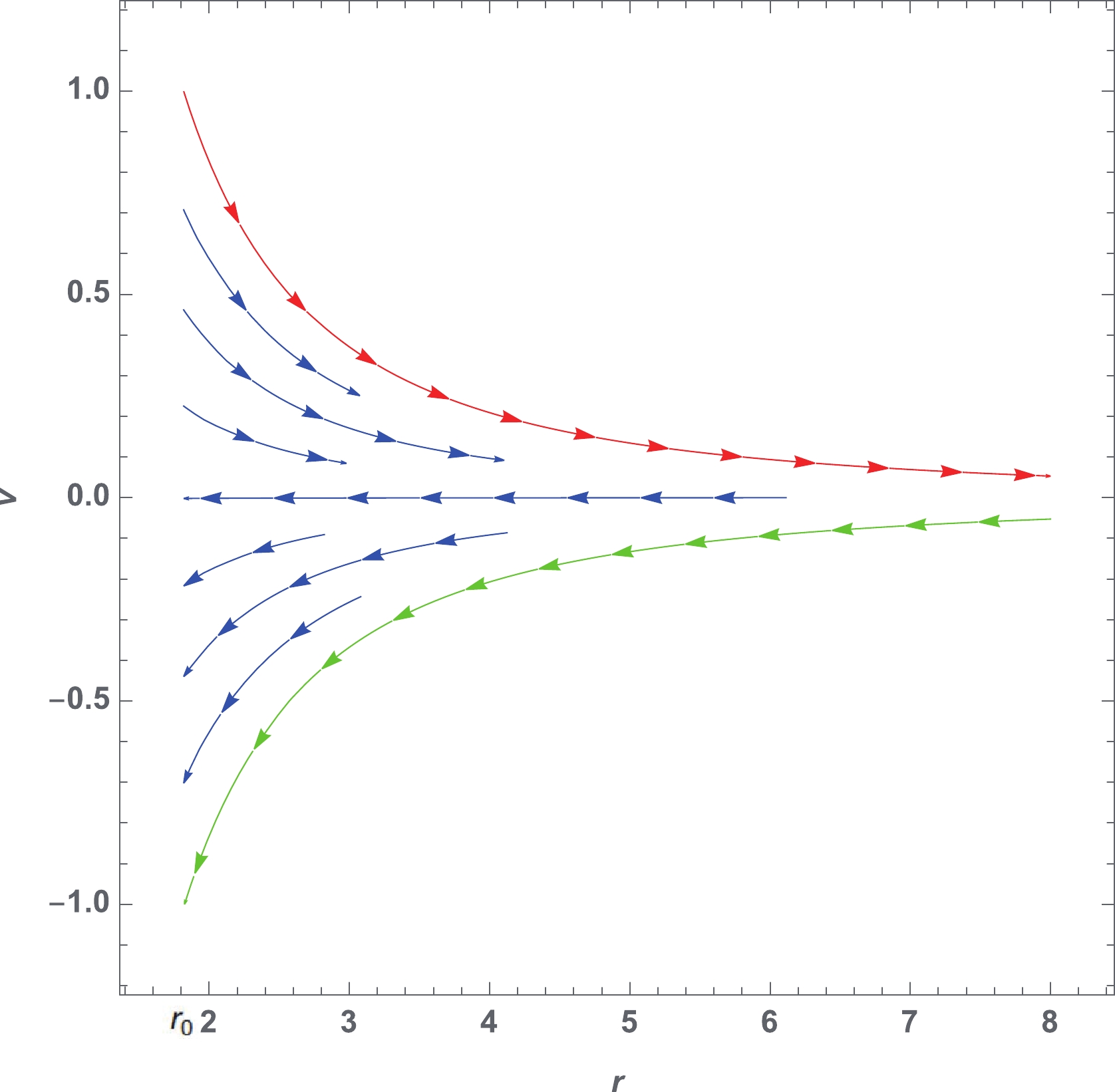
Figure 1. (color online) Phase space portrait of the dynamical system (33), (34) for the ultra-stiff fluid (
$ w = 1 $ ) with the black hole parameters$ M = 1 $ ,$ \epsilon = 0.1 $ , and$ a_0 = 0.0001 $ .The values of the minimal Hamiltonian
$ {\cal H}_{\rm min} $ depend on the RZ parameterization parameters. In Table 1, the values of$ r_0 $ and$ {\cal H} $ for the different values of parameter$ \epsilon $ for the ultra-stiff fluid are presented. Since the horizon radius decreases with respect to$ \epsilon $ , it is shown clearly that the minimal Hamiltonian$ {\cal H}_{\rm min} = 1/r_0^4 $ increases with increasing$ \epsilon $ .$ \epsilon $ 

$ 0 $ 

$ 0.1 $ 

$ 0.2 $ 

$ 0.3 $ 

$ 0.4 $ 

$ 0.5 $ 

$ r_0 $ 

$ 2 $ 

$ 1.81818 $ 

$ 1.66667 $ 

$ 1.53846 $ 

$ 1.42857 $ 

$ 1.33333 $ 

${\cal H}_{\rm min}$ 

$ 0.0625 $ 

$ 0.0915063 $ 

$ 0.1296 $ 

$ 0.178506 $ 

$ 0.2401 $ 

$ 0.316406 $ 

Table 1. Values of
$ r_0 $ and$ {\cal H}_{\rm min} $ for different values of the black hole parameter$ \epsilon $ for the ultra-stiff fluid with$ w=1 $ . In the calculation, we set$ M=1 $ and$ a_0=10^{-4} $ . -
Let us now consider an ultra-relativistic fluid, for which the equation of state is
$ w = 1/2 $ , i.e.,$ p = \rho/2 $ . In this case, the fluid's isotropic pressure is less than its energy density. With$ w = 1/2 $ , the Hamiltonian (48) becomes$ {\cal H} = \dfrac{\left(1-\dfrac{2M}{r(1+\epsilon)}\right)^{1/2} \left[1+\dfrac{4 M^2 (a_0- \epsilon)}{r^2 (1+\epsilon)^2} - \dfrac{2 M \epsilon }{r(1+\epsilon)}\right]^{1/2}}{ r^{2}|v|(1-v^2)^{1/2} }, $

(55) and then, the two-dimensional dynamical system (33), (34) is
$ \begin{aligned}[b] \dot{r} = &\frac{\left(1-\dfrac{2M}{r(1+\epsilon)}\right)^{1/2} \left[1+\dfrac{4 M^2 (a_0- \epsilon)}{r^2 (1+\epsilon)^2} - \dfrac{2 M \epsilon }{r(1+\epsilon)}\right]^{1/2}}{ r^{2}(1-v^2)^{3/2} } \\ &-\frac{\left(1-\dfrac{2M}{r(1+\epsilon)}\right)^{1/2} \left[1+\dfrac{4 M^2 (a_0- \epsilon)}{r^2 (1+\epsilon)^2} - \dfrac{2 M \epsilon }{r(1+\epsilon)}\right]^{1/2}}{ r^{2}v^2(1-v^2)^{1/2} }, \end{aligned}$

(56) $ \begin{aligned}[b] \dot{v} = &\frac{2\left(1-\dfrac{2M}{r(1+\epsilon)}\right)^{1/2} \left[1+\dfrac{4 M^2 (a_0- \epsilon)}{r^2 (1+\epsilon)^2} - \dfrac{2 M \epsilon }{r(1+\epsilon)}\right]^{1/2}}{ r^{3}|v|(1-v^2)^{1/2} } \\ & - \frac{\left(1-\dfrac{2M}{r(1+\epsilon)}\right)^{} \left[-\dfrac{8 M^2 (a_0- \epsilon)}{r^3 (1+\epsilon)^2} - \dfrac{2 M \epsilon }{r^2 (1+\epsilon)}\right]^{}}{ LT_2} \\ &-\frac{2 M \left(1 + \dfrac{4 M^2 (a_0 - \epsilon)}{r^2 (1 + \epsilon)^2} - \dfrac{2 M\epsilon}{r (1 + \epsilon)}\right)}{r^2 (1 + \epsilon) LT_2}, \end{aligned} $

(57) where
$\begin{aligned}[b] LT_2 =& 2r^{2}|v|(1-v^2)^{1/2} \left(1-\frac{2M}{r(1+\epsilon)}\right)^{1/2} \\&\times\left[1+\frac{4 M^2 (a_0- \epsilon)}{r^2 (1+\epsilon)^2} - \frac{2 M \epsilon }{r(1+\epsilon)}\right]^{1/2}. \end{aligned}$

(58) For some given value of
$ {\cal H} $ , one can obtain$ v^2 $ from Eq. (55),$ v^2 = \frac{1 \pm \sqrt{1+\dfrac{4F(r)}{r^{4} {\cal H}_0^2}}}{2}, $

(59) where
$ \begin{aligned}[b] F(r) = &-1 + \frac{2 M}{r} + \frac{8 M^3}{r^3 (1 + \epsilon)^3} + \frac{8 a_0 M^3}{r^3 (1 + \epsilon)^3} \\&- \frac{8 M^3}{r^3 (1 + \epsilon)^2} - \frac{4 a_0 M^2}{r^2 (1 + \epsilon)^2}. \end{aligned} $

(60) In addition, one can obtain the critical points of the accretion process for the ultra-relativistic fluid by solving the two-dimensional dynamical system, when both right hand sides of Eq. (56) and Eq. (57) vanish. With the black hole parameters set to
$ M = 1 $ ,$ \epsilon = 0.1 $ , and$ a_0 = 0.0001 $ , one obtains the physical critical points$ (r_*, \pm v_*) $ , i.e.,$ (2.30139, $ $-0.707107) $ and$ (2.30139, 0.707107) $ for the outflow and the accreting flow, respectively. Inserting these critical point values$ (r_*, \pm v_*) $ into Eq. (55), one finds the critical Hamiltonian$ {\cal H}_* = 0.160335 $ . The values of$ r_* $ ,$ \pm v_* $ , and$ {\cal H}_* $ at the sonic point with different values of the black hole parameters are summarized in Table 2 for$ w = 1/2 $ ,$ M = 1 $ , and$ a_0 = 0.0001 $ . Clearly, as the value of the black hole parameter$ \epsilon $ increases, the following occurs: (1) the value of$ r_* $ at the sonic point decreases, while the distance from horizon$ r_0 $ to the critical point increases; (2) the values of velocity$ \pm v_* $ at the sonic points are two constants, because they are equal to the fluid's speed of sound; and (3) the value of the Hamiltonian for the fluid at the critical points increases. We also show the behavior of the critical radius$ r_* $ with respect to the black hole parameter$ \epsilon $ for different values of parameter$ a_0 $ in Fig. 2, which shows that the critical radius$ r_* $ decreases with increase in the black hole parameters$ \epsilon $ and$ a_0 $ .$ \epsilon $ 

$ 0 $ 

$ 0.1 $ 

$ 0.2 $ 

$ 0.3 $ 

$ 0.4 $ 

$ 0.5 $ 

$ r_0 $ 

$ 2 $ 

$ 1.81818 $ 

$ 1.66667 $ 

$ 1.53846 $ 

$ 1.42857 $ 

$ 1.33333 $ 

$ r_* $ 

$ 2.49998 $ 

$ 2.30139 $ 

$ 2.14917 $ 

$ 2.04111 $ 

$ 1.97876 $ 

$ 1.96016 $ 

$ v_* $ 

$ 0.70711 $ 

$ 0.70711 $ 

$ 0.70711 $ 

$ 0.70711 $ 

$ 0.70711 $ 

$ 0.70711 $ 

$ {\cal H}_* $ 

$ 0.14311 $ 

$ 0.16034 $ 

$ 0.17465 $ 

$ 0.18507 $ 

$ 0.19098 $ 

$ 0.19271 $ 

Table 2. Values of
$ r_* $ ,$ v_* $ , and$ {\cal H}_* $ at the sonic point, for different values of the black hole parameter$ \epsilon $ for the ultra-relativistic fluid with$ w=1/2 $ . We use$ M=1 $ and$ a_0 = 0.0001 $ in the calculation.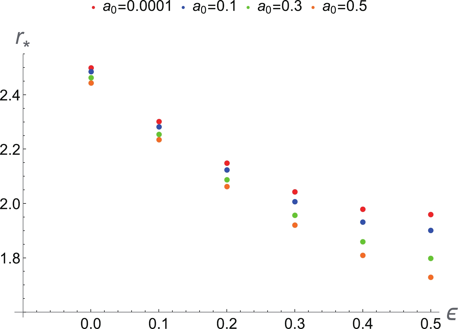
Figure 2. (color online) Relation between
$ r_* $ and$ \epsilon $ for different$ a_0 $ in the spherical accretion process for the ultra-relativistic fluid ($ w = 1/2 $ ).The phase space portrait of this dynamical system for the ultra-relativistic fluid with
$ M = 1 $ ,$ a_0 = 0.0001 $ , and$ \epsilon = 0.1 $ for a general parameterized black hole is depicted in Fig. 3, in which the physical flow of the ultra-relativistic fluid for a general parameterized black hole is represented by several curves. Clearly, both the critical points in Fig. 3,$ (r_*, v_*) $ and$ (r_*, -v_*) $ , are saddle points of the dynamical system. The five curves in Fig. 3 correspond to the different values of the Hamiltonian$ {\cal H}_0 = \{{\cal H}_*-0.05,\; {\cal H}_*- 0.02,\; {\cal H}_*,\; {\cal H}_*+ 0.03,\; {\cal H}_*+ 0.08\} $ . This plot shows several different types of fluid motion. The magenta (with$ {\cal H} = {\cal H}_* +0.08 $ ) and blue (with$ {\cal H} = {\cal H}_* +0.03 $ ) curves correspond to the purely supersonic accretion ($ v <- v_* $ branches), purely supersonic outflow ($ v > v_* $ branches), or purely subsonic accretion followed by the subsonic outflow ($ -v_*< v < v_* $ branches). The red (with$ {\cal H} = {\cal H}_* -0.02 $ ) and green (with$ {\cal H} = {\cal H}_* -0.05 $ ) curves correspond to the non-physical behavior of the fluid.
Figure 3. (color online) Phase space portrait of the dynamical system (33), (34) for the ultra-relativistic fluid (
$ w = 1/2 $ ), for the black hole parameters$ M = 1 $ ,$ \epsilon = 0.1 $ , and$ a_0 = 0.0001 $ . The critical (sonic) points$ (r_*, \pm v_*) $ of this dynamical system are presented by the black spots in the figure. The five colored curves (black, red, green, magenta, and blue) correspond to the Hamiltonian values$ {\cal H} = {\cal H}_*,\; {\cal H_*}-0.02, {\cal H}_*- 0.05, {\cal H}+0.03, {\rm{and}}\ {\cal H}_* + 0.08 $ .The most interesting solution of the fluid motion is depicted by the black curves in Fig. 3, revealing the transonic behavior of the fluid outside the black hole horizon. For
$ v<0 $ , there are two black hole curves that go through the sonic point$ (r_*, -v_*) $ . One solution starts at the spatial infinity with a sub-sonic flow followed by a supersonic flow after it crosses the sonic point, which corresponds to the standard nonrelativistic accretion considered by Bondi in [4]. Another solution, which starts at the spatial infinity with a supersonic flow but becomes sub-sonic after it crosses the sonic point, is unstable, according to the analysis presented in [46]; such a behavior is very difficult to achieve. For$ v>0 $ , there are two solutions as well. One solution, which starts at the horizon with a supersonic flow followed by a sub-sonic flow after it crosses the sonic point, corresponds to the transoinc solution of the stellar wind, as discussed in [4] for the non-relativistic accretion. Another solution, similar to the$ v<0 $ case, is unstable and too difficult to achieve [46].Here, we would like to add several remarks about the physical explanations of the flows in Fig. 3 for different values of Hamiltonian
$ {\cal H} $ . In general, different values of the Hamiltonian represent different initial states of the dynamical system. For the transonic solution of the ultra-relativistic fluid, its Hamiltonian can be evaluated at the sonic point. The Hamiltonian with values different from the transonic one does not represent any transonic solutions of the flow. For example, the green curve shows the subcritical fluid flow since such a flow does not pass through the critical point and fails to reach the critical point. In fact, such solutions have a turning or bouncing point, which is the nearest point reachable by such fluids, beyond which they are bounced back or turned around to infinity. A similar explanation holds for the red curves. The curves shown in blue and magenta can be termed super-critical flows. Although such fluids do not go through the critical point either, they already possess velocities above the allowed critical value. Such flows end up entering the black horizon. It is also worth mentioning that a similar analysis also applies to other fluids, including radiation, sub-relativistic, and polytropic fluids. -
For a radiation fluid, the equation of state is
$ w = 1/3 $ . In this case, the Hamiltonian (48) becomes$ {\cal H} = \frac{\left(1-\dfrac{2M}{r(1+\epsilon)}\right)^{2/3} \left[1+\dfrac{4 M^2 (a_0- \epsilon)}{r^2 (1+\epsilon)^2} - \dfrac{2 M \epsilon }{r(1+\epsilon)}\right]^{2/3}}{r^{4/3}|v|^{2/3} (1-v^2)^{2/3} }, $

(61) and then, the two-dimensional dynamical system (33), (34) is
$ \begin{aligned}[b] \dot{r} = &\frac{4 v^{1/3} \left(1 - \dfrac{2 M}{r (1 +\epsilon)}\right)^{2/3} \left[1 + \dfrac{ 4 M^2 (a_0 - \epsilon)}{r^2 (1 + \epsilon)^2} - \dfrac{ 2 M \epsilon}{r (1 + \epsilon)}\right]^{2/3}}{3 r^{ 4/3} (1 - v^2)^{5/3}} \\ &-\frac{2 \left(1 - \dfrac{2 M}{r (1 +\epsilon)}\right)^{2/3} \left[1 + \dfrac{ 4 M^2 (a_0 - \epsilon)}{r^2 (1 + \epsilon)^2} - \dfrac{ 2 M \epsilon}{r (1 + \epsilon)}\right]^{2/3}}{3 r^{ 4/3}|v|^{5/3} (1 - v^2)^{5/3}}, \end{aligned} $

(62) $ \begin{aligned}[b] \dot{v} = &\frac{4\left(1-\dfrac{2M}{r(1+\epsilon)}\right)^{2/3} \left[1+\dfrac{4 M^2 (a_0- \epsilon)}{r^2 (1+\epsilon)^2} - \dfrac{2 M \epsilon }{r(1+\epsilon)}\right]^{2/3}}{3 r^{7/3}|v|^{2/3}(1-v^2)^{2/3} } \\ & - \frac{2\left(1-\dfrac{2M}{r(1+\epsilon)}\right)^{} \left[-\dfrac{8 M^2 (a_0- \epsilon)}{r^3 (1+\epsilon)^2} + \dfrac{2 M \epsilon }{r^2 (1+\epsilon)}\right]^{}}{ LT_3} \\ &-\frac{4 M \left(1 + \dfrac{4 M^2 (a_0 - \epsilon)}{r^2 (1 + \epsilon)^2} - \dfrac{2 M\epsilon}{r (1 + \epsilon)}\right)}{r^2 (1 + \epsilon) LT_3}, \end{aligned} $

(63) where
$\begin{aligned}[b] LT_3 =& 3 r^{4/3} |v|^{2/3} (1-v^2)^{2/3} \left(1-\frac{2M}{r(1+\epsilon)}\right)^{1/3}\\&\times\left[1+\frac{4 M^2 (a_0- \epsilon)}{r^2 (1+\epsilon)^2} - \frac{2 M \epsilon }{r(1+\epsilon)}\right]^{1/3}. \end{aligned} $

(64) The sonic points can be found by solving the above two-dimensional dynamical system, when both right hand sides of Eq. (62) and Eq. (63) vanish. The values of the critical radius
$ r_* $ , sound speed$ \pm v_* $ , and critical$ {\cal H}_* $ for different values of$ \epsilon $ are summarized in Table 3 for$ w = 1/3 $ ,$ M = 1 $ , and$ a_0 = 0.0001 $ . Similar to the ultra-relativistic fluid, the critical radius decreases with increasing$ \epsilon $ , while the critical Hamiltonian$ {\cal H}_* $ increases. We also illustrate the behavior of the critical radius$ r_* $ for the radiation fluid with respect to$ \epsilon $ for different values of$ a_0 $ in Fig. 4.$ \epsilon $ 

$ 0 $ 

$ 0.1 $ 

$ 0.2 $ 

$ 0.3 $ 

$ 0.4 $ 

$ 0.5 $ 

$ r_0 $ 

$ 2 $ 

$ 1.81818 $ 

$ 1.66667 $ 

$ 1.53846 $ 

$ 1.42857 $ 

$ 1.33333 $ 

$ r_* $ 

$ 2.99996 $ 

$ 2.8096 $ 

$ 2.67692 $ 

$ 2.59413 $ 

$ 2.55246 $ 

$ 2.54108 $ 

$ v_* $ 

$ 0.57735 $ 

$ 0.57735 $ 

$ 0.57735 $ 

$ 0.57735 $ 

$ 0.57735 $ 

$ 0.57735 $ 

$ {\cal H}_* $ 

$ 0.20999 $ 

$ 0.22082 $ 

$ 0.22845 $ 

$ 0.23316 $ 

$ 0.2355 $ 

$ 0.23613 $ 

Table 3. Values of
$ r_* $ ,$ v_* $ , and$ {\cal H}_* $ at the sonic point, for different values of the black hole parameter$ \epsilon $ for the radiation fluid with$ w=1/3 $ . We use$ M=1 $ and$ a_0 = 0.0001 $ in the calculation.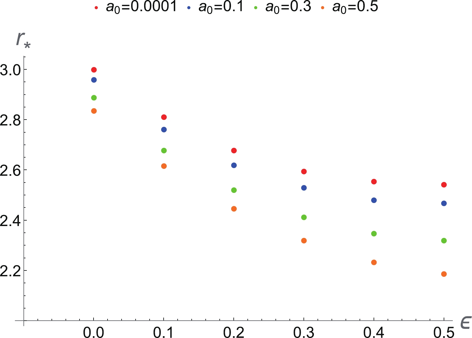
Figure 4. (color online) Relation between
$ r_* $ and$ \epsilon $ for different$ a_0 $ in the spherical accretion process for the radiation fluid ($ w = 1/3 $ ).The phase space portrait of this dynamical system for the radiation fluid with
$ M = 1 $ ,$ a_0 = 0.001 $ , and$ \epsilon = 0.1 $ is displayed in Fig. 5, in which the physical flow of the radiation fluid for a general parameterized black hole is represented by several curves. One can see that both the critical points in Fig. 5,$ (r_*, v_*) $ and$ (r_*, -v_*) $ , are saddle points of the dynamical system. From Fig. 5, one also observes that the radiation fluid shares the same types of the fluid motion ($ w = 1/3 $ ) as the ultra-relativistic fluid ($ w = 1/2 $ ), as shown in Fig. 3. Similar to Fig. 3, the magenta and blue curves represent the supersonic flows for$ v<-v_* $ or$ v>v_* $ , while they correspond to sub-sonic flows if$ -v_* < v< v_* $ . The transonic solutions are presented by the black curves. For$ v<0 $ , one of the black curves, which starts at the spatial infinity with a sub-sonic flow and then becomes supersonic after it crosses the sonic point$ (r_*, -v_*) $ , corresponds to the standard transonic accretion, and another black curve represents an unstable solution. For$ v>0 $ , one black curve corresponds to the transonic outflow of wind, and another one represents an unstable flow, similar to the case of the ultra-relativistic fluid. The green and red curves are non-physical solutions.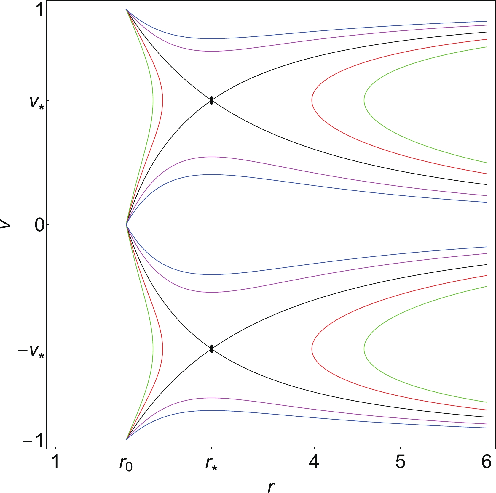
Figure 5. (color online) Phase space portrait of the dynamical system (33), (34) for the radiation fluid (
$ w = 1/3 $ ) for black hole parameters$ M = 1 $ ,$ \epsilon = 0.1 $ , and$ a_0 = 0.0001 $ . The critical (sonic) points$ (r_*, \pm v_*) $ of this dynamical system are presented by the black spots in the figure. The five colored curves (black, red, green, magenta, and blue) correspond to the values of Hamiltonian$ {\cal H} = {\cal H}_*,\; {\cal H_*}-0.03, {\cal H}_*- 0.05, {\cal H}+0.05, {\rm{and}}\ {\cal H}_* + 0.1 $ , respectively. -
Let us now consider a sub-relativistic fluid, whose energy density exceeds its isotropic pressure; the equation of state for such a fluid is
$ w = 1/4 $ . In this case, the Hamiltonian (48) takes the form$ {\cal H} = \frac{\left(1-\dfrac{2M}{r(1+\epsilon)}\right)^{3/4} \left[1+\dfrac{4 M^2 (a_0- \epsilon)}{r^2 (1+\epsilon)^2} - \dfrac{2 M \epsilon }{r(1+\epsilon)}\right]^{3/4}}{r\sqrt{|v|}(1-v^2)^{3/4}} , $

(65) and then the two-dimensional dynamical system is
$ \begin{aligned}[b] \dot{r} = &\frac{3\sqrt{ |v|} \left(1 - \dfrac{2 M}{r (1 +\epsilon)}\right)^{3/4} \left[1 + \dfrac{ 4 M^2 (a_0 - \epsilon)}{r^2 (1 + \epsilon)^2} - \dfrac{ 2 M \epsilon}{r (1 + \epsilon)}\right]^{3/4}}{2r^{} (1 - v^2)^{7/4}} \\ &-\frac{ \left(1 - \dfrac{2 M}{r (1 +\epsilon)}\right)^{3/4} \left[1 + \dfrac{ 4 M^2 (a_0 - \epsilon)}{r^2 (1 + \epsilon)^2} - \dfrac{ 2 M \epsilon}{r (1 + \epsilon)}\right]^{3/4}}{ r^{}|v|^{3/2} (1 - v^2)^{3/4}}, \\[-15pt] \end{aligned} $

(66) $ \begin{aligned}[b] \dot{v} = &\frac{\left(1-\dfrac{2M}{r(1+\epsilon)}\right)^{3/4} \left[1+\dfrac{4 M^2 (a_0- \epsilon)}{r^2 (1+\epsilon)^2} - \dfrac{2 M \epsilon }{r(1+\epsilon)}\right]^{3/4}}{ r^{2}\sqrt{|v|}(1-v^2)^{3/4} } \\ &- \frac{3\left(1-\dfrac{2M}{r(1+\epsilon)}\right)^{} \left[-\dfrac{8 M^2 (a_0- \epsilon)}{r^3 (1+\epsilon)^2} + \dfrac{2 M \epsilon }{r^2 (1+\epsilon)}\right]^{}}{ LT_4} \\ &-\frac{4 M \left(1 + \dfrac{6 M^2 (a_0 - \epsilon)}{r^2 (1 + \epsilon)^2} - \dfrac{2 M\epsilon}{r (1 + \epsilon)}\right)}{r^2 (1 + \epsilon) LT_4}, \end{aligned} $

(67) where
$\begin{aligned}[b] LT_4 =& 4 r \sqrt{|v|} (1-v^2)^{3/4} \left(1-\frac{2M}{r(1+\epsilon)}\right)^{1/4}\\&\times\left[1+\frac{4 M^2 (a_0- \epsilon)}{r^2 (1+\epsilon)^2} - \frac{2 M \epsilon }{r(1+\epsilon)}\right]^{1/4}. \end{aligned}$

(68) For this dynamical system, similar to the above two cases, we present the values of
$ r_* $ ,$ v_* $ , and$ {\cal H}_* $ for different values of$ \epsilon $ in Table. 4 for$ w = 1/4 $ ,$ M = 1 $ , and$ a_0 = 0.0001 $ . We also plot the behavior of the critical radius$ r_* $ for the sub-relativistic fluid with respect to the black hole parameter$ \epsilon $ for different values of$ a_0 $ ; this is shown in Fig. 6. Clearly, the critical radius$ r_* $ decreases with increasing$ \epsilon $ and$ a_0 $ .$ \epsilon $ 

$ 0 $ 

$ 0.1 $ 

$ 0.2 $ 

$ 0.3 $ 

$ 0.4 $ 

$ 0.5 $ 

$ r_0 $ 

$ 2 $ 

$ 1.81818 $ 

$ 1.66667 $ 

$ 1.53846 $ 

$ 1.42857 $ 

$ 1.33333 $ 

$ r_* $ 

$ 3.49993 $ 

$ 3.32303 $ 

$ 3.20741 $ 

$ 3.13980 $ 

$ 3.10743 $ 

$ 3.09881 $ 

$ v_* $ 

$ 0.5 $ 

$ 0.5 $ 

$ 0.5 $ 

$ 0.5 $ 

$ 0.5 $ 

$ 0.5 $ 

$ {\cal H}_* $ 

$ 0.26557 $ 

$ 0.27281 $ 

$ 0.27750 $ 

$ 0.28022 $ 

$ 0.2815 $ 

$ 0.28184 $ 

Table 4. Values of
$ r_* $ ,$ v_* $ , and$ {\cal H}_* $ at the sonic point, for different values of the black hole parameter$ \epsilon $ for the sub-relativistic fluid$ w=1/4 $ . The black hole parameters M and$ a_0 $ are set to$ M=1 $ and$ a_0 = 0.0001 $ .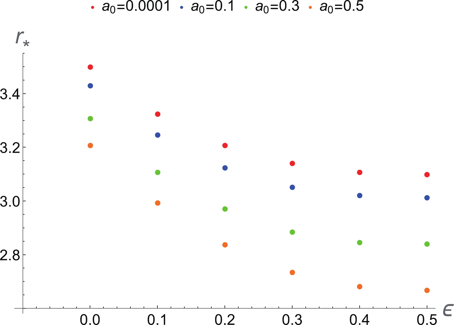
Figure 6. (color online) Relation between
$ r_* $ and$ \epsilon $ for different$ a_0 $ in the spherical accretion process for the sub-relativistic fluid ($ w=1/4 $ ).The phase space portrait of the dynamical system for the sub-relativistic fluid is shown in Fig. 7. From this figure, we observe that the type of the fluid motion for the sub-relativistic fluid (
$ w = 1/4 $ ) is same as those for the ultra-relativistic fluid ($ w = 1/2 $ ) and the radiation fluid ($ w = 1/3 $ ). For$ v>v_* $ , the magenta and blue curves are purely supersonic outflows, while for$ v<-v_* $ , they represent supersonic accretions. For$ -v_* < v < v_* $ , these curves are sub-sonic flows. The black curves shown in Fig. 7 are more interesting since they represent the transonic solution of the spherical accretion for$ v<0 $ and spherical outflow for$ v>0 $ around the black hole. Similar to the results for the ultra-relativistic and radiation fluids, the red and green curves represent non-physical solutions.
Figure 7. (color online) Phase space portrait of the dynamical system (33), (34) for the sub-relativistic fluid (
$ w = 1/4 $ ), for the black hole parameters$ M = 1 $ ,$ \epsilon = 0.1 $ , and$ a_0 = 0.0001 $ . The parameters are$ r_0 \simeq 1.81818 $ ,$ r_* \simeq 3.32303 $ ,$ v_* \simeq 0.5 $ . Black plot: the solution curve through the saddle CPs ($ r_*, v_* $ ) and ($ r_*, -v_* $ ) for which$ {\cal H} = {\cal H}_* \simeq 0.272806 $ . Red plot: the solution curve for which$ {\cal H} = {\cal H}_*- 0.03 $ . Green plot: the solution curve for which$ {\cal H} = {\cal H}_*- 0.05 $ . Magenta plot: the solution curve for which$ {\cal H} = {\cal H}_* + 0.03 $ . Blue plot: the solution curve for which$ {\cal H} = {\cal H}_* + 0.1 $ . -
The state of a polytropic test fluid can be described by
$ p = \kappa n^\gamma , $

(69) where
$ \kappa $ and$ \gamma $ are constants. For ordinary matter, one generally works with the constraint$ \gamma > 1 $ . Following [45], we obtain the following expressions for the specific enthalpy:$ h = m +\frac{\kappa \gamma n^{\gamma -1}}{\gamma - 1}, $

(70) where the constant of integration has been identified with the baryonic mass m. The three-dimensional speed of sound is given by
$ c_s^2 = \frac{(\gamma -1) Y}{m(\gamma -1) + Y}\; \; \; (Y \equiv \kappa \gamma n^{\gamma -1}). $

(71) Using Eq. (41) in Eq. (71), we obtain
$ h = m\left[ 1+ Z \left(\frac{1-v^2}{r^4 N^2 v^2}\right)^{(\gamma -1)/2}\right], $

(72) where
$ Z \equiv \frac{\kappa \gamma}{m(\gamma -1)} \left| C_1 \right|^{\gamma - 1} = {\rm{const}}.>0, $

(73) and Z is a positive constant. If critical points exist, Z takes the special form
$ Z \equiv \frac{\kappa \gamma n^{\gamma -1}_*}{m(\gamma -1)} \left(\frac{r^5_* N^2_{*,r_*}}{4}\right)^{(\gamma - 1)/2} = {\rm{const}}.>0 . $

(74) The constant Z depends on the black hole parameters and the test fluid. From Eq. (74), it is clear that Z is roughly proportional to
$ \kappa n_* / m $ for a given black hole solution and certain test fluids.Inserting Eq. (72) into Eq. (31), we evaluate the Hamiltonian by
$ {\cal H} = \frac{N^2}{1 - v^2}\left[1 + Z \left( \frac{1 - v^2}{r^4 N^2 v^2}\right)^{(\gamma -1)/2}\right]^2, $

(75) where
$ m^2 $ has been absorbed into a redefinition of$ (\bar{t},{\cal H}) $ . Obviously,$ N^2(r) >0 $ and$ N^2_{,r} > 0 $ for all r. This means that the constant$ Z >0 $ (recall that$ \gamma >1 $ ). It is easy to see that there are no global solutions, since the Hamiltonian remains constant along the solution curves.Notice that since
$ \gamma > 1 $ , the solution curves do not cross the r axis at points where$ v = 0 $ and$ r \ne r_0 $ ; otherwise, the Hamiltonian (75) would diverge there. The point on the r axis which the solution curves may cross is only$ (r_0,0) $ . The horizon$ r = r_0 $ is a single root to$ N^2(r) = 0 $ , in the vicinity of which v behaves as$ \left|v\right| \propto \left| r-r_0\right|^{\textstyle\frac{2-\gamma}{2(\gamma -1)}}. $

(76) We see that only solutions with
$ 1<\gamma< 2 $ may cross the r axis. Here,$ {\cal H}(r_0,0) $ is the limit of$ {\cal H}(r,v) $ as$ (r,v) $ $ \to $ $ (r_0,0) $ . When$ 1<\gamma< 2 $ , the pressure$ p = \kappa n^\gamma $ diverges at the horizon as$ p \propto \left| r-r_0\right|^{\textstyle\frac{-\gamma}{2(\gamma -1)}}. $

(77) Then, inserting
$ Y = m(\gamma-1) Z \left(\frac{1-v^2}{r^4 N^2 v^2}\right)^{(\gamma -1)/2} $

(78) into Eq. (71), we obtain
$ c_s^2 = Z (\gamma -1- c_s^2) \left(\frac{1-v^2}{r^4 N^2 v^2}\right)^{(\gamma -1)/2} . $

(79) This, along with Eq. (36), takes the form of the following expressions at the critical points (
$ c_s^2(r_*) = $ $ v^2(r_*) = v^2_* $ ):$ c_s^2(r_*) = Z (\gamma -1- v^2_*) \left(\frac{1-v^2_*}{r^4_* N^2_* v^2_*}\right)^{(\gamma -1)/2}, \; $

(80) $ v^2_* = \frac{M [-12 M^2 \epsilon + r_*^2 (1 + \epsilon)^3 + 4 a_0 M (3 M - r_* (1 + \epsilon))]}{LT_1}. $

(81) Here, we have used Eq. (36) to obtain the right-hand side of Eq. (81). If there are critical points, the solution of this system of equations in
$ (r_*,v_*) $ provides all the critical points, with a given value of the positive constant Z. Then, one can use the values of critical points to reduce$ n_* $ from Eq. (74).Numerical solutions to the dynamical system of Eqns. (80) and (81) are shown in Fig. 8. Clearly, there is only one critical point, a saddle point, in accretion (
$ -1<v<0 $ ) of a polytropic test fluid. The motion types for the polytropic test fluids, as shown in Fig. 8, are the same as the motion types for the isothermal test fluids with$ w = 1/2 $ (c.f. Fig. 3),$ w = 1/3 $ (c.f. Fig. 5), and$ w = 1/4 $ (c.f. Fig. 7).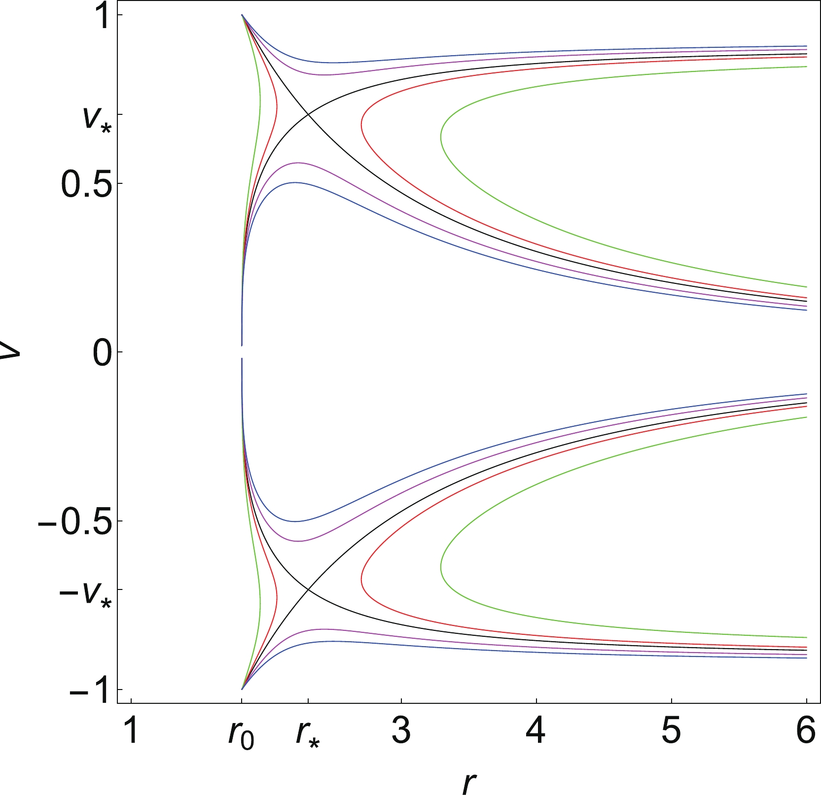
Figure 8. (color online) Accretion of a polytropic test fluid. Contour plots of the Hamiltonian (75) for
$ \gamma = 5/3 $ and$ Z = 5 $ , for the black hole parameters$ M = 1 $ ,$ \epsilon = 0.1 $ , and$ a_0 = 0.0001 $ . The parameters are$ r_0 \simeq 1.81818 $ ,$ r_* \simeq 2.30998 $ ,$ v_* \simeq 0.704098 $ . Black plot: the solution curve through the saddle CPs ($ r_*, v_* $ ) and ($ r_*, -v_* $ ) for which$ {\cal H} = {\cal H}_* \simeq 5.5208 $ . Red plot: the solution curve for which$ {\cal H} = {\cal H}_*-0.3 $ . Green plot: the solution curve for which$ {\cal H} = {\cal H}_*-1.0 $ . Magenta plot: the solution curve for which$ {\cal H} = {\cal H}_*+0.5 $ . Blue plot: the solution curve for which$ {\cal H} = {\cal H}_*+1.0 $ -
Recently, a correspondence was shown between the sonic points of the ideal photon gas and the photon sphere in static spherically symmetric spacetimes [37]. This important result is valid not only for spherical accretion of the ideal photon gas but also for rotating accretion in static spherically symmetric spacetimes [38, 39, 47]. In this section, we establish this correspondence for parameterized spherically symmetric black holes.
Let us first consider the spherical accretion of the ideal photon gas and derive the corresponding sonic points. The equation of state for the ideal photon gas in d-dimensional space is
$ h = \frac{k \gamma}{\gamma -1} n^{\gamma -1}, $

(82) with
$ \gamma = \frac{d+1}{d}, $

(83) where k is a constant of the entropy [37]. The speed of sound for the ideal photon gas is constant
$ c_s^2 \equiv \frac{{\rm d} \ln h }{{\rm d} \ln n} = \gamma -1. $

(84) For general parameterized spherically symmetric spacetimes (
$ d = 3 $ ), the equation of state of the ideal photon gas becomes$ h = 4 k n^{1/3}, $

(85) and the speed of sound for the ideal photon gas is
$ c_s^2 = 2 $ . For the accretion of the ideal photon gas in parameterized spherically symmetric spacetimes, the radius$ r_* $ of the sonic point is specified by$ \frac{\rm d }{{\rm d} r}\left(\frac{N}{r}\right) = 0. $

(86) To proceed, let us derive the photon sphere by analyzing the evolution of a photon in a parameterized spherically symmetric black hole. The photon follows the null geodesics in a given black hole spacetime. As the spacetime is spherically symmetric, we can perform the calculations in the equatorial plane
$ \theta = \pi/2 $ . To find the null geodesics around the black hole we can use the Hamilton-Jacobi equation, given as follows:$ \frac{\partial S}{\partial \lambda} = -\frac{1}{2}g^{\mu\nu}\frac{\partial S}{\partial x^\mu}\frac{\partial S}{\partial x^\nu}, $

(87) where
$ \lambda $ is the affine parameter of the null geodesic, and S denotes the Jacobi action of the photon. The Jacobi action S can be separated in the following form:$ S = -Et+L\phi+S_r(r), $

(88) where E and L represent the energy and the angular momentum of the photon, respectively. The function
$ S_r(r) $ depends only on r.Substituting the Jacobi action into the Hamilton-Jacobi equation, we obtain
$ S_r(r) = \int^r\frac{B^2(r)\sqrt{R(r)}}{r^2 N^2(r)}{\rm d}r, $

(89) where
$ R(r)= -\frac{r^2 N^2(r)L^2}{B^2(r)}+\frac{r^4 E^2}{B^2(r)}. $

(90) The variation of the Jacobi action gives the following equations of motion for the evolution of the photon:
$ \frac{{\rm d}t}{{\rm d}\lambda} = \frac{E}{N^2(r)}, $

(91) $ \frac{{\rm d}\phi}{{\rm d}\lambda} =\frac{L}{r^2}, $

(92) $ \frac{{\rm d}r}{{\rm d}\lambda} = \frac{\sqrt{R(r)}}{r^2}. $

(93) To determine the radius of the photon sphere of the black hole, we need to find the critical circular orbit for the photon, which can be derived from the unstable condition
$ R(r) = 0,\qquad \frac{{\rm d}R(r)}{{\rm d}r} = 0. $

(94) For a parameterized spherically symmetric black hole, from the above conditions, one finds
$ \frac{\rm d}{{\rm d}r}\left(\frac{N}{r}\right) = 0. $

(95) This is the condition for determining the radius of the photon sphere. Clearly, Eq. (86) is actually the same as Eq. (95), which means that the critical radius
$ r_* $ of a sonic point, for the accretion of the ideal photon gas in parameterized spherically symmetric spacetimes, is equal to the radius of the photon sphere.With Eq. (95), one obtains the critical radius
$ r_* $ and the radius of the photon sphere in parameterized spherically symmetric spacetimes$ r_* = \left. \left(\frac{1}{N} \frac{{\rm d} N}{{\rm d}r} \right)^{-1} \right|_{r = r_*}. $

(96) By substituting Eq. (47) into the above equation, we obtain the expression for
$ r_* $ ,$\begin{aligned}[b] r_* =& M + \frac{(1 + {\rm{i}} \sqrt{3}) M^2 (1 + \epsilon) [-8 a_0 + 3 (1 + \epsilon)^2]}{2LT_{5}} \\&+ \frac{(1 - {\rm{i}} \sqrt{3}) LT_{5}}{6 (1 + \epsilon)^3}, \end{aligned}$

(97) where
$\begin{aligned} LT_{5} =& [-27 M^3 (1 + \epsilon)^6 (1 + a_0 (6 - 4 \epsilon) - 7 \epsilon + 3 \epsilon^2 + \epsilon^3)\\& + 6 \sqrt{3} \sqrt{LT_{6} }]^{1/3},\end{aligned}$

(98) and
$ \begin{aligned}[b] LT_{6} = &M^6 (1 + \epsilon)^{12} [128 a_0^3 - 9 a_0^2 (-11 + 68 \epsilon + 4 \epsilon^2) \\ &- 135 \epsilon (1 - 2 \epsilon + 3 \epsilon^2 + \epsilon^3) + 135 a_0 (1 - 3 \epsilon + 7 \epsilon^2 + \epsilon^3)]. \end{aligned}$

(99) It is easy to verify that when the additional parameters (
$ a_0 $ and$ \epsilon $ ) are set to zero, the critical radius reduces to$ r_* = 3M $ . In Fig. 9, we schematically show the spherical accretion of the ideal photon gas onto a spherically symmetric black hole and its photon sphere (represented by the red circle). The red circle in Fig. 9 thus has a two-fold meaning, since it represents both the photon sphere and the sonic radius of the spherical accretion of the ideal photon gas.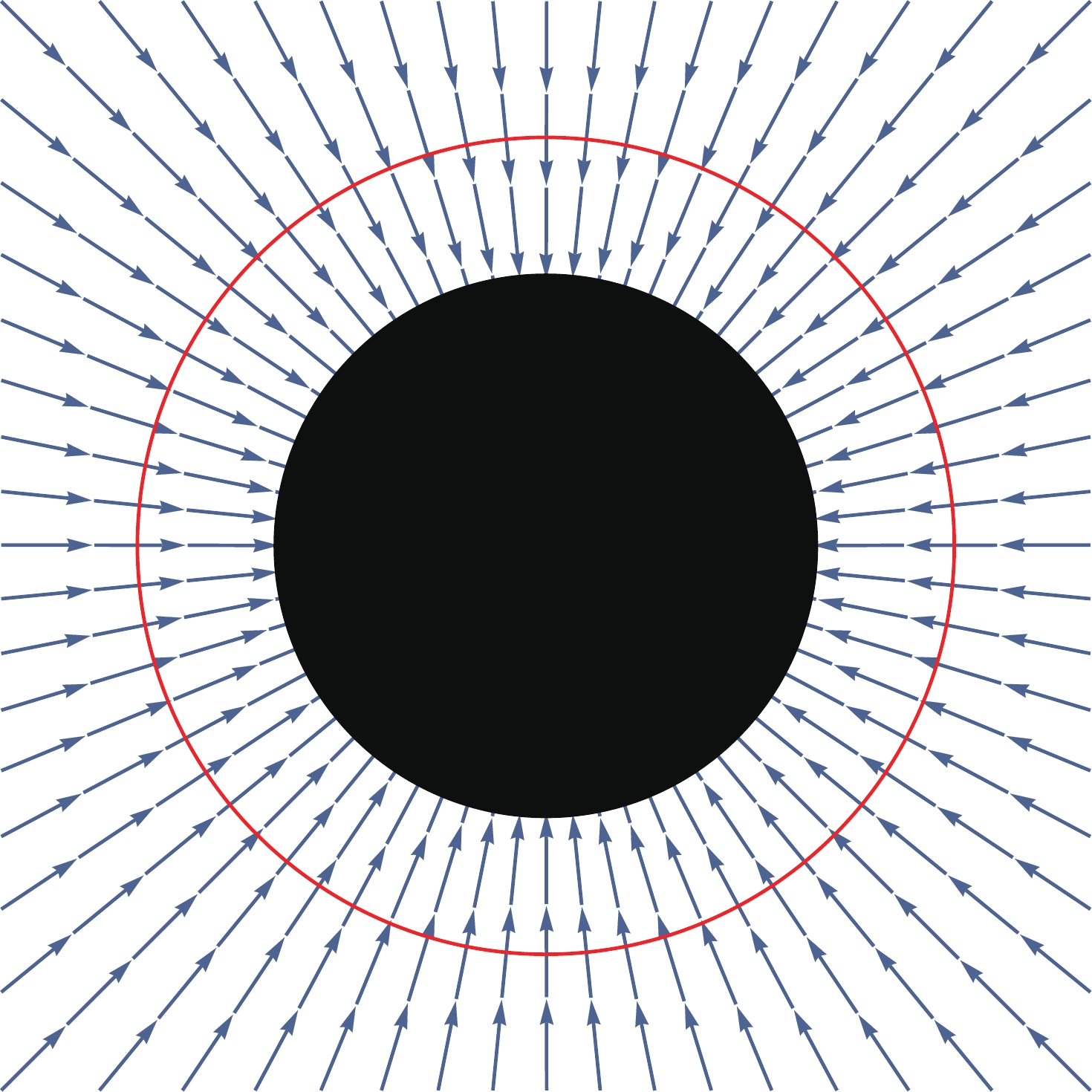
Figure 9. (color online) Schematic of the spherical accretion of the ideal photon gas onto a spherically symmetric black hole and its photon sphere (the red circle). The red circle has a two-fold meaning, since it represents both the photon sphere and the sonic radius of the spherical accretion of the ideal photon gas.
-
In this paper, we studied the spherical accretion flow of a perfect fluid onto a general parameterized spherically symmetric black hole. For this purpose, we first formulated two basic equations for describing the accretion process and presented the general formulas for determining the sonic points (or critical points). These two equations were derived from the conservation laws of energy and particle number of the fluid. Using these two equations, we analyzed the accretion processes of various perfect fluids, such as the isothermal fluids of the ultra-stiff, ultra-relativistic, and sub-relativistic types, and polytropic fluids. The flow behaviors of these test fluids around a general parameterized spherically symmetric black hole were studied in detail and are shown graphically in Figs. 1, 3, 5, 7. For the isothermal fluid, it is interesting to mention that the sonic point does not exist for the ultra-stiff fluid with
$ w = 1 $ alone; thus, transonic solutions exist for the ultra-relativistic fluid with$ w = 1/2 $ , for the radiation fluid with$ w = 1/3 $ , and for the sub-relativistic fluid$ w = 1/4 $ . The value of$ \epsilon $ affects$ r_0,\; r_*,\; {\rm and}\ {\cal H}_* $ but not$ v_* $ , which indicates the effect of the position of the event horizon. For the polytropic fluid, Fig. 8 shows that it exhibits a similar flow behavior as the isothermal fluids with$ w = 1/2 $ ,$ w = 1/3 $ , and$ w = 1/4 $ . Here, we would like to mention that the results presented in this paper can also be reduced to specific cases in several modified theories of gravity. For example, one can map the results here to the first-type Einstein-Aether black hole in [48, 49] by setting$ \epsilon = \frac{M-\sqrt{M^2-{\text{æ}}^2}}{M+\sqrt{M^2-{\text{æ}}^2}}, $

(100) $ a_0 = \frac{{\text{æ}}^2}{(M+\sqrt{M^2-{\text{æ}}^2})^2}, \;\;\;\; b_0 = 0, $

(101) $ a_i = 0, \;\;\; b_i = 0, \;\;\;\; (i>0), $

(102) where
$ {\text{æ}}^2 = - \frac{2 c_{13}-c_{14}}{2(1-c_{13})} M^2, $

(103) with
$ c_{13} $ and$ c_{14} $ being the coupling constants in the Einstein-Aether theory. It is interesting to mention that flow behaviors for different test fluids in this paper are qualitatively consistent with those studied in [50] for the spherical accretion in the Einstein-Aether theory.We further considered the spherical accretion of the ideal photon gas and derived the radius of its sonic point. Comparing the radius with that of the photon sphere for a general parameterized spherically symmetric black hole, we studied the correspondence between the sonic points of the accreting photon gas and the photon sphere for a general parameterized spherically symmetric black hole.
With the above main results, we would like to mention several directions that can be pursued for extending our analysis. First, spherical accretion is the simplest accretion scenario, in which the accreting matter falls steadily and radially into a black hole. This is an extreme simple case. Therefore, it is interesting to explore the accreting behaviors of various types of matter when the spherical symmetry approximation is relaxed by considering a non-zero relative velocity between the black hole and the accreting matter. This scenario is also known as wind accretion or Bondi–Hoyle–Lyttleton accretion [51-53] (see [54] for a review). We will consider the more complicated accretion disk model, which is more related to real observations, in our future work.
Second, it is also interesting to extend our analysis to rotating black holes. In a rotating background, one may consider rotating fluids accreting onto a rotating black hole. The rotation of the fluids can lead to the formation of a disc-like structure around the black hole, and such accretion discs are the most commonly studied engines for explaining astrophysical phenomena such as active galactic nuclei, X-ray binaries, and gamma-ray bursts. However, considering rotation introduces complications into the accretion problem, in which case, the study heavily relies on numerical calculations.
Finally, when one considers a rotating black hole, its shadow does not correspond to a photon sphere but a photon region. An immediate question now arises as to what structure in the rotating accretion of the ideal photon gas corresponds to the photon region of a rotating black hole. This is still an open issue.
Spherical accretion flow onto general parameterized spherically symmetric black hole spacetimes
- Received Date: 2020-08-02
- Available Online: 2021-01-15
Abstract: The transonic phenomenon of black hole accretion and the existence of the photon sphere characterize strong gravitational fields near a black hole horizon. Here, we study the spherical accretion flow onto general parametrized spherically symmetric black hole spacetimes. We analyze the accretion process for various perfect fluids, such as the isothermal fluids of ultra-stiff, ultra-relativistic, and sub-relativistic types, and the polytropic fluid. The influences of additional parameters, beyond the Schwarzschild black hole in the framework of general parameterized spherically symmetric black holes, on the flow behavior of the above-mentioned test fluids are studied in detail. In addition, by studying the accretion of the ideal photon gas, we further discuss the correspondence between the sonic radius of the accreting photon gas and the photon sphere for general parameterized spherically symmetric black holes. Possible extensions of our analysis are also discussed.


 DownLoad: