


 Abstract
 HTML
HTML Reference
 Related
 PDF
PDF


-
The
$J/\psi$ meson, a bound state of a charm quark and its anti-particle, was discovered in 1974; since then, it has been studied extensively from a theoretical and experimental point of view. In heavy ion collisions at the RHIC [1] and recently at the LHC [2], its production mechanisms have been explored. Perhaps, the most significant phenomenon as a result of heavy ion collisions is formation of the particular state of matter called quark-gluon plasma (QGP). A fundamental effect associated with the QGP medium is known as color screening, i.e., the interaction range of heavy quarks decreases with an increase in the surrounding temperature [3]. As a result, the potential between heavier quarks$ c\bar{c} $ or$ b\bar{b} $ is screened due to the deconfinement of other quarks and gluons. The consequent separation of heavy quarks leads to suppressed quarkonium yields.$J/\psi$ suppression, an idea first put forward by theorists T. Matsui and H. Satz [4] in 1986, is considered one of the indicators of the formation of QGP. As charm quarks are more abundantly produced in heavy-ion experiments compared to bottom quarks, researchers initially thought that$ J/\psi $ could also be used to measure the temperature of QGP. However, due to technical issues associated with$ J/ \psi $ production, it is an unsuitable QGP temperature probe. Among J/$ \psi $ 's dominant decay modes is the production of lepton pairs. However, these dileptons do not possess the requisite momentum to carry them beyond the CMS particle spectrometer's large magnetic fields for detection. Furthermore, non-QGP effects can also play a role in the suppression of$J/ \psi $ . A better temperature probe that has been studied is the upsilon meson (bound state of bottom quark-anti quark) [5].Various papers have considered the dissociation of
$ J/\psi $ by light hadrons [6-15]. Due to the dominant scattering mechanism and the different assumptions made regarding it, the computed cross sections in these studies exhibit great variations at low energies. For example, Kharseev et al. [6, 7] studied the$ J/\psi $ -nucleon collision using the parton model and perturbative QCD "short distance" approach. The cross section they obtained at$ \sqrt{s} = 5 $ GeV was found to be approximately 0.25$\mu{\rm b}$ . Another study concerning the dissociation cross sections of$ J/\psi $ by$ \pi $ and$ \rho $ mesons was conducted by Matinyan and Muller [10]. At$ \sqrt{s} = 4 $ GeV, they obtained$ \sigma $ $ \approx $ 0.2-0.3${\rm mb}$ . The dissociation cross sections mentioned above attain particular significance once one considers the suppression of quarkonium states (such as the stronger$ \psi $ (2S) suppression relative to$ J/\psi $ ) due to the comover scattering effect [16, 17]. Other theoretical studies have also probed various phenomenological aspects related to$ J/\psi $ mesons.Lattice QCD calculations performed in [18-22] found a relatively narrow width of
$J/\psi$ , i.e., around 1.6$ T_{c} $ ($ T_{c} $ is known as the critical phase transition temperature). Subsequently, Wong [23] calculated the$J/\psi$ production cross section via charm quark-antiquark collision and showed the energy dependence of the cross section. Moreover, [23] concluded that, with the corresponding decrease in temperature, an increase in maximum cross section occurs. Theoretically, the two broad approaches used to study the dynamics of quarkonia are based on potential models and lattice QCD [24].Potential models assume that the gluonic field energy between a heavy quark and its corresponding antiquark can be modeled with the aid of a suitable potential. For a single quark-antiquark pair, the Cornell potential adequately describes the experimental results of quarkonium spectroscopy [25], agrees well with the lattice [26], and can be obtained via quantum chromodynamics (QCD) [27, 28]. This quark-antiquark system can be treated in the non-relativistic regime owing to the heavier quark mass (
$ m_{c,b} \gg \Lambda_{\rm{QCD}} $ ) and the low heavy quark velocity ($ v \ll 1 $ ). J. Weinstein and N. Isgur used the sum of two-body Cornell potentials in their study of$ K\bar{K} $ molecules [29, 30]. Subsequently, T. Barnes and E. Swanson employed the aforementioned approach [31] to compute the cross sections and elastic scattering phase shifts of$ \pi^{+}\pi^{+} $ ,$ K^{+}K^{+} $ , and$ \rho^{+}\rho^{+} $ .Another potential of interest to our current study is the quadratic potential. This has been widely used to probe nucleon-nucleon interaction [32-35] and, more recently, to calculate the mass spectra of tetraquarks [36]. Quadratic confinement has also been used to investigate a six-quark state with a structure akin to benzene [37].
In our study, we consider a system of two
$ J/\psi $ mesons and study their scattering cross sections with the aid of different potentials. We analyze how changing the potential between quarks changes the interaction between them. In Section II, we state the wavefunction of our system, followed by the Hamiltonian. The section ends with a discussion on quadratic and Cornell potentials. In Section III, integral equations are written and decoupled using the Born approximation. The final section is devoted to the results of the quadratic and Cornell potentials. -
We write the state function of our tetraquark system by utilizing the adiabatic approximation [38] as follows:
$ |\Psi_{T}\rangle = \sum\limits_{k = 1}^{2} \psi_{c}({\bf{Q}}_{c})\chi_{k}({\bf{Q}}_{k})\xi_{k}({\bf{u}}_{k})\zeta_{k}({\bf{v}}_{k})|k\rangle_{f}|k\rangle_{s}|k\rangle_{c}, $

(1) where
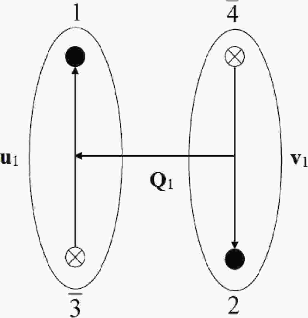
$ {\bf{Q}}_{c} $ : position of COM (center of mass) of our complete system,$ {\bf{Q}}_{1} $ : vector joining COM of (1,$ \bar{3} $ ) and (2,$ \bar{4} $ ) clusters,$ {\bf{u}}_{1} $ : vector representing position of quark 1 w.r.t. quark$ \bar{3} $ in the cluster (1,$ \bar{3} $ ),$ {\bf{v}}_{1} $ : vector representing position of quark 2 w.r.t. quark$ \bar{4} $ in the cluster (2,$ \bar{4} $ ).Identical expressions are given for clusters (1,
$ \bar{4} $ ) and (2,$ \bar{3} $ ) via$ {\bf{Q}}_{2} $ ,$ {\bf{u}}_{2} $ , and$ {\bf{v}}_{2} $ . Likewise, (1,2) and ($ \bar{3} $ ,$ \bar{4} $ ) are defined by$ {\bf{Q}}_{3} $ ,$ {\bf{u}}_{3} $ , and$ {\bf{v}}_{3} $ . Hence,$ \begin{aligned}[b] {\bf{Q}}_{1} =& \frac{1}{2}({\bf{\tau}}_{1} + {\bf{\tau}}_{\bar{3}} - {\bf{\tau}}_{2} -{\bf{\tau}}_{\bar{4}}) , \\ {\bf{u}}_{1} =& {\bf{\tau}}_{1} - {\bf{\tau}}_{\bar{3}} \ , \ {\bf{v}}_{1} = {\bf{\tau}}_{2} - {\bf{\tau}}_{\bar{4}} ,\end{aligned} $

(2) $ \begin{aligned}[b] {\bf{Q}}_{2} =& \frac{1}{2}({\bf{\tau}}_{1} + {\bf{\tau}}_{\bar{4}} - {\bf{\tau}}_{2} -{\bf{\tau}}_{\bar{3}}), \\ {\bf{u}}_{2} =& {\bf{\tau}}_{1} - {\bf{\tau}}_{\bar{4}} \ , \ {\bf{v}}_{2} = {\bf{\tau}}_{2} - {\bf{\tau}}_{\bar{3}} ,\end{aligned} $

(3) $ \begin{aligned}[b] {\bf{Q}}_{3} =& \frac{1}{2}({\bf{\tau}}_{1} + {\bf{\tau}}_{2} - {\bf{\tau}}_{\bar{3}} -{\bf{\tau}}_{\bar{4}}), \\ {\bf{u}}_{3} =& {\bf{\tau}}_{1} - {\bf{\tau}}_{2} \ , \ {\bf{v}}_{3} = {\bf{\tau}}_{\bar{3}} - {\bf{\tau}}_{\bar{4}}, \end{aligned} $

(4) $ \begin{aligned}[b] \xi_{k}({\bf{u}}_{k}) =& \frac{1}{(2\pi d^{2})^{3/4}} {\exp}\Bigg(\frac{- {\bf{u}}^{2}_{k}}{4d^{2}}\Bigg), \\ \zeta_{k}({\bf{v}}_{k}) =& \frac{1}{(2\pi d^{2})^{3/4}} {\exp}\Bigg(\frac{- {\bf{v}}^{2}_{k}}{4d^{2}}\Bigg). \end{aligned} $

(5) The possible topologies of quark-antiquark clusters are shown in Figures 1 and 2 respectively.

Figure 1. Topology A.
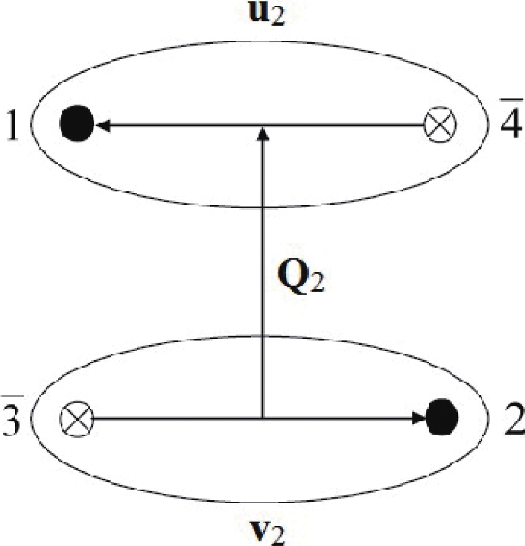
Figure 2. Topology B.
As we are considering the system in the COM reference frame,
$ \psi_{c}({\bf{Q}}_{c}) $ has no role in the dynamics of the four quark system.$ \chi_{k}({\bf{Q}}_{k}) $ is an unknown parameter in the radial part of the total wavefunction, and$ \xi_{k}({\bf{u}}_{k}) $ ,$ \zeta_{k}({\bf{v}}_{k}) $ are the predefined Gaussian wave functions.$ |k\rangle_{f} $ ,$ |k\rangle_{s} $ , and$ |k\rangle_{c} $ are the flavor, spin, and color parts of the wave function, respectively. The Hamiltonian of our (${{c\bar cc\bar c}}$ ) system is written as follows:$ \hat{H} = \sum\limits_{i = 1}^{\bar{4}} \bigg[m_{i} + \frac{\hat{P}_{i}^{2}}{2m_{i}}\bigg] + \sum\limits_{i<j}^{\bar{4}} [v(r_{ij})\bf{F_{i}}.\bf{F_{j}}] , $

(6) where m and
$ \hat{P} $ denote the quark mass and linear momentum, respectively. Moreover,$ F_{i} = \lambda_{i}/2 $ for a quark and$ F_{i} = - \lambda_{i}^{*}/2 $ for an antiquark, where$ \lambda $ s are the well-known Gell-Mann matrices. The potentials$ v(r_{ij}) $ used for$ q\bar{q} $ pairwise interaction are the quadratic potential [39],$ v_{ij} = Cr^{2}_{ij} + \bar{C}, $

(7) where
$ i,j = 1,2,\bar{3},\bar{4} $ , and the Cornell potential (Coulombic plus linear potential) [29] is$ v_{ij} = - \frac{4}{3} \frac{\alpha_{s}}{r_{ij}} + b_{s}r_{ij}, $

(8) where
$ i,j = 1,2,\bar{3},\bar{4} $ ,$ \alpha_{s} $ is the strong coupling constant, and$ b_{s} $ is the string tension (flux tube model).The mesonic size d appearing in
$ \xi_{k}({\bf{u}}_{k}) $ and$ \zeta_{k}({\bf{v}}_{k}) $ can be adjusted such that the Gaussian ground state wave function of the quadratic potential approximates the ground state wave function of the Cornell potential. Hence, their overlaps become unity for a fitted value of parameter d [40]. -
We employ the RGM (resonating group method) technique [41] and take variations only in the
$ \chi_{k} $ $ ({\bf{Q}}_{k}) $ factor of the total wave function$ \Psi_{T} $ ; by making use of linear independence of these variations both w.r.t. the two values of k, i.e., k = 1, 2, and w.r.t. all possible continuous values of$ {\bf{Q}}_{k} $ in$ \langle \delta \Psi_{T}| H - E_{c}|\Psi_{T}\rangle = 0 $ , we obtain, from Eq. (1), the following two integral equations:$ \sum\limits_{l = 1}^{2} \int {\rm d}^{3}u_{k} {\rm d}^{3}v_{k} \xi_{k}({\bf{u}}_{k})\zeta_{k}({\bf{v}}_{k}) {}_{f} \langle k| {}_{s}\langle k| {}_{c}\langle k| \hat{H} - E_{c}|l\rangle_{c}|l\rangle_{s}|l\rangle {}_{f}\chi_{l}({\bf{Q}}_{l})\xi_{l}({\bf{u}}_{l})\zeta_{l}({\bf{v}}_{l}) = 0 . $

(9) The operator (
$ \hat{H} $ -$ E_{c} $ ) is the identity in the flavor basis, whereas the overlap factors are also the ($ \hat{H} $ -$ E_{c} $ ) operator's flavor matrix elements. Therefore, our potential energy matrix in the spin and color basis is$ \begin{array}{c} V \equiv \langle k|\hat{V}|l\rangle_{cs} = {}_{s}\langle k|l\rangle_{s} {}_{c}\langle k|\hat{V}|l\rangle_{c} = \begin{bmatrix} \ -\dfrac{4}{3}(v_{1\bar{3}} + v_{2\bar{4}}) && \ -\dfrac{1}{2}\dfrac{4}{9}(v_{12} - v_{1\bar{3}} - v_{1\bar{4}} - v_{2\bar{3}} - v_{2\bar{4}} + v_{\bar{3}\bar{4}} \\ \ -\dfrac{1}{2}\dfrac{4}{9}(v_{12} - v_{1\bar{3}} - v_{1\bar{4}} - v_{2\bar{3}} - v_{2\bar{4}} + v_{\bar{3}\bar{4}} && \ -\dfrac{4}{3}(v_{1\bar{4}} + v_{2\bar{3}}) \end{bmatrix}\end{array}. $

The spin overlaps are given as
$ {}_{0}\langle V_{1\bar{3}}V_{2\bar{4}}|V_{1\bar{4}}V_{2\bar{3}}\rangle_{0} = {}_{0}\langle V_{1\bar{4}}V_{2\bar{3}}|V_{1\bar{3}}V_{2\bar{4}}\rangle_{0} = -\frac{1}{2} , $

(10) where
$ V_{q\bar{q}} $ is a vector meson. We now discuss the kinetic energy operator. In spin space,$ \hat{K} $ and$ \displaystyle\sum\limits_{i = 1} ^{\bar{4}} [m_{i} - E_{c}] $ are unit operators. Thus, the matrix elements in the spin-color basis are similar to matrix elements in the color basis multiplied by spin overlaps, i.e.,$ \langle k|\hat{K}|l\rangle_{cs} = {}_{s}\langle k|l\rangle_{s} {}_{c}\langle k|\hat{K}|l\rangle_{c}, $

(11) where k = 1, 2. Opening the summation over l, we have the following two equations, respectively:
$ \begin{aligned}[b] & \int {\rm d}^{3}u_{1} {\rm d}^{3}v_{1} \xi_{1}({\bf{u}}_{1})\zeta_{1}({\bf{v}}_{1}) {}_{c}\langle 1|\hat{H} - E_{c}|1\rangle_{c} \chi_{1}({\bf{Q}}_{1})\xi_{1}({\bf{u}}_{1})\zeta_{1}({\bf{v}}_{1}) \\ & \quad+ \left( -\frac{1}{2}\right) \int {\rm d}^{3}u_{1} {\rm d}^{3}v_{1} \xi_{1}({\bf{u}}_{1})\zeta_{1}({\bf{v}}_{1}) {}_{c}\langle 1|\hat{H} - E_{c}|2\rangle_{c} \chi_{2}({\bf{Q}}_{2})\xi_{2}({\bf{u}}_{2})\zeta_{2}({\bf{v}}_{2}) = 0 , \end{aligned} $

(12) $ \begin{aligned}[b] & \int {\rm d}^{3}u_{2} {\rm d}^{3}v_{2} \xi_{2}({\bf{u}}_{2})\zeta_{2}({\bf{v}}_{2}) {}_{c}\langle 2|\hat{H} - E_{c}|1\rangle_{c} \chi_{1}({\bf{Q}}_{1})\xi_{1}({\bf{u}}_{1})\zeta_{1}({\bf{v}}_{1}) \\ &\quad + \left( -\frac{1}{2}\right) \int {\rm d}^{3}u_{2} {\rm d}^{3}v_{2} \xi_{2}({\bf{u}}_{2})\zeta_{2}({\bf{v}}_{2}) {}_{c}\langle 2|\hat{H} - E_{c}|2\rangle_{c} \chi_{2}({\bf{Q}}_{2})\xi_{2}({\bf{u}}_{2})\zeta_{2}({\bf{v}}_{2}) = 0 . \end{aligned} $

(13) In the first integral equation's diagonal part,
$ {\bf{Q}}_{1} $ ,$ {\bf{u}}_{1} $ , and$ {\bf{v}}_{1} $ are linearly independent, so we take$ \chi_{1}({\bf{Q}}_{1}) $ outside the integral. As$ \chi_{1}({\bf{Q}}_{1}) $ is the only unknown parameter, we can integrate the remaining integrands. In the off-diagonal part of (12), we replace$ {\bf{u}}_{1} $ and$ {\bf{v}}_{1} $ with$ {\bf{Q}}_{2} $ and$ {\bf{Q}}_{3} $ , whereas$ {\bf{u}}_{2} $ and$ {\bf{v}}_{2} $ are replaced by a linear combination of$ {\bf{Q}}_{1} $ ,$ {\bf{Q}}_{2} $ , and$ {\bf{Q}}_{3} $ .$ {\bf{Q}}_{1} $ ,$ {\bf{Q}}_{2} $ , and$ {\bf{Q}}_{3} $ form a set of linearly independent vectors. The same steps apply for the integral equation (13). After performing some differentiations and integrations, we obtain the following two equations from (12) and (13):$ \begin{aligned}[b]& \left(\frac{3\omega}{2} - \frac{\nabla_{Q_{1}}^{2}}{2m} + 24C_{0}d^{2} - \frac{8}{3}\bar{C} - E_{c} + 4m\right)\chi_{1}({\bf{Q}}_{1}) + \left(-\frac{1}{2}\right)\int {\rm d}^{3}Q_{2}{\rm d}^{3}Q_{3} {\rm{exp}} - \left(\frac{Q_{1}^{2}+ Q_{2}^{2}+2Q_{3}^{2}}{2d^{2}}\right) \\ &\quad\times \left[-\frac{8}{6m(2\pi d^{2})^{3}}h_{1} + \frac{32}{9(2\pi d^{2})^{3}}(-2 \bar{C}-4CQ_{3}^{2})- \frac{8(E_{c}-4m)}{3(2\pi d^{2})^{3}} \right]\chi_{2}({\bf{Q}}_{2}) = 0 , \end{aligned} $

(14) where, written up to accuracy 4,
$ h_{1} = 0.0154 (-7.2550 + Q_{1}^{2} + Q_{2}^{2} + Q_{3}^{2}) . $

(15) Similarly, we also have
$ \begin{aligned}[b] &\left(\frac{3\omega}{2} - \frac{\nabla_{Q_{2}}^{2}}{2m} + 24C_{0}d^{2} - \frac{8}{3}\bar{C} - E_{c} + 4m\right)\chi_{2}({\bf{Q}}_{2}) + \left(-\frac{1}{2}\right)\int {\rm d}^{3}Q_{1}{\rm d}^{3}Q_{3} {\rm{exp}} - \left(\frac{Q_{1}^{2}+ Q_{2}^{2}+2Q_{3}^{2}}{2d^{2}}\right) \\&\quad \times \left[-\frac{8}{6m(2\pi d^{2})^{3}}h_{1} + \frac{32}{9(2\pi d^{2})^{3}}(-2 \bar{C}-4CQ_{3}^{2})- \frac{8(E_{c}-4m)}{3(2\pi d^{2})^{3}} \right]\chi_{1}({\bf{Q}}_{1}) = 0 . \end{aligned} $

(16) We apply a Fourier transform to (14) w.r.t.
$ {\bf{Q}}_{1} $ and, applying the Born approximation, we use$ \chi_{2}({\bf{Q}}_{2}) = \sqrt{\frac{2}{\pi}} {\rm e}^{{\rm i}{\bf{P}}_{2}.{\bf{Q}}_{2}} $

(17) inside the integral to get
$ \begin{aligned}[b] \left(\frac{P_{1}^{2}}{2\mu_{12}} + 3\omega - E_{c}\right) \chi_{1}({\bf{P}}_{1}) =& \left(-\frac{1}{16 \pi^{5}d^{6}}\right)\left(-\frac{1}{2}\right) \int {\rm d}^{3}Q_{1}{\rm d}^{3}Q_{2}{\rm d}^{3}Q_{3} {\rm e}^{\textstyle -\frac{Q_{1}^{2}+ Q_{2}^{2}+2Q_{3}^{2}}{2d^{2}}} \\& \times \left[-\frac{8}{6m}h_{1} + \frac{32}{9} \left(-2\bar{C}-4CQ_{3}^{2}\right) - \frac{8(E_{c}-4m)}{3}\right] {\rm e}^{{\rm i}({\bf{P}}_{2}.{\bf{Q}}_{2} + {\bf{P}}_{1}.{\bf{Q}}_{1})}. \end{aligned} $

(18) Here,
$ \chi_{1}({\bf{P}}_{1}) $ is the Fourier transform of$ \chi_{1}({\bf{Q}}_{1}) $ . We write the formal solution of (18) as$ \begin{aligned}[b] \chi_{1}({\bf{P}}_{1}) =& \frac{\delta(P_{1}-P_{c}(1))}{P_{c}^{2}(1)} - \frac{1}{\Delta_{1}(P_{1})}\frac{1}{16 \pi^{5}d^{6}}\left(-\frac{1}{2}\right)\int {\rm d}^{3}Q_{1}{\rm d}^{3}Q_{2}{\rm d}^{3}Q_{3} {\rm e}^{\textstyle-\frac{Q_{1}^{2}+Q_{2}^{2}+2Q_{3}^{2}}{2d^{2}}} \\& \times \left[-\frac{8}{6m}h_{1} + \frac{32}{9}(-2\bar{C}-4CQ_{3}^{2}) - \frac{8(E_{c}-4m)}{3}\right] {\rm e}^{{\rm i}({\bf{P}}_{1}.{\bf{Q}}_{1}+{\bf{P}}_{2}.{\bf{Q}}_{2})} \end{aligned} $

(19) with
$ \Delta_{1}(P_{1}) = \frac{P_{1}^{2}}{2\mu_{12}} + 3\omega - E_{c} - {\rm i}\varepsilon . $

If the x-axis is chosen along
$ {\bf{P}}_{1} $ , and the z-axis is chosen in such a way that the xz-plane becomes the plane containing$ {\bf{P}}_{1} $ and$ {\bf{P}}_{2} $ , the aforementioned equation takes the following form:$ \chi_{1}({\bf{P}}_{1}) = \frac{\delta(P_{1}-P_{c}(1))}{P_{c}^{2}(1)} - \frac{1}{\Delta_{1}(P_{1})}F_{1} , $

(20) where, in rectangular coordinates,
$ \begin{aligned}[b] F_{1} =& \frac{1}{16 \pi^{5}d^{6}}\left(-\frac{1}{2}\right)\int {\rm d}x_{1}{\rm d}y_{1}{\rm d}z_{1}{\rm d}x_{2}{\rm d}y_{2}{\rm d}z_{2}{\rm d}x_{3}{\rm d}y_{3}{\rm d}z_{3} {\rm e}^{\textstyle - \frac{\left(x_{1}^{2}+y_{1}^{2}+z_{1}^{2}+x_{2}^{2}+y_{2}^{2}+z_{2}^{2}+2\left(x_{3}^{2}+y_{3}^{2}+z_{3}^{2}\right)\right)}{2d^{2}}} \\& \times \left[-\frac{8}{6m}h_{1} + \frac{32}{9}(-2\bar{C}-4C(x_{3}^{2}+y_{3}^{2}+z_{3}^{2})) - \frac{8(E_{c}-4m)}{3}\right] {\rm e}^{{\rm i}P(x_{1} + x_{2}\cos\varphi + z_{2}\sin\varphi)} . \end{aligned} $

(21) Here,
$ \varphi $ is the angle between$ {\bf{P}}_{1} $ and$ {\bf{P}}_{2} $ . As we are considering elastic scattering,$ P_{1} = P_{2} = P . $

From (20), we can write the 1, 2 element of the T-matrix [38] as follows:
$ T_{12} = 2\mu_{12}\frac{\pi}{2}P_{c}F_{1} , $

where
$ P_{c} = P_{c}(2) = P_{c}(1) = \sqrt{2\mu_{12}\left(E_{c}-(M_{1}+M_{2})\right)} , $

(22) with
$ M_{1} = M_{2} = \frac{3\omega}{2} . $

For the total spin averaged cross sections, we make use of the following relation [42]:
$ \sigma_{ij} = \frac{4\pi}{P_{c}^{2}(j)} \sum\limits_{J} \frac{(2J+1)}{(2s_{1}+1)(2s_{2}+2)}|T_{ij}|^{2} , $

(23) where J and
$ s_{1} $ ,$ s_{2} $ denote the total spin of the two outgoing mesons and spins of the two incoming mesons, respectively. In our situation,$ J = 0 $ , and$ s_{1} = s_{2} = 1 $ . Thus, for$ i = 1,j = 2 $ , we obtain$ \sigma_{12} = \frac{4\pi}{P_{c}^{2}}\frac{1}{9}|T_{12}|^{2} . $

(24) Similarly, for
$ i = 2,j = 1 $ $ \sigma_{21} = \frac{4\pi}{P_{c}^{2}}\frac{1}{9}|T_{21}|^{2} . $

(25) -
To fit the parameters for the quadratic potential, we first take the spin averaged over
$ E_i $ to obtain the values of$ \omega $ and c for the set of mesons$ \eta_c(1S) $ ,$ \eta_c(2S) $ ,$ J/\psi(1S) $ , and$ J/\psi(2S) $ . Here,$ E_i = (\omega/2)(4n+2l+3)+c $ [43]. By using the fitted values of$ \omega = 0.303 $ GeV and$ c = 2.61 $ GeV, the constant$ C = -(3/16)(2\mu\omega^2) $ , mesons sizes$ d = \sqrt{1/2\mu\omega} $ , and$ \bar{C} = -(3/4)(c-2m) $ are obtained. The constituent quark mass is taken from Ref. [44], and the meson mass is obtained from [45]. Hence, the required parameters are d = 1.49 GeV$ ^{-1} $ , quark mass m = 1.48 GeV,$ M_{J/\Psi} $ = 3.10 GeV, C = −0.0255 GeV$ ^{3} $ , and$ \bar{C} $ = 0.259 GeV. The obtained results are shown below.The results shown in Table 1 clearly indicate that, with an increase in
$ T_{c} $ , the total cross section gradually decreases.Total COM energy Tc /GeV) Total cross section $\sigma$ /mb

0.01 1.33 0.02 1.06 0.03 0.852 0.1 0.158 0.19 0.00886 0.2 0.00570 Table 1. Total spin averaged cross sections versus selected values of Tc for quadratic potential.
-
For the Cornell potential, the parameters
$ \alpha_s $ and C are adjusted by minimizing$ \chi^{2} $ between the masses taken from [45] and a spectrum generated by using Cornell in the quark potential model for the mesons$ \eta_c $ ,$ J/\psi $ ,$ h_c $ ,$ \chi_{c0} $ ,$ \chi_{c1} $ , and$ \chi_{c2} $ . The other parameters, i.e., string tension,$ \sigma $ , and quark mass, are taken from [46]. For the (linear plus Coulombic) potential, the values of the fitted parameters are d = 0.995 GeV$ ^{-1} $ , constituent quark mass m = 1.93 GeV,$ M_{J/\psi} $ = 3.10 GeV,$ \alpha_{s} $ = 0.5, and$ b_{s} $ = 0.18 GeV$ ^{2} $ . The results obtained are shown in Table 2.Total COM energy Tc /GeV Total cross section $\sigma$ /mb

0.02 0.15 0.04 0.11 0.1 0.07 0.2 0.03 0.3 0.01 0.5 0 Table 2. Total spin averaged cross sections versus selected values of Tc for Cornell potential.
A graphical comparison of the scattering cross section results obtained through the Cornell and quadratic potentials, respectively, is shown in Figures 3 and 4.

Figure 3. Total spin averaged cross sections versus Tc for Cornell potential.
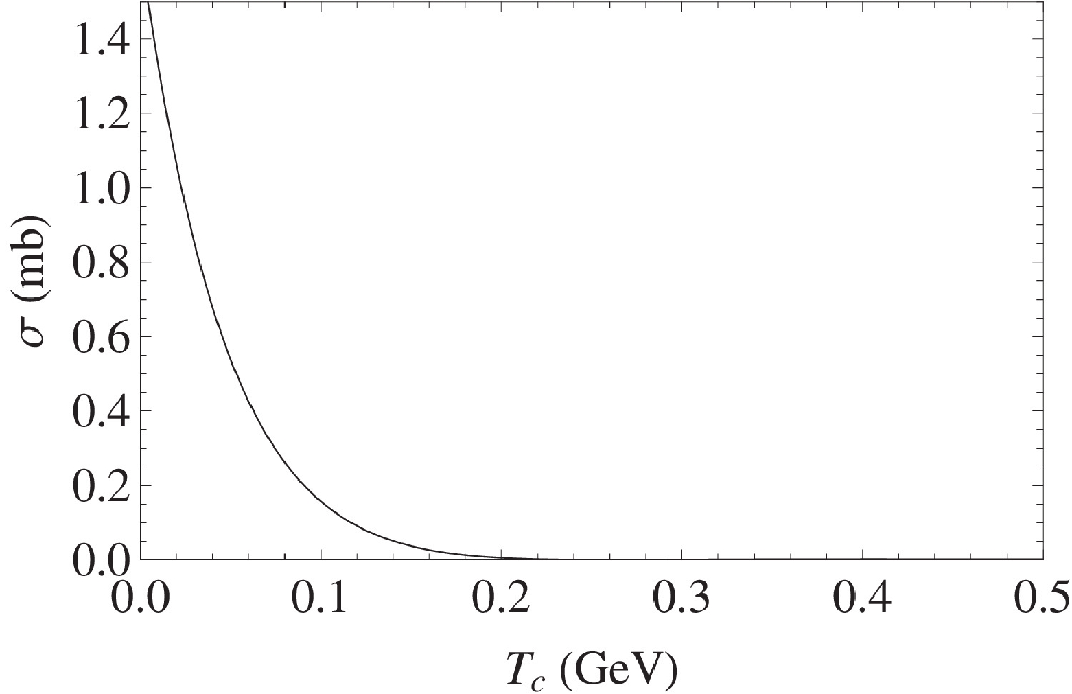
Figure 4. Total spin averaged cross sections versus Tc for quadratic potential.
-
After a discussion of the Cornell and quadratic potentials, we also incorporate Coulombic plus quadratic potential in our study. It is defined as
$ v_{ij} = Cr^{2}_{ij} - \frac{4}{3} \frac{\alpha_{s}}{r_{ij}} + \bar{C} , $

(26) where
$i,j = 1,2,\bar{3},\bar{4} .$ For Coulombic plus quadratic potential, the parameters
$ \alpha_{s} $ , C, and$ \bar{C} $ are adjusted by minimizing$ \chi^{2} $ between the masses taken from [42] and a spectrum generated by using the Coulombic plus quadratic potential in the quark potential model for the mesons$ \eta_{c} $ ,$ J/\psi $ ,$ h_{c} $ ,$ \chi_{c0} $ ,$ \chi_{c1} $ , and$ \chi_{c2} $ . The quark mass is taken from [46]. For the Coulombic plus quadratic potential, the values of the parameters are d$ = 1.00 $ GeV$ ^{-1} $ , constituent quark mass m = 1.93 GeV,$ M_{J/\psi} $ = 3.10 GeV,$ \alpha_{s} $ = 0.3, C = −0.047 GeV$ ^{3} $ , and$ \bar{C} $ = 0.792 GeV. The results are shown in Table 3.Total COM energy Tc /GeV Total cross section $\sigma$ /mb

0.01 0.282 0.02 0.269 0.03 0.244 0.04 0.222 0.1 0.121 0.2 0.0472 0.3 0.0173 0.4 0.00544 0.5 0.00121 Table 3. Total spin averaged cross sections versus selected values of Tc for Coulombic plus quadratic potential.
It is observed in Figure 5 that if we replace the linear confinement with the quadratic one in the Coulombic plus linear potential, the magnitudes of the cross sections lie in between the two, i.e., the quadratic and Cornell potentials. As noted in our earlier work [47], the meson sizes obtained via two potential models show a remarkable difference in magnitude, i.e., the meson size d calculated for the quadratic potential is approximately 1.5 times greater than its value for the Cornell potential. A possible explanation could take into account the respective shapes of the two potentials for any given value of energy E. Thus, for a specific energy E, the value of the classical turning point
$ r_{0} $ (E =$ V(r_{0}) $ ) is greater for the quadratic potential than the Cornell potential, and beyond the classical turning point (where E <$ V(r) $ ), the state-function dampens rapidly. This means that a greater value of the classical turning point for quadratic potential gives us a larger rms radius compared to the Cornell potential. The rms radii for the Cornell and quadratic potentials are d =$ 0.995 $ GeV$ ^{-1} $ and d = 1.49 GeV$ ^{-1} $ (where$ d = $ $ \sqrt{\frac{1}{2 \mu \omega}} $ [39]), respectively.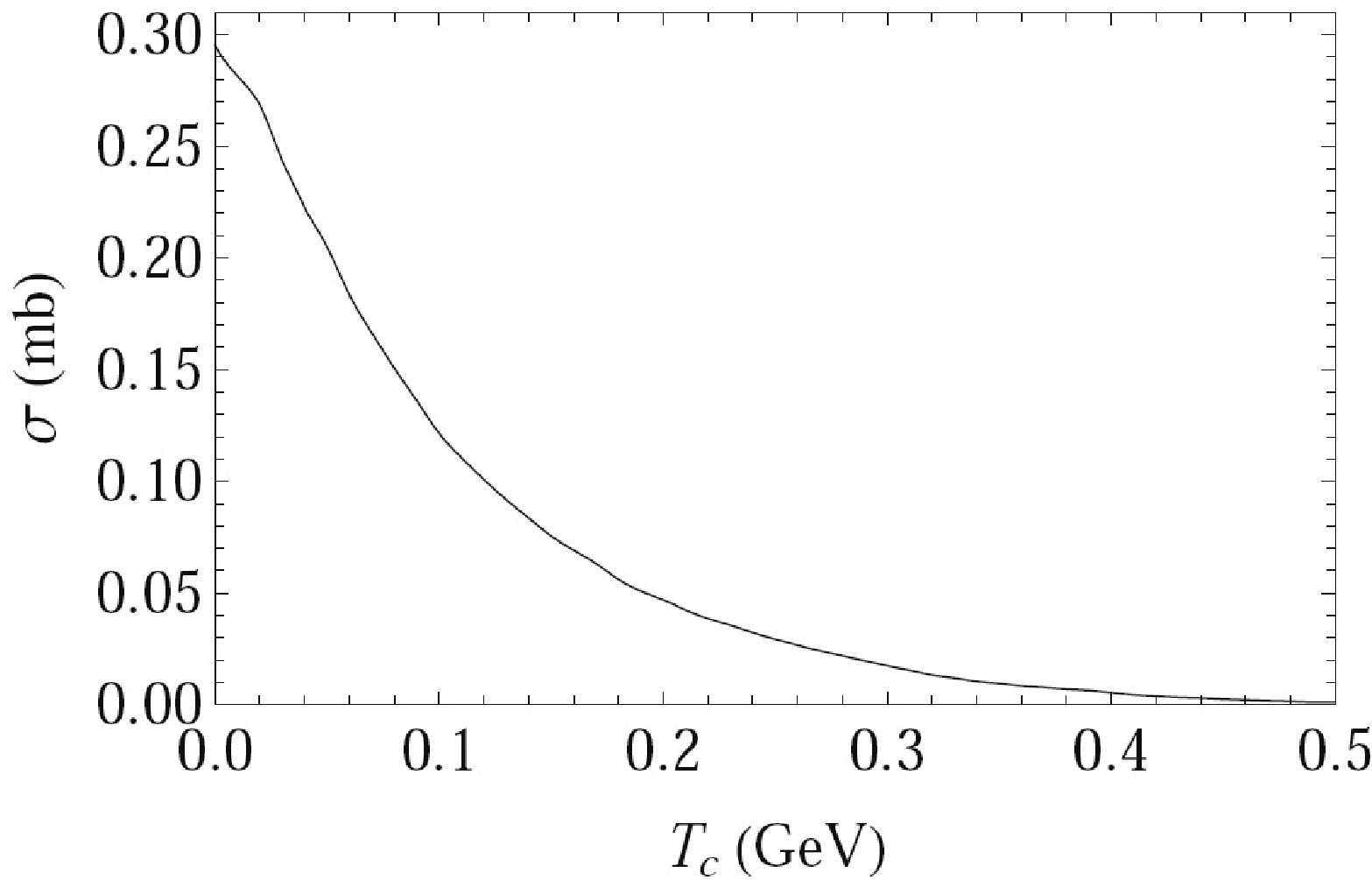
Figure 5. Total spin averaged cross sections versus Tc for Coulombic plus quadratic potential.
Lastly, we can also study the effect of scattering angles on the aforementioned cross sections for the quadratic potential. The results for different angles (such as
$ \varphi $ =$ 0^{\circ} $ ,$ 30^{\circ} $ ,$ 60^{\circ} $ ,$ 90^{\circ} $ ) between the two incoming waves can be plotted. However, it can be shown that varying the scattering angle has no effect whatsoever on the respective cross sections, i.e., the graphs for different values of scattering angle$ \varphi $ overlap if plotted simultaneously. Hence, the scattering cross sections are independent of the angles between the two incoming waves. -
We have considered
$ J/ \psi $ -$ J/\psi $ scattering using quadratic and Cornell potentials. The qualitative behavior of both graphs is identical, i.e., with an increase in total COM energy, the scattering cross sections gradually decrease. However, by using quadratic potential, we obtain higher magnitudes of scattering cross sections. It is pertinent to mention that, throughout our discussion, we have reported our model-dependent results up to three significant figures.At low energies, only S-wave scattering is significant. The contribution to scattering cross sections from other partial waves, with I
$ > $ 0, is negligible. As we are studying the case of S-waves, it can be seen that, as the energy increases, the scattering cross sections decrease, in accordance with the experimental results (lattice QCD simulations) for other scatterings. The quadratic confinement is a good approximation of the more realistic Cornell potential regarding the properties of conventional hadrons. However, this comparison shows that, for tetraquark systems, the quadratic confinement does not appear to be a good approximation of Cornell confinement. Therefore, to find the properties of four quark systems, such as the spectra of four quark states, it is recommended to not use the quadratic confinement as a replacement for the Cornell potential for future studies.As heavy quarkonia decay strongly, it is very difficult to directly measure the dissociation cross sections in hadron scattering experiments. As we mentioned in our introduction, the cross sections are calculated using theoretical approaches. One such theoretical approach, called the quark-interchange model [47], has been successfully supported with light hadron scattering data (I = 2
$ \pi\pi $ [31],$ I = 3/2 $ $ K\pi $ [48], and$ I = 0,1 $ $ K,N $ [49]). While we have retained the basic features of the quark-interchange model, our improvements to certain treatments in it suggest that our calculations may be reasonably sound regarding heavy hadron-hadron scattering. However, a direct comparison with experimental data on heavy hadron interaction is not possible. In future, it may be useful to verify our predicted cross sections using detailed Monte-Carlo simulations. If our findings are shown to be reasonably accurate, it will be clearly beneficial to include these insights in simulations involving hadron processes in heavy-ion collisions and other studies concerning tetraquark states.
J/ψ-J/ψ scattering cross sections of quadratic and Cornell potentials
- Received Date: 2020-06-17
- Accepted Date: 2020-09-22
- Available Online: 2021-02-15
Abstract: We study the scattering of


 DownLoad: