


 Abstract
 HTML
HTML Reference
 Related
 PDF
PDF


-
After assuming that the UV completion of the Standard Model Effective Field Theory (SMEFT) satisfies S-matrix and quantum field theory (QFT) axiomatic properties, such as Lorentz invariance, unitarity, analyticity, and locality, one can show that the SMEFT dimension-8 Wilson coefficients must satisfy the so-called positivity bounds [1-6] (see, e.g., Refs. [7-11] and the references therein for generic discussions). While these bounds could guide experimental searches for physics beyond the Standard Model (SM), one might, conversely, consider them to test the axiomatic principles of QFT experimentally [12]. If the measurements of the values of the Wilson coefficients violate the positivity bounds, the underlying UV model must violate at least one of those principles. Therefore, new ideas beyond conventional model building approaches are required.
Another interesting feature of the dimension-8 coefficient space is that, by exploiting its positive nature, we can either infer the existence of UV states and their quantum numbers [3] or exclude them. This originates from the positivity bounds that carve out a geometric object in the parameter space of the Wilson coefficients, namely a convex cone whose “edges” (to be more precisely defined later) are closely related to the properties of the UV states lying in specific irreducible representations (irreps) of the SM symmetry group. This relation, when combined with the positive nature of the dimension-8 coefficient space, can often provide striking information about the new physics states living in the UV.
As an extreme example, one could imagine that one succeeds in measuring the vector of dimension-8 Wilson coefficients with sufficient precision. If this vector coincides with one of the “edges” of the cone, the UV states generating the corresponding operators can be uniquely determined in the sense that they must all lie in a single irrep of the SM symmetries. If the UV completion is assumed to be tree-level and weakly coupled, one concludes that the underlying theory must be a “one-particle extension” of the SM. This provides an answer to the “inverse problem” [13-15] that can be summarized as follows. Given the measured values of the coefficients at the electroweak scale, how can we possibly determine the nature of the new physics beyond the SM? Similarly, if the measurement agrees with the SM value to a sufficient precision, one can simultaneously exclude the existence of any potential new physics state up to certain scales. This exclusion is guaranteed by the positive nature of the Wilson coefficients and cannot be removed by arranging the UV states in specific patterns that cancel each other's effects. Therefore, this would provide a model-independent confirmation of the SM, which is not possible when truncating the SMEFT at dimension-6.
Dimension-8 SMEFT operators [16, 17] have recently attracted increasing attention, in particular as the LHC accumulates more data. Various motivations for going beyond a truncation of the SMEFT Lagrangian at the dimension-6 level have correspondingly been presented, for example, in Refs. [4, 6, 18-24]. In addition, observables that can be used to disentangle the effects of dimension-8 operators from those of dimension-6 have been proposed and studied, as for example, in Refs. [25, 26]. However, positivity-related topics, including the possible tests of its violation and the option of inferring/excluding the existence of states in the UV, have not been discussed using realistic phenomenological examples.
This study aims to present some initial results in this direction in the context of future lepton colliders. In particular, we are interested in the following questions:
1. To what extent can we test any potential violation of the positivity bounds?
2. For realistic measurements (including the associated experimental errors), to what extent can we learn about the existence of UV states and their properties using the positive nature of the dimension-8 coefficient space?
The first point has been discussed in Ref. [12] but not in the SMEFT framework, and no realistic collider analysis has been presented. In contrast, the second point has not been discussed in literature.
Several proposals for a future electron-positron machine are currently discussed, including the CEPC [27], FCC-ee [28, 29], ILC [30, 31], and CLIC [32] projects. These colliders present an ideal means to perform high accuracy measurements, particularly as they are planned to be operated at various center-of-mass energies. Thus, they could allow us to distinguish the effects of dimension-8 operators from those of dimension-6 on a large set of observables, thus creating new opportunities to access to information on the SMEFT dimension-8 operators. Let us note that in addition to the energy dependence, the angular momentum can also be used as a discriminant [25].
For a first step in this direction, we consider the simplest
$ 2\to 2 $ process that could occur at a lepton collider and that is expected to be one of the most accurately probed processes,$ e^+e^-\to e^+e^- $ , and investigate the impact of the SMEFT four-fermion operators. We ignore other$ e^+e^-\to ff $ channels with other final-state fermion species, as the corresponding positivity bounds involve not only$ e^2f^2 $ operators but also$ e^4 $ and$ f^4 $ operators. On the contrary,$ e^+e^-\to e^+e^- $ is self-contained in the sense that only$ e^4 $ operators are relevant, and their positivity bounds do not involve other operators at leading order. A more comprehensive study including more operators and processes can be undertaken, but we leave it for the future.The remainder of this paper is organized as follows. In Section II, we list the
$ e^4 $ dimension-6 and dimension-8 operators relevant to our study. In Section III, we derive the positivity bounds on these operators by using the elastic scattering of arbitrarily superposed states. We propose a variable to quantify the amount of potential positivity violation in Section III.1 to connect the collider reaches with the underlying physics and discuss its possible interpretations in Section III.2. Then, in Section IV, we briefly discuss how to infer/exclude the existence of UV states using dimension-8 positivity. Subsequently, in Section V, we study the phenomenological aspects of positivity for several$ e^+e^- $ collider scenarios. Finally, we summarize our main findings in Section VI. -
The SMEFT Lagrangian is generically defined as
$ {\cal L}_{\rm{SMEFT}} = {\cal L}_{\rm{SM}}+\sum\limits_i\frac{C_i^{(6)}}{\Lambda^2}O_i +\sum\limits_i\frac{C_i^{(8)}}{\Lambda^4}O_i+\cdots\ , $

(1) where the
$ C_i $ parameters represent the various Wilson coefficients associated with the higher-dimensional operators$ O_i $ , and$ \Lambda $ denotes the cutoff scale of the theory. At the tree level, two classes of effective operators are relevant for$ e^+e^- \to e^+e^- $ scattering. The first one involves four electron fields (four-fermion operators), and the second one involves two electron fields (e.g., the operators affecting the$ \bar eeZ $ or$ \bar ee\gamma $ vertices) or fewer (e.g., the operators modifying the electroweak boson two-point functions). For a feasibility study, we solely focus in this work on four-fermion operators, assuming that the other potentially relevant operators can be determined or constrained by the study of other$ e^+e^-\to X $ channels. We also ignore any possible loop-level correction within the SMEFT framework.There are three four-fermion
$ e^4 $ operators that arise at dimension-6 [33],$ \begin{aligned}[b] O_{ee} = &( \bar e \gamma^\mu e )\ ( \bar e \gamma_\mu e)\ ,\\ O_{el} =& ( \bar e \gamma^\mu e )\ ( \bar l \gamma_\mu l)\ ,\\ O_{ll} =& ( \bar l \gamma^\mu l )\ ( \bar l \gamma_\mu l)\ , \end{aligned} $

(2) and all of which provide independent contributions to
$ e^+e^-\to e^+e^- $ scattering. We use the notations$ C_{ee} $ ,$ C_{el} $ , and$ C_{ll} $ below to denote their dimensionless Wilson coefficients.The full basis of dimension-8 operators has been presented recently [16, 17]. Three types of four-electron operators are relevant to our study and are of the forms
$ \Psi^4D^2 $ (four-fermion operators including two derivatives),$ \Psi^4H^2 $ (four-fermion operators including two extra Higgs fields), and$ \Psi^4DH $ (four-fermion operators including one derivative and one extra Higgs field).In this study, we are mainly interested in operators
$ \Psi^4D^2 $ of the first category, as they are subject to positivity bounds. There are five such independent operators for which we choose the following basis:$ \begin{aligned}[b] &O_{1} = \partial^\alpha(\bar e \gamma^\mu e) \partial_\alpha (\bar e \gamma_\mu e)\ ,\\ &O_{2} = \partial^\alpha(\bar e \gamma^\mu e) \partial_\alpha (\bar l \gamma_\mu l)\ ,\\ &O_{3} = D^\alpha(\bar e l)\ D_\alpha(\bar l e), \\ &O_{4} = \partial^\alpha(\bar l \gamma^\mu l)\ \partial_\alpha(\bar l \gamma_\mu l)\ ,\\ &O_{5} = D^\alpha(\bar l \gamma^\mu \tau^I l)\ D_\alpha(\bar l \gamma_\mu \tau^I l)\ , \end{aligned} $

(3) where the
$ \tau^I $ matrices are the Pauli matrices. The operators$ O_{4} $ and$ O_{5} $ contribute identically to$ e^+e^-\to e^+e^- $ ; therefore, this process is only sensitive to the four independent coefficient combinations$ C_1 $ ,$ C_2 $ , C3, and$ C_4+C_5 $ , where$ C_i $ denotes the Wilson coefficient associated with the operator$ O_i $ . Consequently, in the collider discussions below, we will always set$ C_5 = 0 $ . This is equivalent to restricting our discussion to four independent degrees of freedom in the considered process, ignoring the fact that the left-handed electron and neutrino live in the same$ SU(2)_L $ doublet.Similar to a model-independent SMEFT framework, the other two classes of dimension-8 operators should be included as well. However, in the context of
$ e^+e^-\to e^+e^- $ scattering, the$ \Psi^4H^2 $ operators act like dimension-6 operators (after replacing the two Higgs fields by their vacuum expectation value). Thus, these operators can only be disentangled from those of dimension-6 when more observables are included, such as those related to neutrino DIS experiments. In our study, these operators can be fully captured by shifting the three dimension-6 coefficients of Eq. (2). Once the latter are marginalized over, they have no impact on the determination of the dimension-8 operators of the first category$ \Psi^4D^2 $ . Finally, the$ \Psi^4DH $ operators can be omitted by assuming a$ U(3)^5 $ flavor symmetry.In summary, our collider analysis only incorporates the effects of the dimension-8 operators of the first type
$ \Psi^4D^2 $ . In what follows, we frequently refer to a vector notation for the Wilson coefficients,$\begin{aligned}[b] \vec C^{(6)} = (C_{ee},C_{el},C_{ll}), \quad \vec C^{(8)} = (C_1,C_2,C_3,C_4)\ .\end{aligned}$

(4) This allows for a parameterization of (differential) cross sections up to
$ {\cal O}(\Lambda^{-4}) $ as$ \sigma = \sigma_{\rm{SM}} +\! \sum\limits_i\frac{C_i^{(6)}}{\Lambda^2}\sigma^{(6)}_i \!+\!\sum\limits_i\frac{[C_i^{(6)}]^2}{\Lambda^4}\sigma^{(6)}_{ii} \!+\!\sum\limits_i\frac{C_i^{(8)}}{\Lambda^4}\sigma^{(8)}_i \ , $

(5) where
$ C_i^{(6)} $ and$ C_i^{(8)} $ run through all the components of the vectors$ \vec C^{(6)} $ and$ \vec C^{(8)} $ . This expression includes the fact that, in the (adopted) limit of$ m_e\to0 $ , there is no interference between two different dimension-6 operators. We have computed the different$ \sigma $ terms both analytically and by using FeynRules [34] to generate a UFO library [35] to be used within MadGraph5_aMC@NLO [36]. To assess the impact of truncating the$ 1/\Lambda $ expansion, we also include the next order terms in some of our results. Equivalently, we add interference terms involving a$ C^{(6)}_i C^{(8)}_j $ product and the quadratic contributions in the$ C^{(8)}_i $ coefficients. -
Positivity bounds can be derived from a dispersion relation and the optical theorem, which are based on fundamental QFT principles including unitarity, analyticity, locality, and Lorentz invariance. This is a very active field with a vast and growing literature, and in this regard, we refer to Refs. [7-10] and the references therein and to Refs. [1-6] for specific SMEFT applications.
The conventional approach to derive positivity bounds utilizes forward and elastic scattering amplitudes (see, e.g., Ref. [1]). Briefly, it requires that the second order s-derivative of the elastic amplitudes (with poles subtracted) be positive. For instance, for the process considered in this study, it is given by
$ \frac{ {\rm{d}}^2}{ {\rm{d}} s^2}M(e^+e^-\to e^+e^-)\geqslant 0 . $

(6) The l.h.s. of this equation consists of a linear combination of the considered
$ \Psi^4D^2 $ operator coefficients, and the above requirement determines the sign of this combination. More specifically, different bounds can be derived by choosing different fermion species and chiralities, as for example with●
$ M(e_R e_R\to e_R e_R) $ :$ C_1\leqslant 0 $ ;●
$ M(e_L e_L\to e_L e_L) $ :$ C_4+C_5\leqslant 0 $ ;●
$ M(e_R \bar e_L\to e_R \bar e_L) $ :$ C_3\geqslant 0 $ ;●
$ M(e_L \nu_L\to e_L \nu_L) $ :$ C_5\leqslant 0 $ .However, the above list of bounds is not complete, as, by defining states through the superposition of different flavors and chiralities, one can consider extra elastic scattering processes [37]. According to this approach, the best bounds are derived in Appendix A from the scattering amplitudes presented in Appendix B,
$ C_1\leqslant 0 , $

(7) $ C_4+C_5\leqslant 0, $

(8) $ C_5\leqslant 0, $

(9) $ C_3\geqslant 0, $

(10) $ 2\sqrt{C_1(C_4+C_5)}\geqslant C_2, $

(11) $2\sqrt{C_1(C_4+C_5)}\geqslant-(C_2+C_3). $

(12) While the first four bounds are obtained without considering any superposition, those in Eqs. (12) and (13) arise from the superpositions
$ \begin{aligned}[b] | f_\pm \rangle \equiv &\frac{(C_4+C_5)^{1/4}} {\left[(C_4+C_5)^{1/2}+C_1^{1/2}\right]^{1/2}} | e_R\rangle \\& \pm \frac{C_1^{1/4}} {\left[(C_4+C_5)^{1/2}+C_1^{1/2}\right]^{1/2}} |\bar e_L\rangle , \end{aligned} $

(13) and the scattering processes
$ f_\pm f_\mp \to f_\pm f_\mp $ and$f_\pm f_\pm \to $ $ f_\pm f_\pm $ , respectively. Moreover, these two bounds are homogenous and written as quadratic inequalities of the Wilson coefficients.The above approach is sufficient for the study of the four-fermion operators considered in this paper. However, in general, it is insufficient to obtain the best possible bounds. Accordingly, a new and better approach has been proposed recently [3]. The idea is to construct the allowed Wilson coefficient parameter space region directly as a convex cone, which is a convex hull of its extremal rays, and the latter can be identified using group theoretical considerations.
This new approach has at least two advantages. First, it always provides the tightest constraints available from the dispersion relation. They may be tighter than those that can be obtained by relying on the conventional elastic positivity approach, as for example, for the scattering of a pair of W-bosons. Second, more relevant to this study (see Section IV), it reveals a connection between the positivity bounds and the existence of new physics states in the UV. In order for this connection to be manifest, one needs to determine the exact shape of the parameter space allowed by the bounds, which cannot always be achieved with the conventional approach for complicated cases. We have verified that, for the operators under consideration, the two methods yield the same set of bounds of Eqs. (7)–(12).
We devote the remainder of this section to a discussion on the possible violation of positivity and its physical implications.
-
A positivity violation would imply a breakdown of the fundamental principles of QFT. Hence, if such a violation is observed at a future collider, it would be mandatory to study the physics behind it. To this end, we first need a model-independent way to quantify the observed amount of violation, which can be connected later to possible physics scenarios.
The physical quantity to consider for probing a potential positivity violation is the second order s-derivative of the studied amplitude with poles subtracted,
$ M(s, t = 0) $ . Introducing the explicit dependence on the fermion mixing parameters$ \epsilon_i = (a_i,b_i,c_i) $ of Eq. (64), we can define$ -\Delta^{-4}\equiv \min\left[ \min\limits_{\epsilon_1,\epsilon_2} \frac{1}{2} \frac{ {\rm{d}}^2M(s,t = 0)(\epsilon_1,\epsilon_2)}{ {\rm{d}} s^2},0\right]\ , $

(14) so that
$ \Delta $ has a mass dimension 1 and indicates the maximal amount of positivity violation reached when the$ \epsilon_i $ mixing parameters vary. Thus, if positivity is always satisfied,$ \Delta = \infty $ . For the amplitude to be physical, we impose the constraints$ |\epsilon_{1,2}| = 1 $ . Generically, there will be several contributing operators, so that it is convenient to consider the level of the amplitude directly instead of that of the Wilson coefficients. Ultimately, the amplitude contains the essential physical information of the theory, whereas the operators in the Lagrangian are subject to ambiguities originating from field redefinitions.While the physical interpretation of the
$ \Delta $ quantity will be discussed in Section III.2, we briefly comment below on its relation with the scale of new physics$ \Lambda_{\rm{BSM}} $ . Let us assume that a set of Wilson coefficients is measured, and both$ \Lambda_{\rm{BSM}} $ and$ \Delta $ can be estimated/computed from these coefficients. Intuitively, we expect the scale$ \Delta $ to be larger, as a deviation from the SM does not necessarily imply positivity violation. On the contrary, the latter implies that beyond the SM (BSM) physics must exist.One often estimates
$ \Lambda_{\rm{BSM}} = \Lambda/\sqrt[4]{C} $ , where C represents a typical dimension-8 Wilson coefficient. However, if multiple coefficients are nonzero, it is instead more natural to infer$ \Lambda_{\rm{BSM}} $ from the amplitude that is physical and basis-independent. It is desirable to use the largest possible amplitude obtained when varying the initial-state and final-state superpositions,$ \Lambda_{\rm{BSM}}^{-4} = \max\limits_{\epsilon_1,\epsilon_2}\left| \frac{1}{2}\frac{ {\rm{d}}^2M(s,t = 0)(\epsilon_1,\epsilon_2)}{ {\rm{d}} s^2}\right|\ , $

(15) where the second-order derivative allows for the extraction of the dimension-8 deviations from the SM. Hence,
$ \Lambda_{\rm{BSM}}\lesssim\Delta $ is as intuitively expected.To compute the positivity violation measure
$ \Delta $ , a simple option is to find the set of$ \epsilon_i $ mixing parameters that saturates to the bounds of Eqs. (7)–(12). These bounds can be considered as the supporting planes of a convex cone representing the set of points in the Wilson coefficient parameter space that can be UV-completed [3]. Thus, for any point located outside the cone,$ \dfrac{1}{2}\dfrac{ {\rm{d}}^2M}{ {\rm{d}} s^2} $ is related to the distance to any supporting plane of the cone (or in other words, the$ \Delta $ parameter). This yields$ \Delta^{-4} = \frac{\delta(\vec C^{8})}{\Lambda^4}\ , $

(16) with
$ \begin{aligned}[b] \delta(\vec C^{(8)})\equiv & -\min\bigg[0, -4C_1,-4(C_4\!+\!C_5),C_3,-8C_5, \\ & \Theta[C_2 \!-\!2\max(C_1,C_4\!+\!C_5)] \frac{C_2^2\!-\!4C_1(C_4\!+\!C_5)}{C_1\!-\!C_2\!+\!C_4\!+\!C_5},\\ & \Theta[-C_2-C_3-2\max(C_1,C_4+C_5)]\\ & \times\frac{(C_2+C_3)^2-4C_1(C_4+C_5)}{C_1+C_2+C_3+C_4+C_5}\bigg] , \end{aligned} $

(17) where
$ \Theta[x] $ is the standard Heaviside function. One can then use either$ \Delta^{-1} $ or$ \delta(\vec C^{(8)}) $ to assess the amount of positivity violation. The former is dimensionful and directly connected to the scale at which the fundamental QFT principles are violated, whereas the latter is dimensionless and intended to be combined with$ \Lambda^{-4} $ .However, it is not necessarily sufficient to derive the
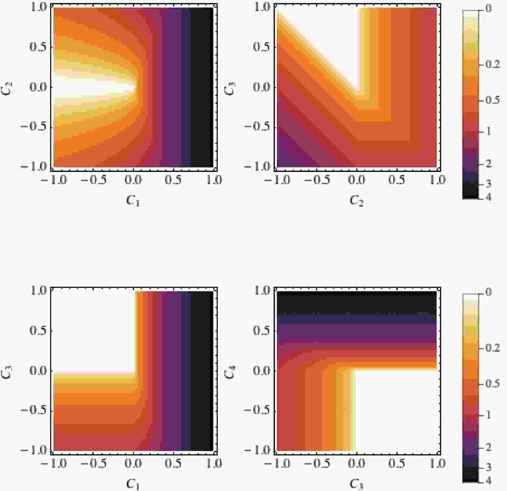
$ \epsilon_i $ values yielding the six bounds of Eqs. (7)–(12). A priori, there might exist a supporting plane that provides a larger amount of positivity violation, although as a positivity bound, it can be positively decomposed into a combination of Eqs. (7)–(12). Therefore, it is redundant and discarded. The rigorous way to estimate$ \Delta $ is to rely on the definition of Eq. (14) and minimize its right-hand side. We have numerically checked that, for more than 90% of the parameter space, the difference between the exact method and the approximation of Eq. (17) is less than 10%. Therefore, we consider the latter as a convenient estimate.As an illustration, Fig. 1 shows the dependence of the quantity
$ \delta(\vec C^{(8)}) $ on the different considered Wilson coefficients. We focus on several two-dimensional slices of the parameter space that we define by setting the irrelevant coefficients$ C_i $ to 0. Thus, the white areas for which$ \delta(\vec C^{(8)}) = 0 $ satisfy positivity. We can observe that the amount of violation increases as one moves further away from the positive regime.
Figure 1. (color online) Amount of positivity violation in the studied dimension-8 Wilson coefficient parameter space. We consider several two-dimensional slices of the parameter space that we define by setting all Wilson coefficients but two to 0. Positivity violation is estimated through the quantity
$\delta(\vec C^{(8)})$ of Eq. (17), so that the white areas correspond to regions compliant with positivity. -
What do possible violations of positivity bounds mean? It is known that the forward positivity bounds are derived by assuming that the scattering amplitudes computed in the UV-completed theory are unitary, Lorentz invariant, polynomially bounded in momenta and analytical in the complex s plane, apart from certain poles and branch cuts. The unitarity of the S-matrix indicates that the quantum mechanical probabilities of all possible scatterings add up to 1, which results in the optical theorem, or that the imaginary part of the UV amplitudes is positive in the physical region.
Violations of unitarity, such as the existence of (bad) ghosts [38] in the UV, will lead to catastrophic instabilities in the theory (and thus should be avoided), unless the ghosts only appear in the effective field theory context and with a mass at or greater than the cutoff scale. Lorentz invariance has been tested at very high energy scales via various experiments, although certain properties are only weakly constrained [39]. Analyticity is implied by causality and can be proven to be valid at any perturbative order, although it has never been proven non-perturbatively. The polynomial boundedness of the amplitudes in the momentum space originates from locality, the lack of which would result in ill-defined Fourier transforms and non-locality in real space. In addition, polynomial boundedness, analyticity, and unitarity can be used to prove the Froissart bound that implies that forward UV amplitudes should grow slower than
$ s\ln^2 s $ when$ s\to \infty $ [40]. This allows for the derivation of the dispersion relation (another important element to derive the positivity bounds).In terms of the Wilson coefficient parameter space, the observation of small violations of the positivity bounds would indicate regions not too far away from the positive regime (e.g., the yellow/orange areas in Fig. 1) and would imply that some of the fundamental principles of QFT are violated at certain energy scales. A high experimental precision is required to detect those small violations. In contrast, the observation of a stronger violation of the positivity bounds would indicate regions further away from the positive regime (e.g., the purple/black areas in Fig. 1) and imply violations of the fundamental principles of QFT at more accessible energies.
On dimensional grounds, the quantity
$ \Delta $ introduced in Section III.1 regulates the amount of positivity violation. However, how well does$ \Delta $ connect to the actual positivity violation scale? To investigate this issue, we consider a scenario in which the fundamental principles of QFT are violated at some energy scale$ \Lambda_* $ . In this case, we can only push the dispersion relation up to the scale$ \Lambda_* $ in the complex s plane, rather than to infinity where the semi-circular contour integrations vanish by virtue of the Froissart bound (see, e.g., Ref. [2]). Such an earlier cutoff could be due, for instance, to some new singularities at$ |s| = \Lambda_* $ lying away from the real axis. If we additionally assume that$ \Lambda_* $ is parametrically greater than the mass scale$ M_{\rm{BSM}} $ of new particles living in the UV, the dispersion relation can be written as$ \begin{aligned}[b] \frac12 \frac{ {\rm{d}}^2 M(s = 2m_e^2,t = 0)}{ {\rm{d}} s^2} =& \int^{\Lambda_*^2}_{4m_e^2} \frac{ {\rm{d}} s'}{2\pi} \frac{\Im[M(s',0)]}{(s'-2m_e^2)^3} \\& + \int_{{\cal C}'}\frac{ {\rm{d}} s'}{2\pi i} \frac{M(s',0)}{(s'-2m_e^2)^3} , \end{aligned} $

(18) where
$ {\cal C}' $ denotes the two semi-circular contours at$ |s| = \Lambda_* $ . The integral around the branch cuts along the real axis is positive by the usual argument of positivity bounds, so that the violation of positivity could be estimated by evaluating the integral along the$ {\cal C}' $ contour.To estimate the integrand at
$ |s| = \Lambda_* $ , we focus on simple tree-level UV-completions in which the$ e^+e^-\to e^+e^- $ scattering is mediated by the exchange of a heavy scalar or vector boson coupling with a strength$ g_{\rm{BSM}} \simeq 1 $ . This leads to two distinct cases.1.
$ M(s',0) \sim g^2_{\rm{BSM}}\dfrac{s'}{s'-M^2_{\rm{BSM}}} $ , which corresponds to an s-channel scalar or vector exchange. This yields the violation$ \int_{{\cal C}'}\frac{ {\rm{d}} s'}{2\pi i} \frac{M(s',0)}{(s'-2m_e^2)^3} \simeq \frac{1}{\Lambda_*^4}\ . $

(19) 2.
$ M(s',0) \sim {s' g^2_{\rm{BSM}}}/{M_{\rm{BSM}}^2} = s'/\Lambda_{\rm{BSM}}^2 $ , which corresponds to a t-channel scalar or vector exchange. This yields the violation$ \int_{{\cal C}'}\frac{ {\rm{d}} s'}{2\pi i} \frac{M(s',0)}{(s'-2m_e^2)^3} \simeq \frac{1}{\Lambda_*^2 \Lambda_{\rm{BSM}}^2}\ . $

(20) We should emphasize that these simple scenarios do not lead to any positivity violation. We are solely using them as rough estimates for the potential size of the boundary term in Eq. (18), assuming that the Froissart bound approximately holds below
$ \Lambda_* $ . This shows that, in the first case, we can use$ \Delta $ as an estimate of the scale$ \Lambda_* $ at which the fundamental principles of QFT are violated. In contrast, in the second case,$ \Delta = \sqrt{\Lambda_{\rm{BSM}}\Lambda_*} $ . As we have argued that$ \Delta>\Lambda_{\rm{BSM}} $ (see Section III.1),$ \Delta $ is thus lower than the actual scale$ \Lambda_* $ . As both$ \Delta $ and$ \Lambda_{\rm{BSM}} $ can be inferred from a measurement, one can estimate$ \Lambda_* $ as$ \Delta^2/\Lambda_{\rm{BSM}} $ .The fact that
$ \Lambda_* $ is either around (first scenario) or above (second scenario)$ \Delta $ is consistent with the assertion of Ref. [12]. However, any further determination beyond this rough estimation is difficult without an apparent characterization of the BSM nature. But what are the possible scenarios in which positivity may be violated? There are several possibilities that will be (incompletely) enumerated in the following.First, for the UV completions of the SM that are intertwined with the massless graviton, the
$ e^+e^-\to e^+e^- $ scattering amplitude contains a t-channel pole with an$ s^2 $ dependence, and it blows up in the forward limit (see e.g. Ref. [41]). Therefore, the usual twice-subtracted dispersion relation and the second-order s-derivative bound of Eq. (6) cannot be directly used. It is observed that the standard positivity bounds, which merely require the subtraction of the infinite t-channel pole, can be violated, as shown in some explicit examples in Refs. [42, 43] (see also the work of Ref. [41] for the opposite argument). This violation is conjectured to be suppressed by the quantum gravity scale, which is usually the Planck scale, although it could be much lower. For example, in ADD models [44, 45] with two extra dimensions, the fundamental scale for gravity is around the TeV scale.If one assumes that the UV theory follows the Regge behavior,
$ \Im[M(s\to \infty, t\to 0)] = f(t)\left(\frac{\alpha^{\prime} s}{4}\right)^{2+j(t)}, $

(21) where
$ \alpha' = M_s^{-2} $ is the “string scale” of gravity, one can exactly quantify positivity violation [46],$ \begin{aligned}[b] \frac{ {\rm{d}}^2 M}{ {\rm{d}}^2 s}>& -\frac{f \alpha^{\prime 2}}{4 \pi}\left[\frac{f^{\prime}}{f j^{\prime}}+\ln \left(\frac{\alpha^{\prime} M_{*}^{2}}{4}\right)\right]\\ & +\frac{f \alpha^{\prime 2}}{4 \pi}\left[\frac{j^{\prime \prime}}{2\left(j^{\prime}\right)^{2}}+O\left(\frac{1}{\alpha^{\prime} M_{*}^{2}}\right)\right] . \end{aligned} $

(22) In this expression, the primed quantities refer to a derivative with respect to t, evaluated at
$ t = 0 $ , and$ M_* $ represents the scale at which the Regge behavior is first observed. In this sense, a test of positivity violation would allow us to probe the quantum gravity scale and study the implications of low scale gravity.Second, one could devise a simple example demonstrating how unitarity violation leads to positivity violation in the Effective Field Theory (EFT). One such popular model having an interesting bearing for inflation consists of the so-called DBI model [47], whose effective Lagrangian is given by
$ {\cal L}_{\rm EFT} = \varepsilon \Lambda^{4}-\varepsilon \Lambda^{4} \sqrt{1-\frac{\varepsilon(\partial \phi)^{2}}{2\Lambda^{4}} } , $

(23) with
$ \varepsilon = 1 $ . Expanding around$ ( \partial\phi)^2 = 0 $ , the leading interaction term is given by$ \varepsilon ( \partial\phi)^4/(32\Lambda^4) $ , and the corresponding forward positivity bound is satisfied. In contrast, if we choose instead$ \varepsilon = -1 $ in Eq. (23), we obtain the so-called anti-DBI model [48] that features positivity violations. To view this from a UV perspective, we recall that the DBI and anti-DBI models can be derived from a two-field (partial) UV theory [49], whose Lagrangian is given by$ {\cal L}_{\rm{pUV}} = \frac{ ( \partial \chi)^2}{2} + \frac{\varepsilon e^{\frac{\chi}{M}}( \partial \phi)^2}2 - \Lambda^4\left(\cosh \frac{\chi}{M}-1\right) ,$

(24) where
$ \varepsilon $ ,$ \Lambda $ , and M are constants. At low energies, the heavy field$ \chi $ is frozen. Neglecting its kinetic term and integrating it out semi-classically, we obtain the Lagrangian of Eq. (23). From the Lagrangian of Eq. (24), we observe that the$ \phi $ field is a ghost (with$ \varepsilon = -1 $ ). Alternatively, we can choose$ \epsilon = 1 $ and send$ \Lambda^4 $ to$ -\Lambda^4 $ in Eq. (24), which again leads to the anti-DBI model. In this case,$ \phi $ is not a ghost, but now$ \chi $ is a tachyon [50], and the potential is unbounded from below. As ghosts or runaway potentials lead to some of the worst instabilities in QFT [38], positivity violations originating from this type of UV pathologies appear unlikely.Then, which of these QFT axiomatic principles is the weakest link? Arguably, it might be the polynomial boundedness/locality. Indeed, it is widely believed that gravity is non-local, and the UV completions of general relativity, such as string theories, violate polynomial boundedness [51]. This is intimately linked to the observation that black holes are formed in high-energy scatterings with gravity included, and their horizon radius increases with the scattering energy. Moreover, there are no local gauge invariant observables in gravity.
When contemplating UV completions for the SMEFT, one may consider that general relativity is also an EFT that needs to be UV completed and which might a priori be interconnected to the UV theory of the SMEFT. Hence, the SM and gravity may be (partially) UV completed together, potentially at an energy scale such as the TeV scale as in models with large extra dimensions. However, polynomial boundedness is also violated in some innocent looking (Minkowski space) field theories derived by taking certain low-energy limits of gravitational theories. For example, the galileon theory consists of a scalar EFT whose Lagrangian is given by
$ {\cal L} = \frac12 \partial^\mu\pi \partial_\mu \pi + \frac{ {\alpha}}{\Lambda^3} \partial^\mu\pi \partial_\mu \pi \partial^\rho \partial_\rho \pi + \cdots\ . $

(25) This Lagrangian possesses a generalized shift symmetry when the galileon field
$ \pi \to \pi+c+b^\mu x^\mu $ , with c and$ b_\mu $ being constants [52]. Such a setup arises in the decoupling limit of either the DGP braneworld model [53] or dRGT massive gravity [54]. As the$ ( \partial^\mu\pi \partial_\mu \pi)^2 $ term is forbidden by the generalized shift symmetry, the 2-to-2 scattering amplitude of this theory does not contain any$ s^2 $ term, so that the forward positivity bound is automatically violated.Discussions on positivity bounds and their implications have recently restarted in the context of the galileon theory [7]. As the violation is marginal, adding a softly-breaking mass term for the galileon allows one to satisfy the forward positivity bounds [8, 11, 55, 56]. Moreover, at least in some parameter space region, generalized, t-derivative, positivity bounds [9, 57, 58] are fulfilled. However, further generalized positivity bounds exclude the entire parameter space [59].
An important feature of the galileon theory along with the DGP model and the dRGT model is that they embed the so-called Vainshtein mechanism (see Ref. [51] and the references therein). It has been argued that theories including the Vainshtein mechanism should not have standard UV completions whose low-energy EFT satisfies the positivity bounds. Instead, the high-energy behavior is characterized by a phenomenon called classicalization, where semi-classical contributions dominate [51, 60] (see ref. [61] for discussions on classicalization in the anti-DBI model). Examples of those non-standard UV completions also appear in gauge theories, in the context of chiral perturbation theories [62].
Lorentz invariance is also at risk of being violated at high energies. After all, our intuition of Lorentz invariance comes from low energy and weak gravity environments. In general relativity, Lorentz invariance still holds in local inertial frames, but this may just be a prejudice. Hence, Lorentz violating models are widely discussed in several contexts [63], including Horava-Lifshitz gravity [64]. In this case, gravity is Lorentz violating in the UV, so that the theory is potentially renormalizable and flows to Lorentz-invariant general relativity at low energies (so that it may be relevant for collider physics).
Finally, one last possibility that could justify a positive
$ \Delta $ quantity may be the existence of new states at or not too far above the TeV scale, making the SMEFT framework invalid. Naively, in such cases, one expects to either directly produce the new states or observe large deviations in various channels. Depending on the UV model, it might still be possible that this “positivity violation” is a first indication that BSM physics exists at low scales, invalidating the SMEFT framework.In this study, we take an agnostic approach, leaving all these possibilities open, and, as a first step, focus on the phenomenological feasibility of probing positivity violation effects. If
$ \Delta>0 $ can be verified experimentally, it implies that either at least one of the fundamental principles is violated at the TeV scale or not too far above (so that unconventional new physics is required, as shown above in this subsection), or that the SMEFT is invalid (which is also a useful guidance). In the first case, the logical follow-up requires exploring specific scenarios under which the violation occurs by using the scale$ \Delta $ as an instructive handle connected to$ \Lambda_* $ . The precise pin-down of this violation scale in connection with specific UV models is nevertheless left for future works. -
The possibility of inferring the existence of new physics states in the UV by virtue of the positive nature of the dimension-8 Wilson coefficient parameter space has been recently demonstrated [3]. It relies on convex geometry, and some of its basic concepts are listed below.
● A convex cone (or cone) is a subset of a vector space that is closed under additions and positive scalar multiplications. A salient cone is a cone that contains no straight line. Thus, if
$ {\cal{C}} $ is salient, having both$ x\in {\cal{C}} $ and$ -x\in {\cal{C}} $ implies$ x = 0 $ .● An extremal ray of a convex cone
$ {\cal{C}}_0 $ is an element$ x \in {\cal{C}}_0 $ that is not a sum of two other elements in$ {\cal{C}}_0 $ . If we can write an extremal ray as$ x = y_1+y_2 $ with$ y_1,y_2\in {\cal{C}}_0 $ , we must have$ x = \lambda y_1 $ or$ x = \lambda y_2 $ ,$ \lambda $ being a real constant. For example, the extremal rays of a polyhedral cone are its edges.● The convex hull of a given set
$ {\cal{X}} $ is the ensemble of all convex combinations of points in$ {\cal{X}} $ , where a convex combination is defined as a linear combination of points where all the combination coefficients are non-negative and add up to 1.● The conical hull of a given set
$ {\cal{X}} $ is the ensemble of all positive linear combinations of elements in$ {\cal{X}} $ , denoted by cone($ {\cal{X}} $ ). The extremal rays of cone($ {\cal{X}} $ ) are a subset of$ {\cal{X}} $ .● The Krein-Milman theorem [65] states that a salient cone
$ {\cal{C}} $ is the convex hull of its extremal rays.We now begin with the second-order s-derivative of the forward elastic scattering
$ ij\to kl $ , which we denote by$ M^{ijkl} $ and is related to the UV amplitude via the dispersion relation [3]$ M^{ijkl} = \int_{(\epsilon\Lambda)^2}^{\infty} {\rm{d}}\mu {\sum\limits_{Z\;{\rm{ in }}\;{\bf{r}}}}' \frac{|\left\langle {{{Z}|{\cal M}|{\bf{r}}} |^2} \right\rangle } {\pi\left( \mu-\frac{1}{2}M^2 \right)^3} P_ {\bf r}^{i(j|k|l)}. $

(26) As more extensively detailed in Ref. [3],
$ \sum' $ denotes a summation over all possible intermediate$ Z\in {\bf r} $ states along with their phase space, and$ {\bf r} $ runs through all irreps of the$ SO(2) $ rotations around the forward scattering axis and the gauge symmetries of the SM. Moreover,$ P_ {\bf r}^{ijkl}\equiv \sum_\alpha C^{ {\bf r},\alpha}_{i,j}(C^{ {\bf r},\alpha}_{k,l})^* $ represents the projective operators of$ {\bf r} $ , where$ C^{ {\bf r},\alpha}_{i,j} $ are the Clebsch-Gordan coefficients relevant for the direct sum decomposition of$ {\bf{r}}_i\otimes{\bf{r}}_j $ , with$ {\bf{r}}_i({\bf{r}}_j) $ being the irrep of the particle i (j) and with$ \alpha $ labeling the states included in$ {\bf{r}} $ . The parentheses in$ i(j|k|l) $ indicate that the$ j,l $ indices are symmetrized. Finally,$ M^2 $ is the sum of the four interacting particle squared masses.The l.h.s. of Eq. (26) can be expanded in terms of the dimension-8 Wilson coefficients
$ \vec C^{(8)} $ , whereas each$ P_ {\bf r} $ projector on the r.h.s. can also be written in terms of the Wilson coefficients as$ \vec c^{\ (8)}_{ {\bf r}} $ . Positivity arises because all the other factors in Eq. (26) are positive definite, so that$ \vec C^{(8)}\in{\rm{cone}}\left( \left\{ \vec c^{\ (8)}_{ {\bf r}} \right\} \right) \equiv {\cal{C}}\ . $

(27) A nontrivial feature is that
$ {\cal{C}} $ is a salient cone [3] whose vertex is at the origin of the Wilson coefficient space so that the cone does not cover the entire space. Thus, not all possible values for the dimension-8 coefficients are allowed, which leads to the positivity bounds.As a consequence of the Krein-Milman theorem, this cone
$ {\cal{C}} $ is a convex hull of its extremal rays, the latter being a subset of$ \big\{ \vec c^{\ (8)}_{ {\bf r}} \big\} $ . Geometrically, an element that is close to some extremal ray$ \vec c^{\ (8)}_{ {\bf r}'} $ cannot be decomposed as a positively weighted sum of other$ \vec c^{\ (8)}_{ {\bf r}} $ with$ {\bf r}\neq {\bf r}' $ . This has an interesting physical consequence: if the measured value of$ \vec C^{(8)} $ is close to an extremal ray, then we can infer that UV states in the$ {\bf r}' $ irrep must exist and generate the dominant contribution to$ \vec C^{(8)} $ . Alternatively, if$ \vec C^{(8)} $ is observed to be consistent with 0, then we can exclude the potential existence of any UV particle, regardless of the model setup, up to certain scales depending on the precision of the measurement. This originates from the extremality of the origin in$ {\cal{C}} $ , as the cone is salient.This new physics inference or exclusion would not be possible at the dimension-6 level due to the absence of any positive nature. For example, even if
$ \vec C^{(6)} $ is observed to be consistent with 0, UV particles might still exist. In this case, the dimension-6 effects would cancel each other out, either accidentally or consequently to some symmetry [15] (or be suppressed compared with the dimension-8 ones [4, 18, 20]). In other words, positivity implies both that the leading BSM effects might not appear at dimension-6, and that they must not vanish at dimension-8. Therefore, excluding the presence of dimension-8 effects in observables is a definitive way to confirm the SM ultimately.For illustration purposes, a weakly coupled UV theory whose EFT manifestation is generated by integrating out some heavy states at the tree level is considered. Nevertheless, the conclusions obtained in the following are valid for loop-level and non-perturbative cases as well, as the positive nature of the dimension-8 parameter space originates from the dispersion relation of Eq. (26) that holds in general.
We thus extend the SM in the UV by several generations of the new states shown in Table 1, each of them being identified by a different set of quantum numbers specified by an irrep
$ \bf r $ . These states couple to the SM electrons through the interaction LagrangianScalar Vector $D \equiv {\bf 2}_{1/2}$ 

$M_L \equiv {\bf 1}_1$ 

$M_R\equiv {\bf 1}_2$ 

$V\equiv {\bf 1}_0$ 

$V'\equiv {\bf 2}_{-3/2}$ 

Table 1. New physics degrees of freedom in our UV setup aiming at illustrating the strength of the positivity bounds in inferring or excluding the existence of new states. The quantum numbers refer to
$SU(2)_L$ and$U(1)_Y$ , respectively.$ \begin{aligned}[b] {\cal L}_{\rm{int}} =& g_{Di} \bar L e D_i + g_{M_Li} \bar{L}^c \epsilon L M_{Li} + g_{M_Ri} \bar{e}^c e M_{Ri}\\ & +g_{Vi} \Big(\bar{L}\gamma^\mu L + \kappa_i \bar{e}\gamma^\mu e \Big) V_{i\mu} + g_{V'i} (\bar{e}^c\gamma^\mu L) V'^\dagger_i\\ &+ {\rm h.c.}, \end{aligned} $

(28) where the index i is a generation index and the parameters
$ \kappa_i $ are arbitrary real numbers. The$ g_X $ couplings correspond to a Dirac-type scalar coupling ($ g_D $ ), Majorana-type scalar couplings to left-handed ($ g_{M_L} $ ) and right-handed ($ g_{M_R} $ ) fermions, and vector couplings involving same-chirality ($ g_V $ ) and opposite-chirality ($ g_{V'} $ ) fermions. Under moderate assumptions, these represent all possible tree-level interactions that can generate dimension-6 four-electron operators [66]. The fields of Table 1 correspond to the$ \varphi $ ,$ {\cal S}_1 $ ,$ {\cal S}_2 $ ,$ {\cal B} $ and$ {\cal L}_3 $ states introduced in Ref. [66]. The latter also includes an$ SU(2)_L $ triplet$ \mathcal W $ that we have omitted as we ignore the$ O_5 $ operator. As already mentioned in Section II, adding the$ O_5 $ operator has no effect on the subspace associated with the first four dimension-8 operators relevant for$ e^+e^-\to e^+e^- $ scattering.By integrating these particles out, the resulting dimension-8 operator coefficients are obtained as follows, considering a specific particle species X at a time:
$ \vec{C}_{X}^{\,(8)}\equiv \sum\limits_i \vec{C}_{Xi}^{\, (8)} = \sum\limits_i w_{Xi} \, \vec c^{\ (8)}_X , $

(29) where one sums over all generations of particles X. The “weights”
$ w_{Xi} $ are defined by$ w_{Xi} = \frac{g_{Xi}^2}{M_{Xi}^{4}}\geqslant 0\ , $

(30) with
$ g_{X_i} $ and$ M_{Xi} $ being the mass and coupling of the$ i^{\rm th} $ generation of type-X particle, respectively. The vectors$ \vec c_X^{\ (8)} $ are constant and are given by$ \begin{aligned}[b] \vec c^{\ (8)}_D = &\ (0,0,1,0),\\ \vec c^{\ (8)}_{M_L} = &\ (0,0,0,-1),\\ \vec c^{\ (8)}_{M_R} = &\ (-1,0,0,0),\\ \vec c^{\ (8)}_{V'} = &\ (0,0,-1,2),\\ \vec c^{\ (8)}_{V(\kappa)} = &\ (-\kappa^2/2,-\kappa,0,-1/2). \end{aligned} $

(31) Unlike all other particle species, the V-type couplings involve a free parameter
$ \kappa $ , so that different V fields associated with different$ \kappa $ values are considered as different particle species. Summing over all particle types, the dimension-8 coefficients are given by$ \vec C^{\,(8)} = \sum\limits_X w_X \vec c^{\ (8)}_X , $

(32) with
$ w_X = \sum_i w_{Xi}\geqslant 0 $ being the total contribution from each type of particle. This implies that, for any tree-level UV completions of the SM,$ {\vec C}^{(8)} $ is a positively weighted sum of the$ \vec c^{\ (8)}_X $ vectors. Thus, we can define a convex cone$ {\cal{C}}_1 $ that consists of the set of all possible$ \vec C^{(8)} $ vectors that can be generated at the tree level,$ \vec C^{(8)}\in {\cal{C}}_1\equiv {\rm{cone}}\left( \left\{ \vec c^{\ (8)}_X \right\} \right) , $

(33) where X runs through all possible states.
The set of vectors
$ \{ \vec c^{\ (8)}_X \} $ forms a subset of the$ \{\vec c_ {\bf r}^{\ (8)}\} $ ensemble of vectors appearing in Eq. (27), with$ {\bf r} $ being the irrep of the X particle species up to a positive rescaling. Therefore, this results in$ {\cal{C}}_1\subset {\cal{C}} $ . Thus, the relation$ \vec C^{(8)}\in{\rm{cone}}\big( \big\{ \vec c^{\ (8)}_{ {\bf r}} \big\} \big) $ is a consequence of the positivity of the weights$ w_{Xi}\geqslant 0 $ , and the boundary of$ {\cal{C}}_1 $ defines the positivity bounds for the considered tree-level UV-completion of the SM. In contrast, the boundary of$ {\cal{C}} $ reflects the bounds that are relevant for any UV completion.In Fig. 2, we present three-dimensional cross sections for both the
$ {\cal{C}} $ and$ {\cal{C}}_1 $ cones. While$ {\cal{C}}_1 $ has been derived from Eq. (33),$ {\cal{C}} $ has been obtained as described in Section III, using the elastic scattering of superposed states. The dimension-8 coefficient vectors$ \vec c^{\ (8)}_X $ become points in this three-dimensional space, although in the case of the V particle species, these points form a circle as they are continuously parameterized by varying the$ \kappa $ parameter. The cross section of$ {\cal{C}}_1 $ is then the convex hull of these points. Significant parts of the$ {\cal{C}} $ and$ {\cal{C}}_1 $ cones coincide, as$ \{\vec c^{\ (8)}_X\} $ is a subset of$ \{\vec c^{\ (8)}_{ {\bf r}}\} $ , which serves as a nontrivial check as$ {\cal{C}} $ is computed with a different approach.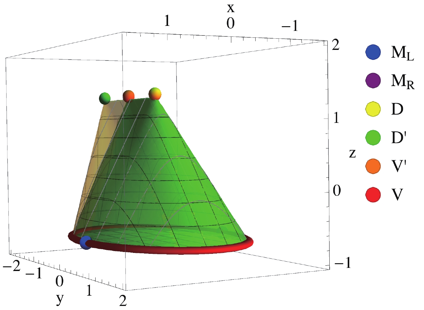
Figure 2. (color online) Three-dimensional cross section of the convex cones
${\cal C}$ (yellow, bigger cone) and${\cal C}_1$ (green). The cross section is taken to be perpendicular to the direction$(1,1,0,1)$ . The three axes x, y, and z are defined along the$(1,-1,0,0)$ ,$(0,0,1,0)$ , and$(-1,-1,0,2)$ directions, respectively.An important observation is that, for tree level UV-completions, all
$ \vec c^{\ (8)}_X $ listed in Eq. (31) are extremal, i.e., they cannot be split as positive sums of other elements in$ {\cal{C}}_1 $ . Beyond this tree-level assumption (i.e., on the yellow$ {\cal{C}} $ cone), only one of the points,$ V' $ , becomes non-extremal. This is related to the appearance of one extra irrep,$ D' $ , so that$ V' $ can now be expressed as a positively weighted sum of$ D' $ and D. The new irrep$ D' $ can be interpreted as a new vector$ V_{D'} $ that couples as a dipole moment so that it cannot be generated by a tree-level UV completion (and is thus external to the$ {\cal{C}}_1 $ cone).Let us now assume that the Wilson coefficients can all be determined experimentally, with the measurement being denoted
$ \vec C_{\exp} $ . We can thus write$ \vec C_{\exp} = \sum\limits_X w_X \vec c^{\ (8)}_X . $

(34) What can we learn about the particles living in the UV of the theory, and how important are their effects? In other words, how could we obtain information on the
$ w_X $ parameters from the knowledge of the l.h.s. of the above equation? One may naively believe that this is not possible as there is an infinite number of ways to arrange UV particles to satisfy the above equation. Surprisingly, the positivity nature of the dimension-8 coefficient parameter space allows for interesting inferences. While in principle,$ \vec C_{\exp} $ can only be measured up to some uncertainties, we neglect the latter in this section. We refer instead to Section V.C for a more realistic example including those uncertainties, in which we demonstrate that this does not prevent us from using positivity to infer knowledge on the existence of potential BSM particles and their properties.We start by considering a measurement of
$ \vec C_{\exp} $ that would be found parallel to a$ \vec c^{\ (8)}_{X'} $ vector extremal in$ {\cal{C}}_1 $ . In this case,$ \vec C_{\exp} = \lambda \vec c^{\ (8)}_{X'} $ so that the only solution to Eq. (34) is$ {w_X} = \left\{ {\begin{array}{*{20}{l}} {\lambda \quad }&{{\rm{if}}\;X = X'\;,}\\ 0&{{\rm{otherwise}}\;.} \end{array}} \right. $

(35) This follows from the definition of an extremal ray that cannot be written as a positively weighted sum of other cone elements. In other words, if the dimension-8 operators have been generated by particles living in a single representation, a “precise” measurement of the dimension-8 Wilson coefficients could not only confirm this hypothesis but also exclude the potential existence of any other particles without making any assumption on the BSM details, and thus falsifying other alternative hypotheses. This feature can be traced back to the fact that all
$ \vec c_X^{\ (8)} $ live in a salient cone.In contrast, the above inference is not possible when one truncates the SMEFT expansion at the dimension-6 level, as there would always be an infinite number of positive solutions (with
$ w_X\geqslant 0 $ ) for Eq. (34). For example, one could consider a D scalar and a$ V' $ vector with arbitrarily large contributions that cancel each other out completely, or similarly an$ M_L $ scalar and a V vector with$ \kappa = 0 $ . This originates from the fact that the allowed values for the dimension-6 Wilson coefficients do not live within a salient cone, and hence, there are always several ways to organize them to reproduce any measured coefficient value. Therefore, an interpretation at the dimension-6 level can only be achieved under specific model assumptions and thus fits within a top-down study.More generally, if
$ \vec C_{\exp} $ is not extremal, one can still set upper limits on the weights$ w_X $ by starting from$\vec C(\lambda)\equiv \vec C_{\exp}-\lambda \vec c_{X'} = \sum\limits_{X\neq X'} w_X\vec c_X+(w_{X'}-\lambda)\vec c_{X'} . $

(36) Since
$ \vec C(0)\in {\cal{C}}_1 $ and$ \lim_{\lambda\to+\infty}\vec C(\lambda) \notin {\cal{C}}_1 $ (by the definition of a salient cone), there exists a maximum value$ \lambda_{\max} $ below which we have$ \vec C(\lambda)\in {\cal{C}}_1 $ . This provides an upper bound for$ w_{X'} $ , as if$ w_{X'}>\lambda_{\max} $ , then we can find a$ \lambda $ value such that$ w_{X'}>\lambda>\lambda_{\max} $ and for which$ \vec C(\lambda)\notin {\cal{C}}_1 $ (as$ \lambda> \lambda_{\max} $ ), yielding a contradiction. Physically, this indicates that, if we remove some$ X' $ contribution from$ \vec C_{\exp} $ , the remaining vector still consists of a positively weighted sum that should satisfy tree-level positivity by belonging to$ {\cal{C}}_1 $ . Therefore, the largest$ X' $ contribution that could be removed from$ \vec C_{\exp} $ without spoiling these bounds provides an upper bound on$ w_{X'} $ . This can then be iteratively used to set upper limits on the existence of all types of particles. Again, such an inference is not possible at the dimension-6 level, as there is no equivalent to$ {\cal{C}}_1 $ .Setting an upper limit on
$ w_X $ is important, as this limit applies to not only the total contribution from all particles of a given type but also each individual generation of a particle of this type. While this is evident for$ X\neq V $ , as$ 0\leqslant \frac{g_{Xi}^2}{M_{Xi}^4}\leqslant \sum\limits_i\frac{g_{Xi}^2}{M_{Xi}^4} = w_{X} , $

(37) this is also true for
$ X = V $ , as all$ \vec c_{V(\kappa)}^{\ (8)} $ live on a circular cone.A similar reasoning can be achieved beyond the tree level by replacing the
$ {\cal{C}}_1 $ cone by$ {\cal{C}} $ . Hence, upper limits can be set on the existence of states in all possible irreps$ \bf r $ and on an individual generation of particles lying in this irrep. Moreover, this includes both one-particle and multi-particle states (which yield loop-level generated coefficients), as their contributions are always individually positive.In summary, we have shown so far that, in contrast to the dimension-6 case, a measurement of the dimension-8 Wilson coefficients would allow us to rule out or at least place a lower bound on the mass scale of each individual particle of a given type X without any model assumption. If a deviation from the SM is observed, these universal bounds narrow down the possible range of UV-complete BSM models that should be considered. On the contrary, if no deviation is observed, then model-independent exclusion limits on the BSM states can be set, at least up to certain scales depending on the precision of the measurement. This last point is crucial as a test of the SM. If no significant deviation from the SM is observed at future colliders, a global fit of the dimension-6 Wilson coefficients would only allow to set limits on the dimension-6 contributions without being able to further exclude the possibility that BSM exists in a way yielding the suppression of any dimension-6 effect (by virtue of cancellations or symmetry reasons). Hence, such a fit would not be sufficient to confirm the SM. In contrast, a global fit of the coefficients of operators ranging up to dimension-8 would allow for not only the extraction of limits on the coefficients, but, more importantly, also the exclusion of the existence of BSM states, thus confirming the SM.
The illustration presented in this section is based on the assumption of weakly-coupled UV completions. However, the conclusions hold in general, as positivity implies that any UV completion of the SM must lead to some non-vanishing dimension-8 effects. This should further motivate the study of dimension-8 operators through precision physics in the future.
On different grounds, we indicate that it is also possible to set some lower limits on a particular weight
$ w_{X'} $ . To this end, we introduce the convex cone$ {\cal H}_{X'} $ defined by all$ \vec c_X $ vectors different from$ \vec c_{X'} $ , using instead the opposite of the latter as a last element to define the cone,$ {\cal H}_{X'} = {\rm{cone}}\left( \left\{ \vec c_{X\neq X'}, -\vec c_{X'}\right\}\right). $

(38) In the case where
$ \vec C_{\exp}\notin {\cal H}_{X'} $ , the lower limit on$ w_{X'} $ is given by the minimum$ \lambda $ value such that$ \vec C_{\exp}- $ $\lambda\vec c_{X'}\in {\cal H}_{X'} $ . However, this also applies at the dimension-6 level. -
In this section, we pioneer a realistic study of the feasibility of positivity tests at future colliders and investigate the possibility of inferring or excluding the existence of new physics in the UV. However, a more accurate determination of the impact of dimension-8 contributions at future colliders (and the estimation of their reach in the corresponding Wilson coefficient parameter space) is beyond the scope of this paper. Hence, we have performed several simplifications in our analysis. We first restrict ourselves to parton-level simulations and omit any higher-order corrections and initial-state radiation effect. Second, we assume an ideal detector and thus ignore any reconstruction and experimental effect.
We utilize FeynRules [34] to generate a UFO model [35] including all the operators introduced in Section II so that we could simulate
$ e^+e^-\to e^+e^- $ scattering with MadGraph5_aMC@NLO [36]. We analyze the resulting parton-level events with MadAnalysis 5 [67-69], which is also used to define an appropriate fiducial volume. The latter embeds a selection on the final-state lepton transverse momentum of$ p_T>5 $ GeV and on their pseudorapidity of$ |\eta|<5 $ . We then split the phase space into 25 bins in$ \cos\theta $ , with$ \theta $ being the lepton scattering angle. Moreover, we discard the most forward bin, as it corresponds to the bin where the SM contribution blows up.Given that
$ e^+e^-\to e^+e^- $ cross section measurements at LEP2 reached a precision of approximately 2%, we assume that the systematic uncertainties could be controlled at the 1% level for each$ \cos\theta $ bin. In addition, we include statistical uncertainties that we estimate as$ \sqrt{N} $ , where N is the projected number of events in a given bin. We have finally verified the consistency of the simulation results with analytical calculations.We have considered several future lepton collider pro-jects, mostly following the setups presented in Ref. [70]. However, we have omitted any operation run at the Z-pole, as the cross section is dominated by the Z-resonance contribution instead of any potential four-fermion operator effect. In addition, for the ILC case, we focus on a possible upgrade at a center-of-mass energy of 1 TeV [31]. We refer to Table 2 for details on the center-of-mass energies, luminosities, and beam polarization options of all collider configurations studied in this paper.
Scenario Beam polarization $P(e^-,e^+)$ 

Runs (luminosity @ energy), [ab−1] @ [GeV] 1 2 3 4 CEPC None 2.6@161 5.6@240 FCC-ee None 10@161 5@240 0.2@350 1.5@365 ILC-500 (−80%, 30%) 0.9@250 0.135@350 1.6@500 (80%, −30%) 0.9@250 0.045@350 1.6@500 ILC-1000 (−80%, 30%) 0.9@250 0.135@350 1.6@500 1.25@1000 (80%, −30%) 0.9@250 0.045@350 1.6@500 1.25@1000 CLIC (−80%, 0%) 0.5@380 2@1500 4@3000 (80%, 0%) 0.5@380 0.5@1500 1@3000 Table 2. Different future collider operation runs considered in this study, presented together with the associated center-of-mass energy, expected luminosity, and beam polarization setup (if relevant).
-
The
$ e^+e^-\to e^+e^- $ differential cross section can be parameterized as a polynomial in the higher-dimensional operator coefficients, as shown in Eq. (5). In the following, we denote by$ \vec C $ the entire set of coefficients,$ \vec C = (C_{ee},C_{el},C_{ll},C_1,C_2,C_3,C_4)\ , $

(39) and the effective cutoff scale
$ \Lambda $ is set to 1 TeV, unless specified otherwise. To evaluate the constraining power and sensitivity of the future collider under consideration to the higher-dimensional operators introduced in Section II, we built a$ \chi^2 $ function,$ \chi^2\left(\vec C,\vec C_0\right)\ , $

(40) in which we assume that a would-be observation
$ \vec C $ agrees with the theoretical predictions associated with some reference hypothesis$ \vec C = \vec C_0 $ . The allowed range for$ \vec C $ at some confidence level can then be determined by the$ \vec C $ values for which$ \chi^2\leqslant \chi^2_c $ , where$ \chi^2_c $ represents the critical$ \chi^2 $ value allowing to reach an agreement with$ \vec C_0 $ at the required confidence level. For the remainder of this paper, all the presented limits have been evaluated at$ 2\sigma $ .In the case where the would-be observations would agree with the SM, limits on the four-electron Wilson coefficients can be set by enforcing
$ \chi^2(\vec C,0) \leqslant \chi^2_c $ . These limits, cast under a$ C\in [C_{\rm min},C_{\rm{max}}] $ form for each coefficient, reflect the sensitivity of the future lepton colliders to the considered operators. They can be further converted into the new physics characterization scale$ \Lambda_c $ that represents the BSM scale that is reachable at the various colliders. We define$ \Lambda_c $ by$\begin{aligned}[b] {{\rm{dimension - 6:}}\quad }&{{\Lambda _c} \equiv \dfrac{\Lambda }{{\sqrt {\dfrac{{{C_{{\rm{max}}}} - {C_{{\rm{min}}}}}}{2}} }}\;,}\\ {{\rm{dimension - 8:}}\quad }&{{\Lambda _c} \equiv \dfrac{\Lambda }{{\sqrt[4]{{\dfrac{{{C_{{\rm{max}}}} - {C_{{\rm{min}}}}}}{2}}}}}\;,} \end{aligned}$

(41) in the dimension-6 and dimension-8 cases, respectively.
These scales are depicted in Fig. 3. For each collider and each specific coefficient (i.e., in each column), the lighter color represents the individual limit obtained when all other coefficients are enforced to vanish, whereas the darker color represents the marginalized limit obtained where all other coefficients are left floating. For an easy comparison of the strengths of the various machines, we show through the darkest color the largest collider center-of-mass energy reachable for each collider.
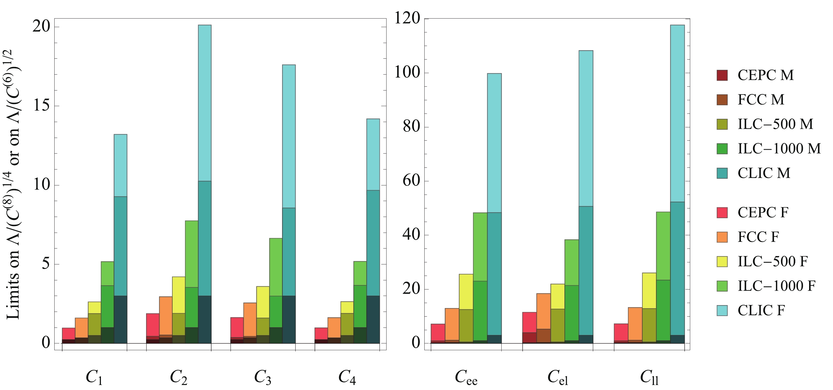
Figure 3. (color online) Limits on the new physics characterization scale
$\Lambda_c$ (in TeV) for the various considered future lepton colliders. "M" denotes marginalized limits (all other coefficients being floating), whereas "F" denotes individual limits (all other coefficients being vanishing). In addition, we represent by the darkest color the largest center-of-mass energy of each collider project.In the case of the dimension-6 operator coefficients, we observe that all future lepton colliders are sensitive to very large new physics scales (given in terms of
$ \Lambda_c $ ). Those scales are indeed typically approximately 1 or 2 orders of magnitude larger than the collider center-of-mass energy. This is more or less expected, given that LEP2 already reached a sensitivity of a few TeV on those operators [71].For the dimension-8 operators, the individual sensitivities range from
$ {\cal O}(1) $ (CEPC) to$ {\cal O}(10) $ (CLIC) TeV. They are roughly a factor of 5 larger than the collider center-of-mass energy, which also indicates that the EFT approach is robust in the considered context. However, the more reliable limits are those obtained through marginalized bounds. They are reduced by a factor of a few when compared with the individual limits. Nevertheless, for all scenarios, the corresponding$ \Lambda_c $ is sufficiently higher than the collider energy, except for the$ O_1 $ and$ O_4 $ operators in the CEPC and FCC-ee cases. Here, the$ \Lambda_c $ scale is observed to be slightly lower than the highest expected center-of-mass energy (see the discussion below). In general, the EFT validity is thus not an issue for$ {\cal O}(1) $ BSM couplings, and the dimension-8 effects can be identified even in the presence of dimension-6 operators.For all considered circular colliders, the marginalized limits for the operators
$ O_1 $ ,$ O_4 $ ,$ O_{ee} $ , and$ O_{ll} $ are much weaker than their corresponding individual limits. This originates from an accidental degeneracy between the linear-level contributions of the$ LLLL $ and$ RRRR $ types of operators. For a slightly larger electroweak mixing angle such that$ \sin^2\theta_W = 0.25 $ , the$ Zee $ coupling in the SM would be of a purely axial-vector nature, yielding identical$ e^+_Le^-_L\to e^+_Le^-_L $ and$ e^+_Re^-_R\to e^+_Re^-_R $ cross sections (including the photon and Z-boson exchanges, as well as their interference). In this hypothetical case, the$ O_{ee} $ /$ O_{ll} $ and$ O_1 $ /$ O_4 $ contributions cannot be distinguished, unless beam polarization is used (so that the linear collider sensitivity is much stronger). In practice,$ \sin^2\theta_W = 0.234 $ (from$ m_Z = 91.1876 $ GeV and$ \alpha = 1/127.9 $ ), and hence, this degeneracy is not exact. However, this leads to an almost flat direction in the Wilson coefficient parameter space, or equivalently to large differences between the individual and marginalized limits for the$ O_1 $ ,$ O_4 $ ,$ O_{ee} $ , and$ O_{ll} $ operators.As our fit is at the quadratic level for the dimension-6 operator coefficients,
$ O_{ee} $ and$ O_{ll} $ are thus essentially constrained by their quadratic contributions. On the other hand,$ O_1 $ and$ O_4 $ are only included at the linear level so that some caution is required when interpreting the corresponding limits. It is observed that the numerical simulations are not reliable in this case, as statistical fluctuations may artificially lift the degeneracy. Therefore, we have employed our analytical computations for those two operators and the two circular collider cases. We have additionally verified that, using$ m_Z $ ,$ G_F $ , and$ m_W $ as electroweak input parameters (yielding$ \sin^2\theta_W = 0.223 $ ), the marginalized limits on$ O_1 $ and$ O_4 $ are only impacted at the level of approximately 10%, all other limits being stable.Finally, to estimate the error due to the SMEFT truncation at
$ {\cal O}(\Lambda^{-4}) $ in Eq. (5), we have assessed the impact of the next order contributions, namely the interferences between the dimension-6 and dimension-8 operators and the quadratic contributions in the dimension-8 operators. The resulting changes in Fig. 3 are quite mild. The limits at the circular colliders are modified by less than 10%, whereas those associated with the linear colliders are negligibly affected. Therefore, our truncation at$ {\cal O}(\Lambda^{-4}) $ is reliable, and any higher-order contributions will be ignored in the remainder of this paper. -
We now assume that some would-be observation at future colliders in
$ e^+e^-\to e^+e^- $ scattering data is consistent with a coefficient value hypothesis$ \vec C_0 $ . We aim at investigating what we could learn, from this measurement, about the potential amount of positivity violation$ \Delta^{-1} $ .We start from the fact that, for any given
$ \vec C_0 $ , a measurement indicates that the true coefficient vector$ \vec C $ of the theory is constrained by$ \chi^2({ \vec C,\vec C_0})<\chi^2_c $ at some confidence level. We can thus deduce a confidence interval for the amount of positivity violation,$ \Delta^{-1}\in \big[\Delta^{-1}_{\rm{low}},\Delta^{-1}_{\rm{high}}\big]\ , $

(42) with
$ \begin{aligned}[b] \Delta^{-1}_{\rm{low}} = &\ \min\limits_{\chi^2({ \vec C,\vec C_0})\leqslant\chi^2_c} \left(\frac{\delta(\vec C)^\frac{1}{4}}{\Lambda}\right),\\ \Delta^{-1}_{\rm{high}} = &\ \max\limits_{\chi^2({ \vec C,\vec C_0})\leqslant\chi^2_c} \left(\frac{\delta(\vec C)^\frac{1}{4}}{\Lambda}\right). \end{aligned} $

(43) We focus on
$ \Delta^{-1}_{\rm{low}} $ , which is a conservative estimate of$ \Delta^{-1} $ , so that we could conclude about the existence of some positivity violation if$ \Delta_{\rm{low}}^{-1}>0 $ .We consider four benchmarks that differ by the
$ \vec C_0^{(8)} = (C_1,C_2,C_3,C_4) $ choice,$ \begin{aligned}[b] B_1:\ & \vec{C}_0^{(8)} = (0,0,3,1.2),\\ B_2:\ & \vec{C}_0^{(8)} = (0,0.3,0.2,0),\\ B_3:\ & \vec{C}_0^{(8)} = (0,0.015,0.015,0),\\ B_4:\ & \vec{C}_0^{(8)} = (0,0,0.0006,0.00015). \end{aligned} $

(44) The corresponding amount of positivity violation
$ \Delta^{-1} $ is given in Table 3, together with the$ \Delta^{-1}_{\rm{low}} $ values that could be reached at each considered collider scenario when assuming that the measurements are consistent with the$ B_i $ hypothesis. Those results have been estimated by marginalizing over all dimension-6 four-electron operators, so that they can be taken as conservative.$\Delta^{-1}$ 

$\Delta^{-1}_{\rm{low}}$ 

CEPC FCC-ee ILC-500 ILC-1000 CLIC $B_1$ 

1.48 0 0.86 1.45 1.47 1.48 $B_2$ 

0.74 0 0 0.66 0.73 0.74 $B_3$ 

0.35 0 0 0 0.29 0.35 $B_4$ 

0.16 0 0 0 0 0.10 Table 3. Amount of positivity violation
$\Delta^{-1}$ associated with each considered benchmark and the corresponding$\Delta^{-1}_{\rm{low}}$ bound that could be obtained at each collider scenario. The results are all given in TeV-1 and at the 95% confidence level.The four points have been chosen to illustrate an increasing sensitivity to positivity violations at the five collider scenarios under consideration. The
$ B_1 $ setup corresponds to a violation arising at a scale of approximately 700 GeV, which can be observed at the$ 2\sigma $ level by all studied lepton colliders except for the CEPC. The$ B_2 $ point allows for the observation of a positivity violation at scales of approximately 1.4 TeV, which can only be observed at future linear colliders. Finally, the$ B_3 $ and$ B_4 $ benchmarks induce positivity violation scales that go up to 2.9 and 6.4 TeV, respectively, to which only the ILC with an energy upgrade at 1 TeV and CLIC are expected to be sensitive.To obtain a more intuitive picture, we present a slice of the dimension-8 Wilson coefficient parameter space for the two benchmarks
$ B_3 $ and$ B_4 $ in Fig. 4. In the two subfigures, we depict by a light green area the parameter space region allowed by the positivity bounds. Moreover, we indicate through light gray contours the amount of positivity violation arising in the remainder of the parameter space, using the dimensionless parameter$ \delta(\vec C^{(8)}) = ({1\ {\rm{TeV}}}/{\Delta})^4 $ . Consistent with the definition of these two benchmarks in Eq. (44), the other two dimension-8 coefficients ($ C_1 $ and$ C_4 $ for the$ B_3 $ scenario and$ C_1 $ and$ C_2 $ for the$ B_4 $ scenario) are taken as vanishing. The limits that could be imposed from measurements at various lepton colliders are given by solid and dashed contours. They respectively correspond to a derivation including a marginalization over the dimension-6 Wilson coefficients (labeled by “M”) or after fixing them to zero (labeled by “F”).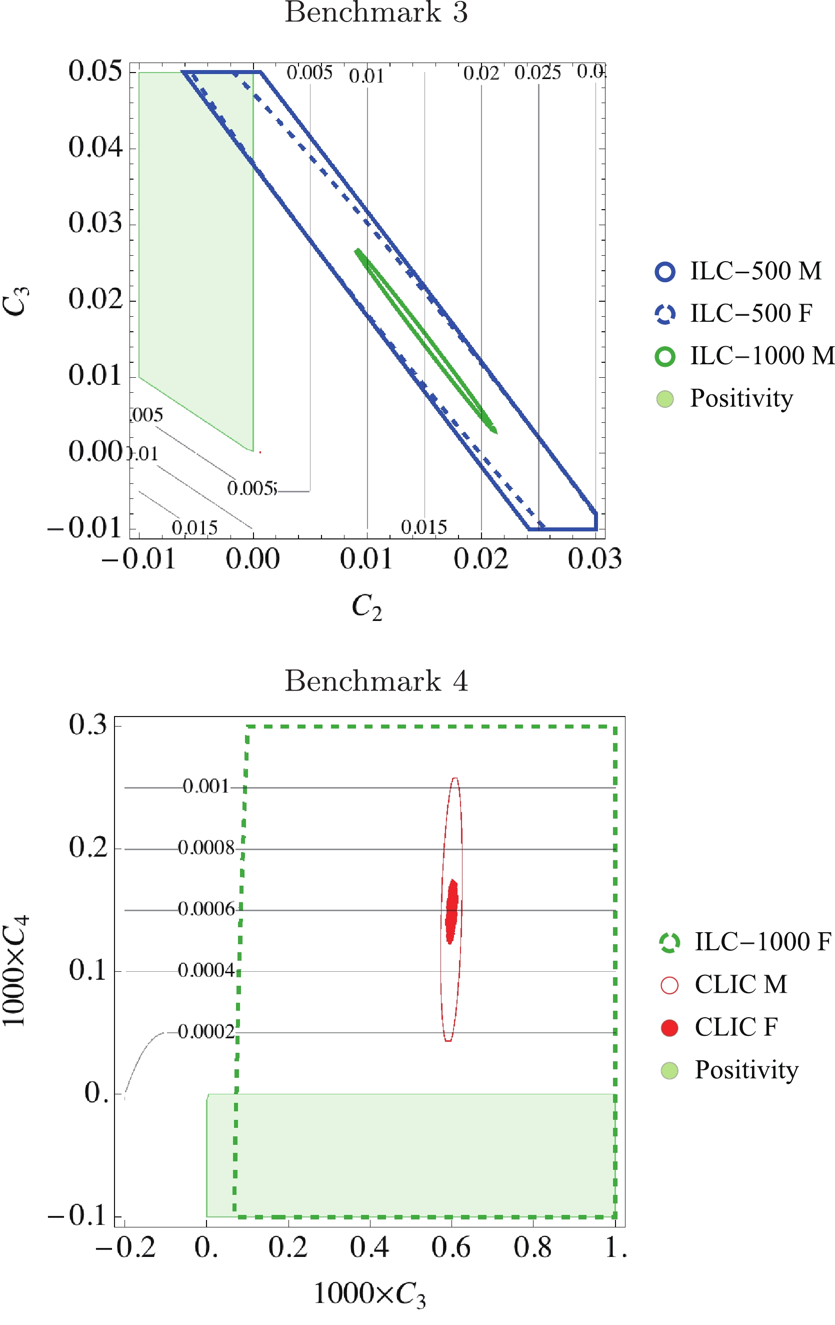
Figure 4. (color online) Bounds on the pairs of dimension-8 operator coefficients that are relevant for the benchmark points
$B_3$ (upper) and$B_4$ (lower). In each case, the other two dimension-8 coefficients are set to 0, as in the benchmark scenario definitions from Eq. (44), whereas the dimension-6 coefficients are either marginalized over (M, solid) or fixed to 0 (F, dashed). We show the$2\sigma$ expectations for the reach of different future lepton collider projects as colored contours, and the light green area represents the parameter space region allowed by the positivity bounds. Outside this area, the gray isolines depict the dependence of the$\delta(\vec C)= ({1\ {\rm{TeV}}}/{\Delta})^4$ quantity, which is thus used as an estimate for the amount of positivity violation, on the coefficients.We observed differences between the solid and dashed contours, which indicates that there are correlations between the impacts of the dimension-6 and dimension-8 operators. Nevertheless, even after marginalizing the dimension-6 coefficients, a sensitivity to the dimension-8 operators remains, as illustrated in the case of the ILC-1000 collider (for the
$ B_3 $ benchmark) and CLIC (for the$ B_4 $ benchmark). The entire$ 2\sigma $ contours indeed lie outside the positivity area so that a positivity violation could be confirmed, regardless of the existence of any dimension-6 effect. On different grounds, notably, the fact that the marginalized limits do not overlap with the positivity area does not guarantee a potential confirmation of$ \Delta^{-1}_{\rm{low}}>0 $ , as we only focus here on a slice of the full dimension-8 coefficient space.It is evident that a large
$ \Delta^{-1} $ value has a better chance to be confirmed experimentally, but this also depends on the actual values of all the dimension-8 coefficients. Any given amount of violation may indeed indicate different regions of the parameter space, with some of them being phenomenologically easier to detect than others. An interesting question would be as follows: how large should the amount of violation$ \Delta^{-1} $ be for a collider to have a significant chance to confirm it?A quantitative and accurate answer is difficult to provide, due to the quartic nature of our
$ \chi^2 $ fit and the discontinuous nature of the$ \delta(\vec C) $ function. We present below a tentative answer by sampling the dimension-6 and dimension-8 parameter space with a Monte Carlo method and assessing, for each sampled configuration, the$ (\Delta^{-1}, \Delta^{-1}_{\rm{low}}) $ values. After restricting the values of the dimension-6 coefficients to the order of 0.1 TeV$ ^{-1} $ so that they are roughly consistent with LEP-2 constraints [71], we show our results in Fig. 5. This figure shows the correlation between the violation scale$ \Delta^{-1} $ and its$ 2\sigma $ lower bound$ \Delta^{-1}_{\rm{low}} $ as obtained by would-be measurements at the CEPC, FCC-ee, ILC-500, ILC-1000, and CLIC colliders. In other words, the results indicate the experimental sensitivity to some positivity violation scale$ \Delta $ at a given collider.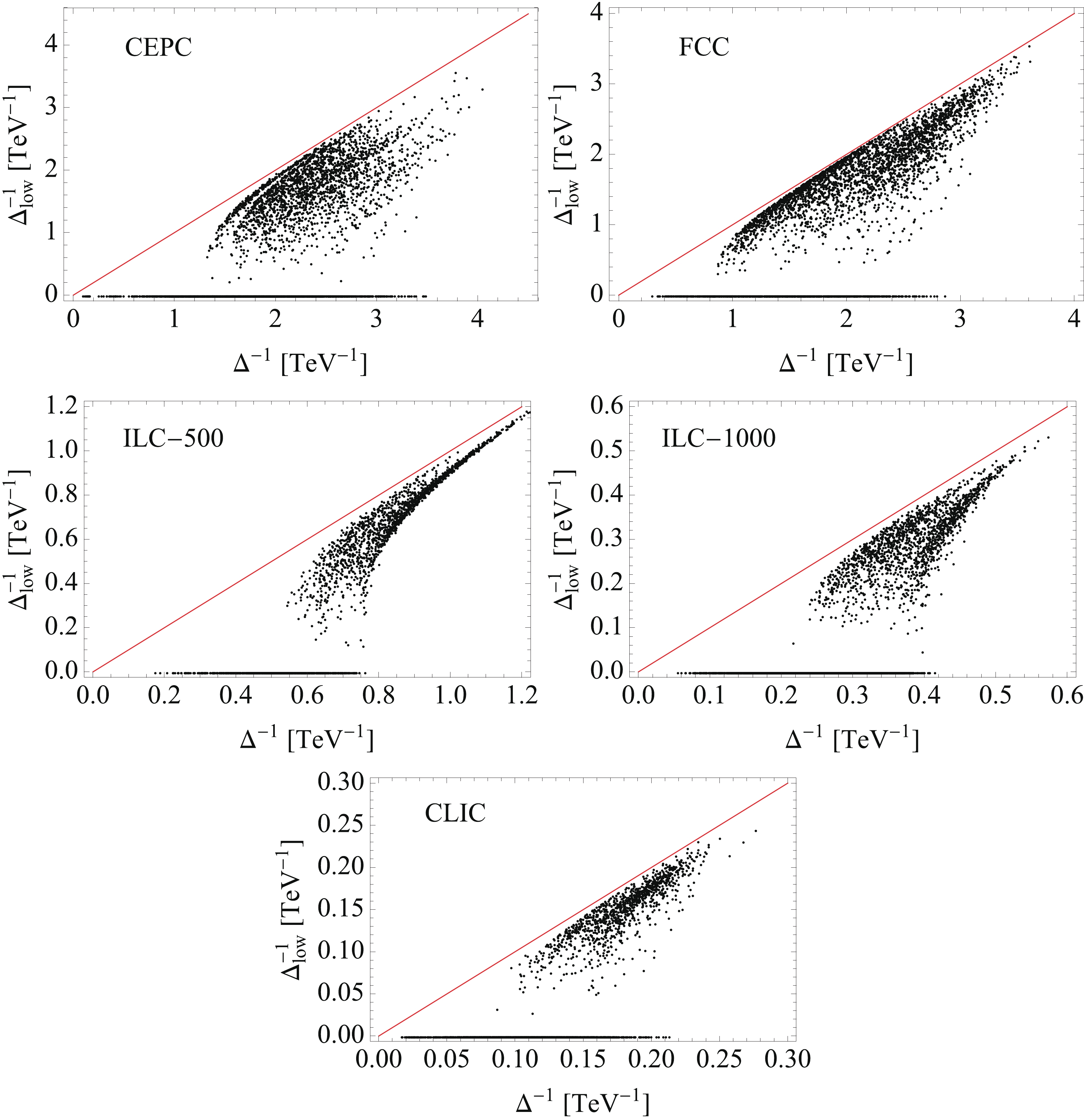
Figure 5. (color online) Correlations between the amount of positivity violation (
$\Delta^{-1}$ ) and the maximal sensititivity that can be reached at a given future lepton collider ($\Delta^{-1}_{\rm{low}}$ ). We present results for the CEPC (upper left), FCC-ee (upper right), ILC (center), and CLIC (lower) colliders, and each represented point has been obtained through a Monte Carlo sampling of the dimension-6 and dimension-8 Wilson coefficient parameter space.Two particularly important features can be extracted. First, the smallest
$ \Delta^{-1} $ value that corresponds to a nonzero$ \Delta_{\rm{low}}^{-1} $ value defines the minimum amount of positivity violation that is, in principle, observable at each collider. This corresponds to scales of 0.7, 1.2, 1.8, 4.2, and 11 TeV for the CEPC, FCC-ee, ILC-500, ILC-1000, and CLIC colliders, respectively. These scales are much higher than the corresponding (highest) expected center-of-mass energy, and thus, the positivity tests are observed to be phenomenologically feasible for all five machines. Moreover, a positivity violation that should occur at or below these scales thus has a chance to be detected. Second, the largest$ \Delta^{-1} $ value associated with a zero$ \Delta_{\rm low}^{-1} $ value corresponds to the minimum guaranteed observable amount of positivity violation, regardless of the actual coefficient values. This corresponds to scales of 0.3, 0.36, 1.3, 2.4, and 4.8 TeV for the above five colliders, respectively. These scales are slightly higher than, but comparable to, the corresponding collider energies. Equivalently, a violation occurring at these scales yields a guaranteed$ 2\sigma $ observation.Those possible evaluations of
$ \Delta $ for$ e^+e^-\to e^+e^- $ scattering at various colliders serve as a proof of concept for how well collider physics can be used as a novel means to probe the fundamental principles of QFT in a model-independent way. As we have argued in Section III.B, the scale$ \Delta $ could be viewed as a rough estimate for the scale$ \Lambda_* $ (with$ \Lambda_*\gtrsim \Delta $ ) connected to the violation of the fundamental QFT principles. The results obtained in the present section demonstrate that scenarios for which$ \Delta $ lies in a range of$ {\cal O}(1)-{\cal O}(10) $ TeV have a chance to be confirmed.Therefore, we conclude that future
$ e^+e^- $ colliders will be able to test the fundamental principles of QFT up to a scale of the order of 10 TeV or even beyond, depending on the exact nature of BSM physics. Moreover, if positivity violation is observed, then unconventional model building approaches, such as those discussed in Section III.B, will be necessary. The measurement of the corresponding$ \Delta $ value will, in this case, provide an important guidance. However, the actual connection between$ \Delta $ and the scale$ \Lambda_* $ at which the QFT core principles are violated should be studied on a model-by-model basis. -
In Section IV, we have argued that the positive nature of the dimension-8 parameter space can be used to infer or exclude the possible existence of new physics states in the UV, independent of the nature of the new physics model. In this section, this argument is demonstrated with realistic examples.
We first consider an extension of the SM where the new physics sector of the theory solely includes a D-type scalar (see Table 1). For an illustrative benchmark scenario, we fix its mass to 2 TeV, its coupling
$ g_D $ defined in Eq. (28) to 0.8, and focus on the ILC-1000 collider. Integrating this heavy field out generates two higher-dimensional operators: one of dimension-6 and one of dimension-8. The associated Wilson coefficients can be parameterized in terms of the$ \vec C_0^{(6)} $ and$ \vec C_0^{(8)} $ vectors of Eq. (4),$\begin{aligned}[b] & \vec C_0^{(6)} = (0,-0.08, 0)\ , \\ &\vec C_0^{(8)} = (0,0,0.04,0)\ . \end{aligned}$

(45) The
$ \chi^2 $ -fit introduced in the previous section allows for the identification of the coefficient space region that would be reachable from$ e^+e^-\to e^+e^- $ measurements at the ILC-1000, assuming a$ \vec C_0 $ theory hypothesis. Such a region is defined by the$ \vec C $ values yielding$ \chi^2(\vec C,\vec C_0)\leqslant \chi_c $ so that one can extract marginalized limits, at the 95% confidence level, on all coefficients,$ \begin{array}{*{20}{l}} {C_{ee}} = 0 \pm 0.0024,\qquad \;{C_{el}} = - 0.08 \pm 0.0035,\\ {C_{ll}} = 0 \pm 0.0023,\\ {C_1} = 0 \pm 0.0074,\qquad \;\;{C_2} = 0 \pm 0.0077,\\ {C_3} = 0.04 \pm 0.020,\qquad {C_4} = 0 \pm 0.0071. \end{array}$

(46) As already mentioned above, the interpretation of these results cannot be model-independent at the dimension-6 level. For example, assuming that the SM is only supplemented by a D-type scalar generating the
$ O_{el} $ operator, one would then obtain as a bound on the new physics mass scale$ M_D/g_D\in [2.45,2.56]\ {\rm{TeV}} . $

(47) On the other hand, if we assume that the SM is extended by both a D scalar and a
$ V' $ vector (coupling with a strength$ g_{V'} $ as in Eq. (28)), then we can only conclude that$\frac{g_D^2}{2M_D^2}-\frac{g_{V'}^2}{M_{V'}^2} = 0.08\pm0.0035\ {\rm{TeV}}^{-2}. $

(48) Moreover, it is impossible to disentangle the individual contributions from each particle type, and the situation only worsens by making the model more complex due to other ways by which similar cancellations may occur.
This shows that conclusions can only be drawn under very specific BSM assumptions, as we do not know a priori the exact particle content of the theory. Thus, this kind of interpretation is only practical for top-down studies of specific UV models, as for example the one carried out in Ref. [14].
One might naively believe that this lack of information is due to the fact that, at the dimension-6 level, we only measure three coefficients, whereas the number of possible UV states is infinite (as there can be several V particles with different
$ \kappa_i $ couplings). Consequently, including dimension-8 operators as well would not help significantly. On the contrary, this is not the case. As we have argued in Section IV, the positive nature of the dimension-8 space allows us to set an upper limit on the total contribution (or weights$ w_X $ ) of any given type of particles X.For example, for a particle species
$ X' $ , we can determine the$ \lambda_{\max} $ value defined by$ \lambda_{\max} \equiv \max\limits_\lambda \Big[ \vec C_{\exp}^{(8)}- \lambda \vec c_{X'}^{\ (8)}\in {\cal{C}}\Big] , $

(49) where
$ \vec C_{\exp}^{(8)} $ denotes the projected measurements of the Wilson coefficients at some collider, the vector$ \vec c^{\ (8)}_{X'} $ is given, for any specific particle type, by Eq. (31), and$ {\cal{C}} $ consists of the cone generated from the entire ensemble of$ \vec c^{\ (8)}_X $ vectors. Therefore, the$ \lambda_{\max}\vec c^{\ (8)}_{X'} $ quantity indicates an upper bound on the contribution to the dimension-8 coefficients that can arise from any set of$ X' $ states.This has a simple interpretation at the tree level. If we remove from
$ \vec C_{\exp} $ the contribution of all BSM$ X' $ states, then the remaining quantity is still a positively weighted sum of the contributions of particles from all types different from$ X' $ . Consequently, this should fall within$ {\cal{C}} $ . Therefore, the largest amount that can be removed from$ \vec C_{\exp} $ in the$ \vec c^{\ (8)}_{X'} $ direction without leaving the cone$ {\cal{C}} $ provides the upper bound on the total contribution of$ X' $ states to$ \vec C_0 $ . Moreover, this still holds beyond the tree level, as both the existence of the cone$ {\cal{C}} $ and the reasoning provided in Section IV are valid for all orders.However, the above statement assumes that
$ \vec C_{\exp}^{(8)} $ is ideally determined, without any uncertainty. In practice, this is not the case, so that one could question the impact of the experimental uncertainties. In our example, the measurement suggests that$ \vec C^{(8)} $ falls in the dimension-8 coefficient parameter space region defined by$ \chi^2(\vec C,\vec C_0)\leqslant \chi_c^2 $ . Therefore, the experimental uncertainties can be naturally accounted for by evaluating the maximum of all$ \lambda_{\max} $ derived for all allowed$ \vec C^{(8)} $ values in this region,$ \lambda_{\max} \equiv \max\limits_\lambda \Big[ \vec C^{(8)}- \lambda \vec c_{X'}^{\ (8)}\in {\cal{C}};\ \chi^2\big(\vec C, \vec C_0\big)\leqslant \chi^2_c \Big] \ , $

(50) where
$ \vec C\equiv \{\vec C^{(6)}, \vec C^{(8)}\} $ and$ \vec C_0\equiv \{\vec C_0^{(6)}, \vec C_0^{(8)}\} $ . Thus, we have also incorporated the dimension-6 coefficients that are marginalized over.Let us now apply this general procedure to the benchmark scenario defined in Eq. (45). As the coefficients
$ \vec C^{(6)}_0 $ and$ \vec C^{(8)}_0 $ are known, the$ \chi^2 $ function can be built from the projected measurement. Eq. (50) therefore expresses a constrained optimization problem. For example, for a$ M_V $ new physics vector state with$ \kappa = 1 $ (as defined in Table 1 and Eq. (28) so that its couplings to the electron are of a vector-like nature), we find$ \lambda_{\max} = 0.0054 $ . Thus, the$ M_V $ contribution to$ \vec C^{(8)} $ is constrained to be less than approximately 10% in magnitude. In terms of the new physics mass and coupling, this is given by$ \frac{M_{V}}{\sqrt{g_{V}}}\geqslant 3.7\ {\rm{TeV}} .$

(51) We emphasize that such a bound is different from the dimension-6 case expressed in Eqs. (47) and (48). The constraint of Eq. (51) is indeed universal and excludes any possible V-type particle featuring a coupling to electrons of strength
$ \kappa = 1 $ with properties violating the bound, without relying on any specific model assumptions.For an intuitive understanding of this universal bound, we investigate what happens when
$ \lambda $ varies toward$ \lambda = \lambda_{\max} $ geometrically. To this end, we identify two points in the dimension-8 coefficient space:$ \vec C_{\rm{max}}^{(8)} $ and$ \vec C_{\rm{max}}^{(8)}-\lambda_{\rm{max}}\vec c_{V}^{\ (8)} $ . The former corresponds to a saturation of the experimental bounds, whereas the latter corresponds to a saturation of the positivity bounds. This is represented in Fig. 6, in which we present a slice of the dimension-8 coefficient space that we have extracted in a similar manner to Fig. 2. The green region is obtained from the experimental would-be measurements (after marginalizing over the dimension-6 coefficients), the yellow area consists of a three-dimensional cross section of the positivity cone$ { {\cal{C}}} $ , whereas$ \vec C_{\rm{max}}^{(8)} $ and$ \vec C_{\rm{max}}^{(8)} - \lambda_{\rm{max}} \vec c_{V}^{\ (8)} $ are shown as a brown dot and red dot, respectively. We additionally indicate by a blue dot and black dot the true value of the Wilson coefficients$ \vec C^{(8)}_0 $ and the new physics contributions,$ \vec c^{\ (8)}_{V} $ , that we would like to constrain, respectively.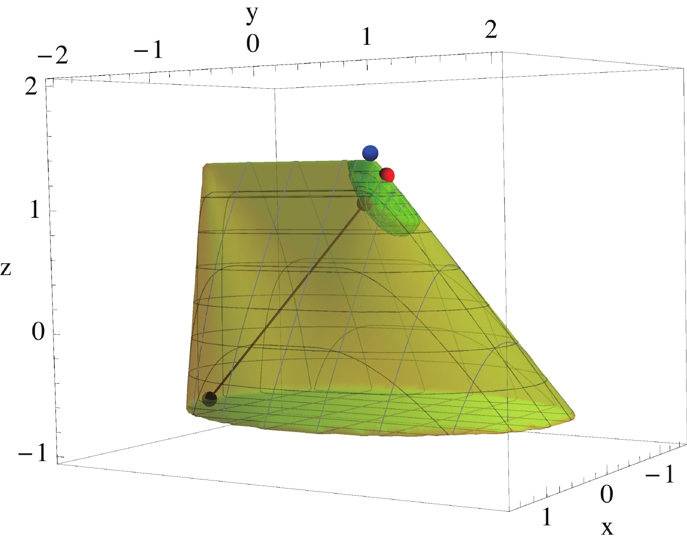
Figure 6. (color online) Three-dimensional cross section of the dimension-8 convex cone
$\cal C$ (yellow). This cross section is extracted as in Fig. 2. The experimental bounds, marginalized over the dimension-6 coefficients, are displayed by the green region. The blue, brown, red, and black dots represent the$\vec C^{(8)}_0$ ,$\vec C_{\rm{max}}^{(8)}$ ,$\vec C_{\rm{max}}^{(8)}-\lambda_{\rm{max}}\vec c_{V}^{\ (8)}$ , and$\vec c^{\ (8)}_{V}$ vectors, respectively. We refer to the text for more details.The black, brown, and red dots lie on a straight line, which stems from the fact that
$ \vec C_{\rm{max}}^{(8)} $ is a positively weighted sum of$ \vec C_{\rm{max}}^{(8)}-\lambda\vec c_{V}^{\ (8)} $ and$ \vec c_{V}^{\ (8)} $ . This figure further illustrates that the maximization process yielding the$ \lambda_{\rm{max}} $ quantity corresponds to estimating the largest possible distance between a point consistent with the experimental data and a point allowed by the positivity bounds in a given direction$ \vec c^{\ (8)}_{V} $ . Considering instead a$ \lambda $ value larger than$ \lambda_{\rm{max}} $ would mean to rely either on a setup experimentally excluded, or on a theory violating positivity. As these two options are evidently excluded,$ \lambda $ cannot be larger than$ \lambda_{\rm{max}} $ .The same class of universal bounds can be set on all types of potential states extending the SM in the UV. The Wilson coefficients relevant for our benchmark assumption
$ \vec C_0 $ of Eq. (45) are generated by integrating a scalar D-field out. However, the approach is most effective for all other particle types in Table 1. We present the results for the$ M_L $ ,$ M_R $ , V with$ \kappa = \pm1 $ (i.e., corresponding to a vector and axial-vector coupling to the electron field) and$ V' $ states in Table 4. This allows for the derivation, for each particle type, of the$ \lambda_{\max}\vec c^{\ (8)}_X $ quantity that depicts the maximum possible contribution from X-type particles to the generated dimension-8 operators$ \vec C_0^{(8)} = (0,0,0.04,0) $ . In most cases, bounds can be set at the 10%-20% level. This corresponds, after converting the results in terms of BSM scales, to roughly an exclusion of UV particles lighter than approximately$ 3-4 $ TeV.X $\vec{c}_{X}^{\ (8)}$ 

$\lambda_{\rm{max}}$ 

$M_X/\sqrt{g_X}$ 

$M_L$ 

$(0,0,0,-1)$ 

0.0067 $\geqslant 3.5$ TeV

$M_R$ 

$(-1,0,0,0)$ 

0.0069 $\geqslant 3.5$ TeV

V (with $\kappa=1$ )

$(-1/2,-1,0,-1/2)$ 

0.0055 $\geqslant 3.7$ TeV

V (with $\kappa=-1$ )

$(-1/2,1,0,-1/2)$ 

0.0116 $\geqslant 3.0$ TeV

$V'$ 

$(0,-1,2,0)$ 

0.0109 $\geqslant 3.1$ TeV

Table 4. Universal bounds imposed with positivity on the particle species X, and for a BSM setup in which the SM is extended by a D-type scalar. The bounds, expressed in terms of the
$\lambda_{\rm{max}}$ quantity of Eq. (50) (third column), are also translated in terms of the new physics masses and couplings (fourth column). We additionally recall the values of the different$\vec{c}_{X}^{\ (8)}$ vectors (second column).In contrast, for D-type scalars, we obtain a much larger
$ \lambda_{\max} $ value,$ \lambda_{\max}\approx 0.049\ . $

(52) Using Eq. (38), we could additionally infer a lower limit related to the existence of all types of particles. Such a limit is observed to be always 0, except for D-type particles for which we find
$ \lambda_{\rm{min}}\approx 0.011\ . $

(53) All these limits suggest that D-type particles should exist in viable UV completions, whereas all other types of particles are severely constrained. Such a result is not surprising and is consistent with our benchmark assumption. Such a conclusion thus provides the first steps to obtaining an answer to the “inverse problem”. We emphasize again that the obtained bounds are universal, in the sense that they apply without any assumption on the nature of the UV physics. Thus, they are useful to exclude BSM models and guide the model builders adopting a bottom-up approach.
Perhaps a more practically useful example in the light of the current LHC results is the SM case itself, where
$ \vec C_0 = 0 $ . In this context, the bounds on the dimension-6 Wilson coefficients are conventionally interpreted as bounds on the BSM mass scales and couplings, such as$ \frac{M_{D}}{g_{D}}\geqslant 16\;{\rm{TeV}}, \quad \frac{M_{M_L}}{g_{M_L}}\geqslant 17\;{\rm{TeV}} , \ \ldots $

(54) Whilst these are rather strong bounds, they can only be derived under very specific UV-model assumptions in which the SM is supplemented by a single heavy particle at a time. Therefore, they can easily be relaxed by considering more complicated models so that this one-particle interpretation is only useful for a top-down approach imposing a clear BSM setup in the UV. However, from the perspective of testing the SM, this is still insufficient, as one can never neither exclude the existence of any given class of BSM states, nor confirm the SM itself. There are indeed models whose dimension-6 coefficients feature cancellations or are suppressed for various reasons.
Dimension-8 positivity instead provides a chance to exclude the potential existence of any class of UV states universally in a bottom-up way, hence without any specific model assumptions. Focusing on the ILC-1000 collider, we extract bounds by using the same approach as in the previous example and present the results in Table 5, together with the model-dependent one-particle dimension-6 bounds. As expected, the universal bounds extracted from the positive nature of the dimension-8 coefficient parameter space are weaker than the one-particle dimension-6 bounds. However, they are still much higher than the collider energy of 1 TeV. Assuming that no deviations from the SM would be observed at the ILC-1000, these bounds will allow for the exclusion of any UV model featuring all types of states up to certain scales. In contrast to the dimension-6 case, it will not be possible to remove those constraints by adding or arranging the properties of other states, unless the latter is done in a way that violates the positivity bounds.
X $M_X/g_X$ 

$\lambda_{\rm{max}}$ 

$M_X/\sqrt{g_X}$ 

D $\geqslant 16$ TeV

0.0076 $\geqslant 3.4$ TeV

$M_L$ 

$\geqslant 17$ TeV

0.0053 $\geqslant 3.7$ TeV

$M_R$ 

$\geqslant 17$ TeV

0.0054 $\geqslant 3.7$ TeV

$V'$ 

$\geqslant 23$ TeV

0.0056 $\geqslant 3.7$ TeV

V (with $\kappa=1$ )

$\geqslant 28$ TeV

0.0041 $\geqslant 4.0$ TeV

V (with $\kappa=-1$ )

$\geqslant 21$ TeV

0.0041 $\geqslant 4.0$ TeV

Table 5. Bounds imposed on the existence of a particle species X, assuming the absence of BSM physics. The bounds are provided as limits on model-dependent one-particle extensions of the SM extracted from a fit of the dimension-6 coefficients (second column), as well as universal and model-independent bounds on a given particle species X derived from positivity. The latter are expressed in terms of the
$\lambda_{\rm{max}}$ quantity of Eq. (50) (third column) and in terms of the new physics masses and couplings (fourth column).In summary, studying dimension-8 operators in the context of future high-precision machines will pave the way for universal exclusions of entire classes of BSM theories by forbidding the existence of specific types of new states in the UV. Moreover, null BSM search results will eventually allow for the confirmation of the SM at scales much higher than the collider energies, providing the dimension-8 operators a special role in the precision test of the SM.
-
In this study, we have investigated the positivity features of the dimension-8 four-electron operators. We have, in particular, derived the complete set of positivity bounds for the
$ e^4D^2 $ class of operators using the elastic scatterings of states with arbitrary superpositions. Therefore, we have reproduced, by using a different approach, the results of Ref. [3], the latter having been derived using the extremal representation of dimension-8 positive convex cones. We have then investigated two phenomenological aspects of four-electron positivity at future lepton colliders.The first is the possibility of probing positivity violations, which, if present, will revolutionize our understanding of the fundamental pillars of QFT or the S-matrix theory. Practically, it would provide very important information for model building. We have proposed a model-independent quantification of the amount of violation and discussed the implications of positivity violations in terms of breaking the axiomatic properties of QFT and paving the way for non-standard UV completions of the SM. We have observed that positivity violation at scales of order 1–10 TeV can potentially be probed by all future lepton collider projects currently discussed within the high-energy physics community. This includes the CEPC, FCC-ee, ILC (with a possible energy upgrade), and CLIC colliders. At each collider, positivity violation effects can be probed up to scales of a factor of a few higher than the highest expected collider center-of-mass energy, regardless of the presence of any four-electron dimension-6 operators. This suggests an important and novel avenue for testing the fundamental principles of QFT at future lepton colliders. If their violation is observed, a more tailored description for the violated effect may be designed, and results could be improved through further model-specific studies.
The second aspect of our study is that, if the fundamental principles of QFT hold in the UV, the positive nature of the dimension-8 coefficient space allows us to infer the existence of new states at the UV scales directly and characterize their quantum numbers from measurements. Conversely, it allows for the exclusion of certain particles up to scales depending on the future measurement precision. This originates from several concepts in convex geometry and can be achieved without any BSM model assumption, in contrast to the conventional SMEFT interpretation truncated at the dimension-6 level that always requires a specific model assumption. Therefore, while a dimension-6-level approach is useful mostly for a top-down investigation of any given model, the dimension-8-level one is as important, as it provides the possibility of setting model-independent bounds on certain types of particles in the UV, or in other words, solving the inverse problem. We have demonstrated this point with realistic examples, using projected measurements at the ILC with an energy upgrade at 1 TeV. In particular, if no deviation from the SM is observed, we have explicitly shown how the existence of any type of heavy particles up to scales much higher than ILC energies can be excluded, regardless of the UV model setup, thanks to the requirement that any UV completion of the SM has to satisfy positivity. This underlines a major difference between dimension-6 and dimension-8 operators (or the s and
$ s^2 $ term in the amplitude). While one can design UV-complete models that result in vanishing dimension-6 operators due to accidental cancellations or for symmetry reasons (which makes it impossible to exclude reliably the presence of specific states in the UV), this does not hold at the dimension-8 level. By virtue of the positivity bounds, the dimension-8 operators are not allowed to vanish if the theory features extra states in the UV.Consequently, it is crucial to plan a comprehensive study of the dimension-8 operator effects, not only at the theoretical level but also at the experimental level.
Note added: After this paper appeared on the arXiv and was sent to Chin.Phys.C, Ref. [72] appeared on the arXiv. Its authors studied “explicit positivity bounds on dimension-six fermionic operators in the SMEFT.” Their results contrast with our observation in Section IV, where by explicitly integrating out all particle species in Table 1, we observed that any measured dimension-6 coefficient values could yield an infinite number of UV completions. Therefore, no bound exists. This difference from the results of Ref. [72] arises from neglecting the existence of new vector bosons in a UV completion.
-
We would like to thank Claudia de Rham, Andrew J. Tolley, and Alexander Vikman for useful comments on the manuscript. CZ would like to thank Jiayin Gu for helpful discussions related to collider analysis.
-
Here, we present details about how to obtain positivity bounds from the elastic scattering of two superposed states
$ f_1 $ and$ f_2 $ defined by$\tag{A1} f_{1,2}\equiv \epsilon_{1,2}^i F^i\ \ {\rm{with}}\ \ F^i\equiv \left( e_R,e_L,\nu_L,\bar e_R,\bar e_L,\bar \nu_L \right)\ , $

where
$ \epsilon_{1,2} $ are arbitrary complex six-vectors and the index i is summed over. We need to “scan” the full projective space of these vectors to exhaust all possible bounds and identify the most constraining ones.First, we show that mixings between fields with different chiralities do not provide any new bounds. To this end, we consider a forward scattering
$ f_1f_2\to f_1f_2 $ , where$ f_{1,2} $ consist of admixtures of left-handed fields$ f_L^i $ and right-handed fields$ f_R^i $ ,$\tag{A2} f_{1,2}\equiv a_{1,2}^i f_L^i + b_{1,2}^i f_R^i\ . $

The amplitude can be decomposed as
$\tag{A3} \begin{aligned}[b] M(f_1f_2\to f_1f_2) = & a^i_1a^{k\dagger}_1 a^j_2a^{l\dagger}_2 M(f_L^if_L^j \!\to\! f_L^kf_L^l) \!+\! b^i_1b^{k\dagger}_1 b^j_2b^{l\dagger}_2 M(f_R^if_R^j \!\to\! f_R^kf_R^l)\\ & + a^i_1a^{k\dagger}_1 b^j_2b^{l\dagger}_2 M(f_L^if_R^j \!\to\! f_L^kf_R^l) \!+\! b^i_1b^{k\dagger}_1 a^j_2a^{l\dagger}_2 M(f_R^if_L^j \!\to\! f_R^kf_L^l)\\ & + a^i_1b^{k\dagger}_1 a^j_2b^{l\dagger}_2 M(f_L^if_L^j \!\to\! f_R^kf_R^l) \!+\! b^i_1a^{k\dagger}_1 b^j_2a^{l\dagger}_2 M(f_R^if_R^j \!\to\! f_L^kf_L^l)\\ & + a^i_1b^{k\dagger}_1 b^j_2a^{l\dagger}_2 M(f_L^if_R^j \!\to\! f_R^kf_L^l) \!+\! b^i_1a^{k\dagger}_1 a^j_2b^{l\dagger}_2 M(f_R^if_L^j \!\to\! f_L^kf_R^l), \end{aligned} $

where once again, any repeated index is summed over. In this expression, the penultimate row vanishes because all the considered operators conserve chirality. Therefore, the involved fermions cannot flip chirality without a mass factor, and these contributions do not contribute to the positivity bounds obtained by performing a second-order s-derivative of the amplitude. Moreover, the last row vanishes because of the conservation of the angular momentum in the forward limit. Thus, only the first two rows are nonzero, and each remaining contribution is individually elastic. They can then be considered one by one, and they correspond to the four forward and elastic scattering matrix elements,
$\tag{A4} M(f_{1,R}f_{2,R} \to f_{1,R}f_{2,R}) , $

$\tag{A5} M(f_{1,L}f_{2,L} \to f_{1,L}f_{2,L}) , $

$\tag{A6} M(f_{1,R}f_{2,L} \to f_{1,R}f_{2,L}) , $

$\tag{A7} M(f_{1,L}f_{2,R} \to f_{1,L}f_{2,R}) , $

where
$ f_{n,L}\equiv a^n_1 f_L^i $ and$ f_{n,R}\equiv b^n_1 f_R^i $ ($ n = 1,2 $ ) represent the superpositions of left-handed fermions and right-handed fermions only, respectively. The positivity bounds are then fully encoded in the scattering amplitudes of these fields, which have a definite chirality. Such a feature is typical of four-fermion scattering in the SMEFT. In contrast, it does not hold for vector boson scattering, as there is no associated chirality conservation law in the SMEFT.To investigate the amplitudes in Eqs. (A4)–(A7), we utilize the crossing symmetry that shows that Eqs. (A4) and (A5), as well as Eqs. (A6) and (A7), are equal. Furthermore, Eqs. (A4) and (A6) are related by an
$ s\leftrightarrow u $ crossing,$\tag{A8} M(f_{1,R}f_{2,R} \to f_{1,R}f_{2,R}) = C_{s}s^2 + C_{t} t^2 + C_{u} u^2, $

$\tag{A9} M(f_{1,R}f_{2,L} \to f_{1,R}f_{2,L}) = C_{s}u^2 + C_{t} t^2 + C_{u} s^2, $

where
$ C_{s,t,u} $ denote generic coefficients. Since in the$ t\to 0 $ limit,$ u^2 = s^2 $ , all four amplitudes lead to the same positivity bound$ C_{s}+C_{u}>0 $ . Thus, it is sufficient to focus on only one of the four cases.Hence, we consider the
$ M(f_{1,R}f_{2,R} \to f_{1,R}f_{2,R}) $ amplitude. In the current problem, the right-handed$ f_R $ fields consist of mixtures of$ e_R $ ,$ \bar e_L $ , and$ \bar\nu_L $ ,$ \tag{A10} f_{n,R} = a_n e_R+b_n \bar e_L+c_n \bar\nu_L \quad{\rm{for}}\quad n = 1,2 , $

where
$ a_n,b_n,c_n $ are arbitrary complex numbers. Using the results presented in Appendix B, the second-order derivative of the amplitude w.r.t. s is determined to be$\tag{A11} \begin{aligned}[b] & \frac{1}{2}\frac{ {\rm{d}}^2}{ {\rm{d}} s^2}M(f_{1,R}f_{2,R} \to f_{1,R}f_{2,R}) = \\ &\qquad Af_A+Bf_B+Cf_C+Df_D+Ef_E , \end{aligned} $

where the quantities
$ f_A $ ,$ f_B $ ,$ f_C $ ,$ f_D $ , and$ f_E $ are given by$\tag{A12} \begin{aligned}[b] & f_A\! = \!-4C_1,\\& f_B\! = \!2C_2+C_3,\\&f_C\! = \!-4(C_4\!+\!C_5),\\ & f_D\! = \!-8C_5,\\& f_E\! = \!C_3, \end{aligned} $

and the parameters A, B, C, D, and E are
$\tag{A13} \begin{aligned}[b] & A = |a_1a_2^\dagger|^2, \\ & B = 2 \Re (a_1a_2^\dagger)(\vec x^\dagger\!\cdot\!\vec y),\\ & C = \left| \vec x \cdot \vec y^\dagger \right|^2, \\ & D = \left| \vec x \times \vec y \right|^2, \\& E = |a_1|^2\left|\vec y\right|^2 + |a_2|^2\left|\vec x\right|^2\ . \end{aligned} $

In these expressions, the vectors
$ \vec x $ and$ \vec y $ and their various dot and cross products are defined as$ \tag{A14}\begin{aligned}[b] & \vec x\equiv(b_1,c_1), \ \ \vec y\equiv(b_2,c_2),\\ & \vec u\cdot \vec v \equiv u_1v_1+u_2v_2,\ \ \vec u\times \vec v \equiv u_1v_2-u_2v_1\ . \end{aligned} $

The positivity bounds arise from the requirement that Eq. (A11) be positive for all possible values of the parameters A, B, C, D, and E . It can be observed that
$\tag{A15} A>0,\quad C>0,\quad D>0 . $

In addition,
$\tag{A16} |B| \! = \! 2 \left|\Re (a_1a_2^\dagger)\left( \vec x^\dagger\!\cdot\!\vec y \right)\right| \!<\! 2\left|a_1a_2^\dagger\right| \left|\vec x^\dagger\!\cdot\!\vec y \right| \! = \! 2\sqrt{AC}, $

and
$\tag{A17} E\! = \!|a_1|^2\left|\vec y\right|^2 \!+\! |a_2|^2\left|\vec x\right|^2 \!>\! 2|a_1|\left|\vec y\right| |a_2|\left|\vec x\right| \! = \! 2\sqrt{A(C+D)}, $

where we have used
$ C+D = \left|\vec x\right|^2\left|\vec y\right|^2 $ .We must then show that, for each set of parameters A, B, C, D, and E that satisfy the inequalities of Eqs. (A15)–(A17), there exists a corresponding set of coefficients
$ a_n $ ,$ b_n $ , and$ c_n $ . This is achieved by introducing$ \phi =$ $ \cos^{-1}\dfrac{B}{2\sqrt{AC}} $ and$ r>1 $ such that$ r^2+r^{-2} = E/\sqrt{A(C+D} $ . Then, at least the following values for$ a_n $ ,$ b_n $ , and$ c_n $ can be determined:$\tag{A18} \begin{aligned}[b] a_1 =& rA^{1/4}{\rm e}^{{\rm i}\phi},\\ a_2 =& r^{-1}A^{1/4},\\ (b_1,c_1) =& \sqrt[4]{C+D}(1,0),\\ (b_2,c_2) =& \sqrt[4]{C+D}\left( \frac{C^{1/2}}{(C+D)^{1/2}},\frac{D^{1/2}}{(C+D)^{1/2}}\right) . \end{aligned} $

Therefore, we conclude that the positivity bounds require that
$ \tag{A19} f\equiv Af_A+Bf_B+Cf_C+Df_D+Ef_E >0 , $

for any
$ A,B,C,D,E $ that are real and that satisfy$\tag{A20} \begin{aligned}[b]& A>0,\quad C>0, \quad D>0,\\ &-2\sqrt{AC}<B<2\sqrt{AC}, \\& 2\sqrt{A(C+D)}<E. \end{aligned} $

Equivalently, this implies that the function f has a minimum in the domain defined by Eq. (A20), and that this minimum is positive. The existence of a minimum implies that
$\tag{A21} f_D>0,\quad f_E>0 . $

Moreover, as
$ |B| $ has an upper bound and E has a lower bound, the minimum of f obtained by varying B and E is realized by$ B\to -{\rm{sign}}(f_B)2\sqrt{AC} $ and$ E\to$ $ 2\sqrt{A(C+D)} $ . In other words,$\tag{A22} \begin{aligned}[b] {f > {f_{BE}} \equiv} & {A{f_A} + C{f_C} - 2|{f_B}|\sqrt {AC} + D{f_D}}\\ &{ + 2\sqrt {A(C + D)} {f_E}.} \end{aligned} $

Since
$ f_D>0 $ , we could further decrease this function by taking$ D\to0 $ ,$ \tag{A23} f>f_{BED} = Af_A + 2(f_E-|f_B|)\sqrt{AC}+Cf_C . $

Finally, the minimal value of the above function has to be positive for any
$ A,C>0 $ , so that$\tag{A24} f_A>0,\; \; \; \; f_C>0, $

$ \tag{A25} f_E>|f_B|\quad{\rm{or}}\quad f_Af_C>(|f_B|-f_E)^2. $

The last of which is equivalent to
$ \tag{A26} \sqrt{f_Af_C}>f_B-f_E\quad{\rm{and}}\quad \sqrt{f_Af_C}>-f_B-f_E . $

Combining the inequalities of Eqs. (A21), (A24), and (A26) and plugging in the actual Wilson coefficients from Eq. (A12), we obtain the positivity bounds of Eqs. (7)–(12).
-
$ \begin{aligned} &M(e_Re_R\to e_Re_R) = -4 s^2 C_1 \\ &M(e_Re_L\to e_Re_L) = C_3 (s+t)^2+2 t C_2 (s+t) \\ &M(e_Re_L\to e_Le_R) = C_3 t^2+2 (s+t) C_2 t \\ &M(e_R\nu _L\to e_R\nu _L) = C_3 (s+t)^2+2 t C_2 (s+t) \\ \end{aligned} $

$\begin{aligned} &M(e_R\nu _L\to \nu _Le_R) = C_3 t^2+2 (s+t) C_2 t \\ &M(e_R\bar{e}_R\to e_R\bar{e}_R) = -4 (s+t)^2 C_1 \\ &M(e_R\bar{e}_R\to e_L\bar{e}_L) = t^2 C_3-2 s t C_2 \\ &M(e_R\bar{e}_R\to \nu _L\bar{\nu }_L) = t^2 C_3-2 s t C_2 \\ &M(e_R\bar{e}_R\to \bar{e}_Re_R) = -4 t^2 C_1 \\ &M(e_R\bar{e}_R\to \bar{e}_Le_L) = C_3 (s+t)^2+2 s C_2 (s+t) \\ &M(e_R\bar{e}_R\to \bar{\nu }_L\nu _L) = C_3 (s+t)^2+2 s C_2 (s+t) \\ &M(e_R\bar{e}_L\to e_R\bar{e}_L) = s^2 C_3-2 s t C_2 \\ &M(e_R\bar{e}_L\to \bar{e}_Le_R) = C_3 s^2+2 (s+t) C_2 s \\ &M(e_R\bar{\nu }_L\to e_R\bar{\nu }_L) = s^2 C_3-2 s t C_2 \\ &M(e_R\bar{\nu }_L\to \bar{\nu }_Le_R) = C_3 s^2+2 (s+t) C_2 s \\ &M(e_Le_R\to e_Re_L) = C_3 t^2+2 (s+t) C_2 t \\ &M(e_Le_R\to e_Le_R) = C_3 (s+t)^2+2 t C_2 (s+t) \\ &M(e_Le_L\to e_Le_L) = -4 C_4 s^2-4 C_5 s^2 \\ &M(e_L\nu _L\to e_L\nu _L) = 4 s t C_4-4 s (2 s+3 t) C_5 \\ &M(e_L\nu _L\to \nu _Le_L) = 4 s (s+3 t) C_5-4 s (s+t) C_4 \\ &M(e_L\bar{e}_R\to e_L\bar{e}_R) = s^2 C_3-2 s t C_2 \\ &M(e_L\bar{e}_R\to \bar{e}_Re_L) = C_3 s^2+2 (s+t) C_2 s \\ &M(e_L\bar{e}_L\to e_R\bar{e}_R) = t^2 C_3-2 s t C_2 \\ &M(e_L\bar{e}_L\to e_L\bar{e}_L) = -4 C_4 (s+t)^2-4 C_5 (s+t)^2 \\ &M(e_L\bar{e}_L\to \nu _L\bar{\nu }_L) = 4 (s-2 t) (s+t) C_5-4 s (s+t) C_4 \\ &M(e_L\bar{e}_L\to \bar{e}_Re_R) = C_3 (s+t)^2+2 s C_2 (s+t) \\ &M(e_L\bar{e}_L\to \bar{e}_Le_L) = -4 C_4 t^2-4 C_5 t^2 \\ &M(e_L\bar{e}_L\to \bar{\nu }_L\nu _L) = 4 s t C_4-4 t (3 s+2 t) C_5 \\ &M(e_L\bar{\nu }_L\to e_L\bar{\nu }_L) = -4 t (s+t) C_4-4 (2 s-t) (s+t) C_5 \\ &M(e_L\bar{\nu }_L\to \bar{\nu }_Le_L) = 4 t (3 s+t) C_5-4 t (s+t) C_4 \\ &M(\nu _Le_R\to e_R\nu _L) = C_3 t^2+2 (s+t) C_2 t \\ &M(\nu _Le_R\to \nu _Le_R) = C_3 (s+t)^2+2 t C_2 (s+t) \\ &M(\nu _Le_L\to e_L\nu _L) = 4 s (s+3 t) C_5-4 s (s+t) C_4 \\ &M(\nu _Le_L\to \nu _Le_L) = 4 s t C_4-4 s (2 s+3 t) C_5 \\ &M(\nu _L\nu _L\to \nu _L\nu _L) = -4 C_4 s^2-4 C_5 s^2 \\ &M(\nu _L\bar{e}_R\to \nu _L\bar{e}_R) = s^2 C_3-2 s t C_2 \\ &M(\nu _L\bar{e}_R\to \bar{e}_R\nu _L) = C_3 s^2+2 (s+t) C_2 s \\ &M(\nu _L\bar{e}_L\to \nu _L\bar{e}_L) = -4 t (s+t) C_4-4 (2 s-t) (s+t) C_5 \\ &M(\nu _L\bar{e}_L\to \bar{e}_L\nu _L) = 4 t (3 s+t) C_5-4 t (s+t) C_4 \\ &M(\nu _L\bar{\nu }_L\to e_R\bar{e}_R) = t^2 C_3-2 s t C_2 \\ &M(\nu _L\bar{\nu }_L\to e_L\bar{e}_L) = 4 (s-2 t) (s+t) C_5-4 s (s+t) C_4 \\ &M(\nu _L\bar{\nu }_L\to \nu _L\bar{\nu }_L) = -4 C_4 (s+t)^2-4 C_5 (s+t)^2 \\ &M(\nu _L\bar{\nu }_L\to \bar{e}_Re_R) = C_3 (s+t)^2+2 s C_2 (s+t) \\ &M(\nu _L\bar{\nu }_L\to \bar{e}_Le_L) = 4 s t C_4-4 t (3 s+2 t) C_5 \\ &M(\nu _L\bar{\nu }_L\to \bar{\nu }_L\nu _L) = -4 C_4 t^2-4 C_5 t^2 \\ \end{aligned} $

$ \begin{aligned} &M(\bar{e}_Re_R\to e_R\bar{e}_R) = -4 t^2 C_1 \\ &M(\bar{e}_Re_R\to e_L\bar{e}_L) = C_3 (s+t)^2+2 s C_2 (s+t) \\ &M(\bar{e}_Re_R\to \nu _L\bar{\nu }_L) = C_3 (s+t)^2+2 s C_2 (s+t) \\ &M(\bar{e}_Re_R\to \bar{e}_Re_R) = -4 (s+t)^2 C_1 \\ &M(\bar{e}_Re_R\to \bar{e}_Le_L) = t^2 C_3-2 s t C_2 \\ &M(\bar{e}_Re_R\to \bar{\nu }_L\nu _L) = t^2 C_3-2 s t C_2 \\ &M(\bar{e}_Re_L\to e_L\bar{e}_R) = C_3 s^2+2 (s+t) C_2 s \\ &M(\bar{e}_Re_L\to \bar{e}_Re_L) = s^2 C_3-2 s t C_2 \\ &M(\bar{e}_R\nu _L\to \nu _L\bar{e}_R) = C_3 s^2+2 (s+t) C_2 s \\ &M(\bar{e}_R\nu _L\to \bar{e}_R\nu _L) = s^2 C_3-2 s t C_2 \\ &M(\bar{e}_R\bar{e}_R\to \bar{e}_R\bar{e}_R) = -4 s^2 C_1 \\ &M(\bar{e}_R\bar{e}_L\to \bar{e}_R\bar{e}_L) = C_3 (s+t)^2+2 t C_2 (s+t) \\ &M(\bar{e}_R\bar{e}_L\to \bar{e}_L\bar{e}_R) = C_3 t^2+2 (s+t) C_2 t \\ &M(\bar{e}_R\bar{\nu }_L\to \bar{e}_R\bar{\nu }_L) = C_3 (s+t)^2+2 t C_2 (s+t) \\ &M(\bar{e}_R\bar{\nu }_L\to \bar{\nu }_L\bar{e}_R) = C_3 t^2+2 (s+t) C_2 t \\ &M(\bar{e}_Le_R\to e_R\bar{e}_L) = C_3 s^2+2 (s+t) C_2 s \\ &M(\bar{e}_Le_R\to \bar{e}_Le_R) = s^2 C_3-2 s t C_2 \\ &M(\bar{e}_Le_L\to e_R\bar{e}_R) = C_3 (s+t)^2+2 s C_2 (s+t) \\ &M(\bar{e}_Le_L\to e_L\bar{e}_L) = -4 C_4 t^2-4 C_5 t^2 \\ &M(\bar{e}_Le_L\to \nu _L\bar{\nu }_L) = 4 s t C_4-4 t (3 s+2 t) C_5 \\ &M(\bar{e}_Le_L\to \bar{e}_Re_R) = t^2 C_3-2 s t C_2 \\ &M(\bar{e}_Le_L\to \bar{e}_Le_L) = -4 C_4 (s+t)^2-4 C_5 (s+t)^2 \\ \end{aligned} $

$\tag{B1} \begin{aligned} &M(\bar{e}_Le_L\to \bar{\nu }_L\nu _L) = 4 (s-2 t) (s+t) C_5-4 s (s+t) C_4 \\ &M(\bar{e}_L\nu _L\to \nu _L\bar{e}_L) = 4 t (3 s+t) C_5-4 t (s+t) C_4 \\ &M(\bar{e}_L\nu _L\to \bar{e}_L\nu _L) = -4 t (s+t) C_4-4 (2 s-t) (s+t) C_5 \\ &M(\bar{e}_L\bar{e}_R\to \bar{e}_R\bar{e}_L) = C_3 t^2+2 (s+t) C_2 t \\ &M(\bar{e}_L\bar{e}_R\to \bar{e}_L\bar{e}_R) = C_3 (s+t)^2+2 t C_2 (s+t) \\ &M(\bar{e}_L\bar{e}_L\to \bar{e}_L\bar{e}_L) = -4 C_4 s^2-4 C_5 s^2 \\ &M(\bar{e}_L\bar{\nu }_L\to \bar{e}_L\bar{\nu }_L) = 4 s t C_4-4 s (2 s+3 t) C_5 \\ &M(\bar{e}_L\bar{\nu }_L\to \bar{\nu }_L\bar{e}_L) = 4 s (s+3 t) C_5-4 s (s+t) C_4 \\ &M(\bar{\nu }_Le_R\to e_R\bar{\nu }_L) = C_3 s^2+2 (s+t) C_2 s \\ &M(\bar{\nu }_Le_R\to \bar{\nu }_Le_R) = s^2 C_3-2 s t C_2 \\ &M(\bar{\nu }_Le_L\to e_L\bar{\nu }_L) = 4 t (3 s+t) C_5-4 t (s+t) C_4 \\ &M(\bar{\nu }_Le_L\to \bar{\nu }_Le_L) = -4 t (s+t) C_4-4 (2 s-t) (s+t) C_5 \\ &M(\bar{\nu }_L\nu _L\to e_R\bar{e}_R) = C_3 (s+t)^2+2 s C_2 (s+t) \\ &M(\bar{\nu }_L\nu _L\to e_L\bar{e}_L) = 4 s t C_4-4 t (3 s+2 t) C_5 \\ &M(\bar{\nu }_L\nu _L\to \nu _L\bar{\nu }_L) = -4 C_4 t^2-4 C_5 t^2 \\ &M(\bar{\nu }_L\nu _L\to \bar{e}_Re_R) = t^2 C_3-2 s t C_2 \\ &M(\bar{\nu }_L\nu _L\to \bar{e}_Le_L) = 4 (s-2 t) (s+t) C_5-4 s (s+t) C_4 \\ &M(\bar{\nu }_L\nu _L\to \bar{\nu }_L\nu _L) = -4 C_4 (s+t)^2-4 C_5 (s+t)^2 \\ &M(\bar{\nu }_L\bar{e}_R\to \bar{e}_R\bar{\nu }_L) = C_3 t^2+2 (s+t) C_2 t \\ &M(\bar{\nu }_L\bar{e}_R\to \bar{\nu }_L\bar{e}_R) = C_3 (s+t)^2+2 t C_2 (s+t) \\ &M(\bar{\nu }_L\bar{e}_L\to \bar{e}_L\bar{\nu }_L) = 4 s (s+3 t) C_5-4 s (s+t) C_4 \\ &M(\bar{\nu }_L\bar{e}_L\to \bar{\nu }_L\bar{e}_L) = 4 s t C_4-4 s (2 s+3 t) C_5 \\ &M(\bar{\nu }_L\bar{\nu }_L\to \bar{\nu }_L\bar{\nu }_L) = -4 C_4 s^2-4 C_5 s^2 \end{aligned} $

Positivity in electron-positron scattering: testing the axiomatic quantum field theory principles and probing the existence of UV states
- Received Date: 2020-09-07
- Available Online: 2021-02-15
Abstract: We consider the positivity bounds on dimension-8 four-electron operators and study two related phenomenological aspects at future lepton colliders. First, if positivity is violated, probing such violations will revolutionize our understanding of the fundamental pillars of quantum field theory and the S-matrix theory. We observe that positivity violation at scales of 1-10 TeV can potentially be probed at future lepton colliders even if one assumes that dimension-6 operators are also present. Second, the positive nature of the dimension-8 parameter space often allows us to either directly infer the existence of UV-scale particles together with their quantum numbers or exclude them up to certain scales in a model-independent way. In particular, dimension-8 positivity plays an important role in the test of the Standard Model. If no deviations from the Standard Model are observed, it allows for simultaneous exclusion limits on all kinds of potential UV-complete models. Unlike the dimension-6 case, these limits apply regardless of the UV model setup and cannot be removed by possible cancellations among various UV contributions. This thus consists of a novel and universal test to confirm the Standard Model. We demonstrate with realistic examples how all the previously mentioned possibilities, including the test of positivity violation, can be achieved. Hence, we provide an important motivation for studying dimension-8 operators more comprehensively.


 DownLoad: