


 Abstract
 HTML
HTML Reference
 Related
 PDF
PDF


-
In the 1930s, Zwicky [1] and Smith [2] found that the velocity dispersion of galaxies in clusters is so high that the galaxies cannot be bounded to the cluster just by the gravitational force generated by visible matter. Hence it was concluded that there must be a large amount of invisible matter in cluster, which is now called dark matter (DM). Decades later, Rubin and his collaborators [3-5] found strong evidence for the existence of DM from the observations of galaxy rotation curves. Other observational evidence for the existence of DM includes the strong and weak gravitational lensing of Bullet Cluster 1E 0657-558 [6], the observation of cosmic microwave background radiation from the Planck satellite [7], the excess of positron abundance in cosmic rays [8], and so on. In recent decades, extensive searches have been made for DM particles, but have not yet been successful [9]. Meanwhile, various alternative models have been proposed to explain the extra gravitational force generated by DM, such as the modified Newtonian dynamics (MOND) model [10-12] and modified gravity models [13-15].
The MOND theory was originally proposed to account for the rotation curves of spiral galaxies, see e.g. Refs. [16, 17] for a recent review. According to MOND, Newton's second law loses its efficacy if the acceleration is below a critical value
$ a_{0} $ . MOND theory has achieved great success in interpreting the rotation curves of spiral galaxies [18-26]. For a long time, MOND was a non-relativistic theory, until Bekenstein [27] constructed its relativistic form. The relativistic form of MOND, i.e. the tensor-vector-scalar (TeVeS) theory [27, 28], has been discussed in the weak field regime, and tested in the Solar system [29, 30]. Moreover, MOND is consistent with the baryonic Tully-Fisher relation observed in spiral galaxies [31]. MOND theory introduces a free parameter$ a_0 $ , a characteristic acceleration scale below which Newtonian dynamics breaks down. If MOND theory is a fundamental theory,$ a_0 $ must be a universal constant.To study the characteristic acceleration of MOND theory, we need to match the theory with observations. Recently, the Spitzer Photometry and Accurate Rotation Curves (SPARC) database [32] has been released. It is extensively used to investigate the radial acceleration relation [33-35]. Based on the SPARC data, some debates on MOND as a fundamental theory have attracted extensive attention [36-38]. Using Bayesian inference with flat priors, Rodrigues et al. [37] concluded that MOND was excluded as a fundamental theory at more than
$ 10\sigma $ based on 193 high-quality disk galaxies from the SPARC and The HI Nearby Galaxy Survey (THINGS) databases. Later on, Chang et al. [38] fitted the rotation curves of 175 SPARC galaxies using a similar method but with Gaussian priors, and came to the similar conclusion that MOND theory cannot hold as a fundamental theory. As the representative and currently largest collection of rotating curved galaxies, SPARC data contains galaxies of different morphological types, luminosity and effective surface brightness. In the previous works [33-38], the qualified SPARC data was used as a whole. It is meaningful to test if the acceleration scale is dependent on the galaxy morphological types or not. In our work, we will classify the SPARC dataset depending on the galaxy morphological types, and test the possible galaxy-dependence of the characteristic acceleration scale.The original MOND theory [10-12] only requires two limit conditions. One is the Newtonian region, that is, Newton's second law should be valid while
$ a_0\rightarrow0 $ . The other is the deep MOND region, that is, Newton's second law should be modified to satisfy the Tully-Fisher relation [39]. To match the MOND theory with astronomical observations, an interpolation function is needed. If MOND theory is a fundamental theory, the acceleration scale$ a_0 $ should not depend on the specific choice of interpolation function. In this paper, we will consider five popular interpolation functions to match the SPARC data.It has been noted that the best-fit value
$ a_0\sim1.2\times10^{-10}\; m/s^2 $ , obtained from fitting to a large sample of spiral galaxies, is numerically close to$ cH_{0}/2\pi $ [40], where c is the speed of light and$ H_0 $ is the Hubble constant [10]. It is unclear if this correlation has some physical implications or is just a coincidence. If the former is true, then$ a_0 $ must be correlated with the evolution history of the universe. Some astronomical and cosmological observations, such as the luminosity of type-Ia supernovae [41], the spatial variation of the fine-structure constant [42], the cosmic microwave background radiation [43, 44], etc., show that the universe may be anisotropic. Hence it is necessary to investigate if the acceleration scale$ a_0 $ is directionally dependent or not. In fact, Zhou et al. [45] have already studied the possible anisotropy of$ a_0 $ using the SPARC data, and found that the direction of maximum anisotropy is close to the direction of the “Australia dipole” for the fine-structure constant. In their following work, Chang et al. [46] studied a dipole correction for$ a_0 $ , and found a similar dipole direction. Inspired by this, here we continue to investigate the possible anisotropy of the acceleration scale. We will focus on testing if different interpolation functions have some influence on the anisotropy.The rest of this paper is organized as follows. In Sec. II, we briefly review the MOND theory and some commonly discussed interpolation functions, and introduce the SPARC data set used in our studies. In Sec. III, we fit the SPARC data to the MOND theory, taking into account five different interpolation functions and different galaxy types, as well as the sky direction of the galaxies. Finally, a short summary is given in Sec. IV.
-
The MOND theory [10, 11] was initially proposed by Milgrom to account for the missing-mass problem in rotationally supported galaxies, to avoid having to introduce exotic dark matter. The main idea of MOND is that there is a critical acceleration
$ a_0 $ below which Newton's second laws are no longer valid (the MOND region), while above$ a_0 $ Newton's second law still holds (the Newtonian region). An interpolation function$ \mu(x) $ is used to join these two regions. Phenomenologically, the dynamics in MOND theory can be written as$ \mu\left(\frac{g}{a_{0}}\right)g = g_{\rm N}, $

(1) where
$ {g}_{\rm N}\equiv GM/r^{2} $ is the Newtonian acceleration,$ a_{0} $ is the critical acceleration, and$ \mu(x) $ is a smooth and monotonically increasing function of x. To be in accordance with the asymptotically flat feature of the observed galaxy rotation curves,$ \mu(x) $ must satisfy the asymptotic condition$ \mu(x)\approx x $ when$ x\rightarrow0 $ . To recover Newtonian dynamics,$ \mu(x) $ should be equal to unity when$ x\rightarrow\infty $ . In the deep-MOND limit, namely,$ g\ll a_{0} $ , the effective acceleration becomes$ g = \sqrt{a_{0}g_{\rm N}} $ .Given the matter distribution in a galaxy, it is easy to calculate the Newtonian acceleration
$ g_{\rm N} $ by solving the Poisson equation, and then the MOND acceleration g can be solved from Eq. (1). It is convenient to rewrite Eq. (1) in the following form:$ \nu\left(\frac{g_{\rm N}}{a_{0}}\right)g_{\rm N} = g. $

(2) Note that
$ y\nu(y) $ is the inverse of$ x\mu(x) $ , and it satisfies$ \nu(y)\approx1 $ when$ y\rightarrow\infty $ , and$ \nu(y)\approx y^{-1/2} $ when$ y\rightarrow0 $ . To fit the observations to the theoretical predictions, it is necessary to clarify the form of interpolation function$ \mu(x) $ or$ \nu(y) $ . However, the MOND theory does not give any hints on the concrete form of the interpolation function. Any smooth and monotonic function satisfying the above asymptotic conditions could be chosen. In general, there are two families of interpolation functions, namely, the$ \mu $ -function family and the$ \nu $ -function family. Any$ \mu $ -function has a corresponding$ \nu $ -function, although in some cases it is not easy to find an analytical expression. Different forms of interpolation functions have been discussed in Ref. [16]. In our work, five common interpolation functions are considered, including four$ \mu $ -functions and one$ \nu $ -function.The first interpolation function is the so-called “standard” function initially proposed by Milgrom [11], which takes the form:
$ \mu_{\rm{sta}}(x) = \frac{x}{\sqrt{1+x^{2}}}. $

(3) This function was widely used to analyse the galaxy rotation curves at the beginning of MOND theory [18, 19]. However, Famaey et al. [20] found that the “simple” function, another widely used interpolation function, gives a better fit to the terminal velocity curve of the Milky Way than the “standard” function. The "simple" function is:
$ \mu_{\rm{sim}}(x) = \frac{x}{1+x}. $

(4) Some studies show that this “simple” function performs better than the “standard” function in some cases [22, 47].
The initial MOND is a phenomenological model and is non-relativistic. Bekenstein [27] constructed a relativistic form, namely, the TeVeS theory. There is still a freedom in choosing the specific form of the scalar field action in TeVeS theory. The scalar action proposed in Ref. [27] gives rise to the following “toy” interpolation function,
$ \mu_{\rm{toy}}(x) = \frac{\sqrt{1+4x}-1}{\sqrt{1+4x}+1}. $

(5) This interpolation function gives a much slower transition from the MOND region to the Newtonian region than the “standard” and “simple” functions. The Finslerian model proposed in Ref. [48] also leads to the “toy” interpolation function.
The fourth interpolation function we consider is the so-called “exponential” function [11], which reads:
$ \mu_{\rm{exp}}(x) = 1-{\rm e}^{-x}. $

(6) This interpolation function behaves similarly to the “standard” function.
Finally, we also consider a
$ \nu $ -function, which is inspired by the radial acceleration relation (RAR) found from the SPARC data by Ref. [33]. It takes the form:$ \nu_{\rm{rar}}(y) = \frac{1}{1-{\rm e}^{-\sqrt{y}}}. $

(7) It has been shown that this
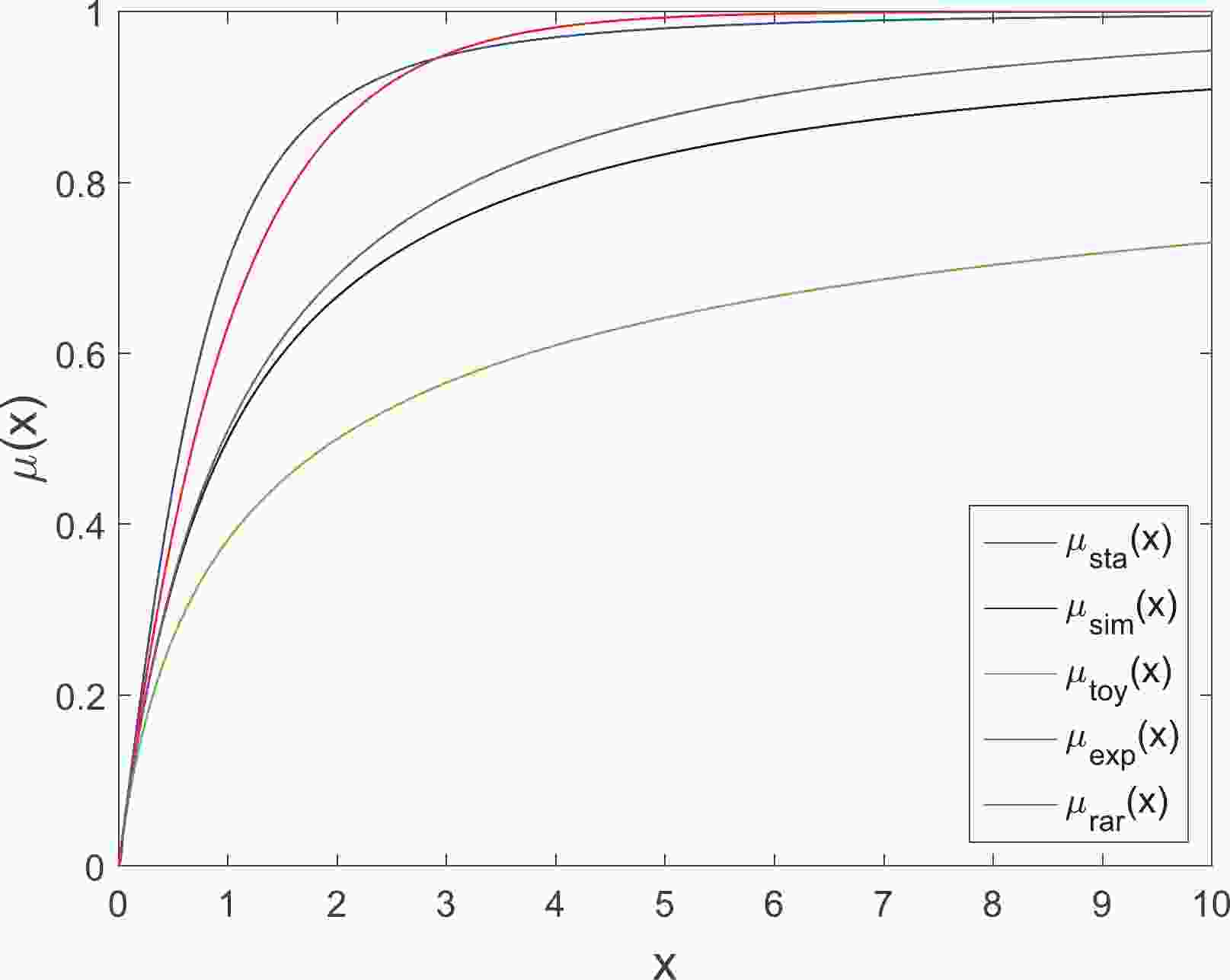
$ \nu $ -function can give a good fit to the rotation curves of the Milky Way [24]. Recently, this function has been used by McGaugh to fit the radial acceleration relation observed from a large sample of rotationally supported galaxies [33]. The$ \mu $ -function corresponding to this$ \nu $ -function can be obtained numerically, and is plotted, together with the other four$ \mu $ -functions, in Fig. 1. The “standard” and “exponential” functions show a sharp jump from the MOND region to the Newtonian region, while the “toy” function changes slowly, and the “simple” and “RAR” functions fall in between.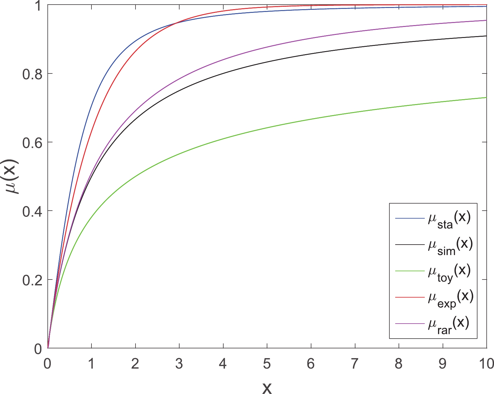
Figure 1. (color online) Plot of different interpolation functions.
To investigate the universality of the acceleration scale, we fit the above five functions with the recently released SPARC dataset [32]. This sample contains 175 disk galaxies with high quality observations at near-infrared (3.6 μm) and 21 cm, so both the baryon distribution and velocity field can be obtained. This dataset has already been used to study the radial acceleration relation [33, 34], i.e. the relation between the observed acceleration (
$ g_{\rm{obs}} $ ) and that expected from the baryonic matter ($ g_{\rm{bar}} $ , which is equivalent to$ g_{\rm N} $ in Eq. (1)) in the framework of Newtonian dynamics. In our work, the same selection criteria are adopted as Refs. [33, 34]: the 12 objects with asymmetric rotation curves which do not trace the equilibrium gravitational potential (quality flag Q = 3) and 10 face-on galaxies with$ i<30^{\circ} $ have been excluded, which leaves a sample of 153 galaxies. Furthermore, the condition that the relative uncertainty of the observed velocity ($ \delta V_{\rm obs}/V_{\rm obs} $ ) should be less than 10% has been applied. Therefore, the final data set used in our work contains 2693 data points in 147 galaxies.To fit theoretical predictions with the observational data, the orthogonal-distance-regression algorithm [49, 50] is adopted, which considers errors on both the horizontal and vertical axes. The best-fit parameters are obtained by minimizing the following
$ \chi^{2} $ :$ \chi^{2} = \sum\limits_{i = 1}^{N}\frac{[g_{\rm th}(g_{{\rm bar},i}+\delta_{i})-g_{{\rm obs},i}]^{2}}{\sigma_{{\rm obs},i}^{2}}+\frac{\delta_{i}^{2}}{\sigma_{{\rm bar},i}^{2}}, $

(8) where
$ g_{\rm obs} $ is the observed acceleration,$ g_{\rm bar} $ is the acceleration contributed by the baryonic matter, calculated in the framework of Newtonian dynamics,$ g_{\rm th} $ is the theoretical acceleration predicted by MOND, and$ \sigma_{\rm obs} $ and$ \sigma_{\rm bar} $ are the uncertainty of$ g_{\rm obs} $ and$ g_{\rm bar} $ , respectively.$ \delta $ is an auxiliary parameter for determining the weighted orthogonal (shortest) distance from the best-fit curve, which can be obtained interactively in the fitting procedure. The only free parameter is the acceleration scale$ a_0 $ . -
The SPARC data used here contains 147 galaxies of different Hubble types. Most of them are spiral galaxies from Sa to Sm. It also includes some lenticular galaxies (S0), irregular galaxies (Im) and blue compact dwarf galaxies (BCD). To study the possible dependence of
$ a_0 $ on the galaxy morphology, we classify the SPARC data set into several subsets according to the galaxy Hubble types. The Hubble types of the galaxies are labelled from 0 to 11: 0 = S0, 1 = Sa, 2 = Sab, 3 = Sb, 4 = Sbc, 5 = Sc, 6 = Scd, 7 = Sd, 8 = Sdm, 9 = Sm, 10 = Im, 11 = BCD. The number of galaxies in each Hubble type is shown in the histogram in Fig. 2. First, we divide the galaxies into two subsets: the spiral galaxies (from 1 to 9; denoted "Spiral" below) and the other galaxies (including 0, 10 and 11; denoted "Other" below). There are 2433 data points in 118 Spiral galaxies and 260 data points in 29 Other galaxies. Due to the significant difference in the number of data points between Spiral and Other galaxies, we further divide the Spiral galaxies into two subsets, with an approximately equal number of data points in each subset: Spiral-1 galaxies (from 1 to 4) and Spiral-2 galaxies (from 5 to 9). There are 1201 data points in 41 Spiral-1 galaxies and 1232 data points in 77 Spiral-2 galaxies. The details of the galaxy classification are shown in Table 1.Full Spiral Other Spiral-1 Spiral-2 Hubble type 0-11 1-9 0,10,11 1-4 5-9 Number of galaxies 147 118 29 41 77 Number of data points 2693 2433 260 1201 1232 Table 1. Details of galaxy classification.

Figure 2. Number of galaxies in each Hubble type.
First, we use the full dataset (denoted "Full") containing 2693 data points to fit the MOND theory with different interpolation functions. The best-fit
$ a_0 $ values are listed in Table 2, and the corresponding fitting curves between the Newtonian acceleration$ g_{\rm N} $ and the MOND acceleration g are shown in Fig. 3(a). We can see that the best-fit$ a_0 $ varies between different interpolation functions. The “toy” function seems to have the smallest$ \chi^2 $ , but this function also leads to the smallest$ a_{0} $ . This is because the “toy” function evolves much more slowly than the other four functions, as can be seen in Fig. 1. The “standard” function has the largest$ a_0 $ , but also has the largest$ \chi^2 $ , since this function shows the sharpest jump from the MOND region to the Newtonian region. The$ a_0 $ values from the “simple” and “RAR-inspired” functions are close to each other, because of their similar evolution behaviours.$\mu_{\rm{sta}}(x)$ 

$\mu_{\rm{sim}}(x)$ 

$\mu_{\rm{toy}}(x)$ 

$\mu_{\rm{exp}}(x)$ 

$\nu_{\rm{rar}}(y)$ 

Full $a_{0}$ 

$1.39\pm0.02$ 

$1.00\pm0.01$ 

$0.69\pm0.01$ 

$1.24\pm0.02$ 

$1.02\pm0.02$ 

$\chi^{2}/dof$ 

$1.73$ 

$1.48$ 

$1.47$ 

$1.66$ 

$1.49$ 

Spiral $a_{0}$ 

$1.50\pm0.02$ 

$1.07\pm0.02$ 

$0.73\pm0.01$ 

$1.34\pm0.04$ 

$1.09\pm0.02$ 

$\chi^{2}/dof$ 

$1.46$ 

$1.26$ 

$1.28$ 

$1.39$ 

$1.27$ 

Other $a_{0}$ 

$0.86\pm0.04$ 

$0.70\pm0.04$ 

$0.55\pm0.04$ 

$0.79\pm0.04$ 

$0.71\pm0.04$ 

$\chi^{2}/dof$ 

$3.06$ 

$2.99$ 

$3.00$ 

$3.08$ 

$3.01$ 

Spiral-1 $a_{0}$ 

$1.70\pm0.03$ 

$1.08\pm0.03$ 

$0.61\pm0.02$ 

$1.48\pm0.03$ 

$1.12\pm0.03$ 

$\chi^{2}/dof$ 

$1.14$ 

$0.986$ 

$1.04$ 

$1.10$ 

$0.99$ 

Spiral-2 $a_{0}$ 

$1.43\pm0.02$ 

$1.06\pm0.02$ 

$0.78\pm0.02$ 

$1.28\pm0.02$ 

$1.08\pm0.02$ 

$\chi^{2}/dof$ 

$1.73$ 

$1.52$ 

$1.48$ 

$1.65$ 

$1.53$ 

Table 2. Best-fit
$a_0$ values for five different interpolation functions and different datasets. The unit of$a_{0}$ is$10^{-10}$ m s$^{-2}$ .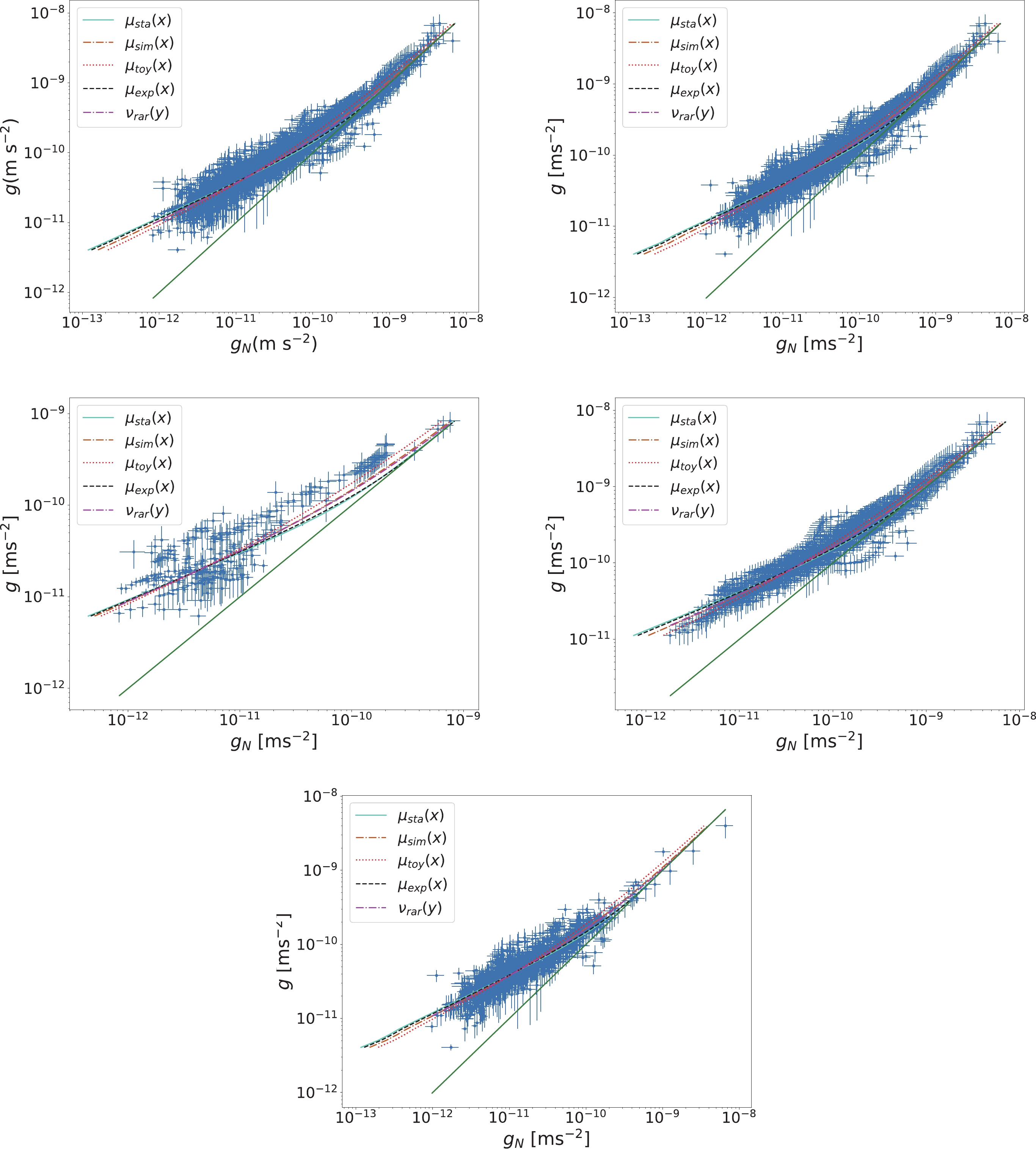
Figure 3. (color online) Best-fit curves of the radial acceleration relation. The observational data points are shown by blue dots with error bars. The green solid line is the line of unity.
Then, we divide the Full sample into the Spiral and Other subsamples, and fit each subsample to the MOND theory. The best-fit results are reported in Table 2, and the best-fit curves are plotted in Figs. 3(b) and 3(c), respectively. For both subsamples, the “simple” function has the smallest
$ \chi^2 $ , but the best-fit$ a_0 $ differs significantly, namely,$ a_{0} = (1.07\pm0.02)\times10^{-10} $ ms$ ^{-2} $ for the Spiral sample and$ a_{0} = (0.70\pm0.04)\times10^{-10} $ ms$ ^{-2} $ for the Other sample. For a fixed interpolation function, the Other sample has a much smaller$ a_0 $ than the Spiral sample, and$ a_0 $ of the Full sample falls in between. This implies that the Spiral galaxies and Other galaxies have very different$ a_0 $ . For both the Spiral and Other subsamples, the best-fitting$ a_0 $ is also dependent on the choice of interpolation function.Finally, we further divide the Spiral sample into the two subsamples denoted by Spiral-1 and Spiral-2, and use these two subsamples to fit to the MOND theory. The best-fit parameters are presented in the last four rows in Table 2, and the best-fit curves are plotted in Figs. 3(d) and 3(e), respectively. The “simple” function is the best for the Spiral-1 subsample, with the best-fit value
$ a_{0} = (1.08\pm0.03)\times10^{-10} $ ms$ ^{-2} $ . For the Spiral-2 subsample, the “toy” function fits the data best, with the best-fit value$ a_{0} = (0.78\pm0.02)\times10^{-10} $ ms$ ^{-2} $ . Similarly, for a fixed interpolation function, the Spiral-1 and Spiral-2 subsamples may lead to different values of$ a_{0} $ , but the difference seems to be not as significant as that between the Spiral and Other subsamples. Especially, for the “simple” and “RAR-inspired” functions, the values of$ a_{0} $ for the Spiral-1 and Spiral-2 subsamples are consistent with each other within$ 1\sigma $ uncertainty.As a summary, we plot the best-fitting
$ a_0 $ values with$ 1\sigma $ error bars for different interpolation functions and different data samples in Fig. 4. From this figure, we can draw the following conclusions. For a fixed interpolation function, the best-fit$ a_0 $ is in general dependent on the galaxy type. The Other subsample always has a much smaller$ a_0 $ than the Spiral subsample, regardless of which interpolation function is chosen. Due to the similar behaviour of the “simple” and “RAR-inspired” functions, the fitting results of these two interpolation functions are very similar. For these two functions, the Spiral-1 and Spiral-2 subsamples have consistent$ a_0 $ values, while for the remaining three functions, the$ a_0 $ values for the Spiral-1 and Spiral-2 subsamples differ significantly. For a fixed data sample, the best-fit$ a_0 $ depends on the choice of interpolation functions. The “toy” function always results in a much smaller$ a_0 $ than the remaining four functions due to its slow change from the MOND region to the Newtonian region. On the other hand, the “standard” function always results in a large$ a_0 $ since it has a sharp jump from the MOND region to the Newtonian region. In conclusion, the best-fit$ a_0 $ depends on both the galaxy morphology and the interpolation function. For the spiral galaxies,$ a_0 $ may be a universal constant, but for the other types of galaxies there must be a different$ a_0 $ value.
Figure 4. (color online) Best-fit
$ a_0 $ values for different interpolation functions and different data samples. -
The MOND theory assumes that the acceleration scale
$ a_0 $ is a universal constant. However, if$ a_0 $ is correlated with the evolution of the universe, we may expect that$ a_0 $ depends on the sky position. This is because, as was mentioned in the introduction, some observations hint that the universe may be anisotropic. Therefore, we investigate whether it is necessary to make a dipole correction to the acceleration scale. We write the direction-dependent acceleration scale in the following form,$ a = a_{0}(1+D\hat{n}\cdot\hat{p}), $

(9) where D is the dipole amplitude,
$ a_0 $ is a constant, and$ \hat{n} $ and$ \hat{p} $ are unit vectors, pointing towards the dipole direction and galaxy position, respectively.To investigate how much the dipole correction to the acceleration scale can improve the fits, the Akaike information criterion (AIC) [51] and Bayesian information criterion (BIC) [52] are employed to make a model selection. The AIC and BIC of a model are defined by:
$ {{AIC}} = \chi_{\rm min}^{2}+2k, $

(10) $ {{BIC}} = \chi_{\rm min}^{2}+k\ln N, $

(11) where
$ \chi_{\rm min}^{2} $ is the minimum of$ \chi^{2} $ , k is the number of free parameters, and N is the total number of data points. A model with a smaller IC (either AIC or BIC) is better than one with a larger IC. In general, one can choose a reference model and calculate the difference of IC with respect to the reference model,$ \Delta {{IC}}_{\rm{model}} = {{IC}}_{\rm{model}}-{{IC}}_{\rm{ref.-model}}. $

(12) According to the Jeffreys' scale [53, 54], a model with
$ \Delta $ IC$ >5 $ or$ \Delta $ IC$ >10 $ means that there is “strong” or “decisive” evidence against this model with respect to the reference model [46, 55]. Here, MOND without dipole correction is chosen as the reference model.MOND with a dipole-corrected acceleration scale is used to fit the Full data sample. In this time, the acceleration scale
$ a_0 $ in Eqs. (1) and (2) is replaced by the direction-dependent acceleration a given by Eq. (9). The affine-invariant Markov chain Monte Carlo sampler$ {\textsf{emcee}}$ [56] is used to calculate the posterior probability density distribution of free parameters ($ a_0,D,l,b $ ). The mean values and$ 1\sigma $ uncertainties of free parameters are reported in Table 3, and the corresponding error contours are shown in Fig. 5. We also list the$ \Delta {\rm{AIC}} $ and$ \Delta {\rm{BIC}} $ values in the last two columns in Table 3. It is seen that adding the dipole correction can significantly improve the fits, regardless of which interpolation function is chosen. The dipole directions of four interpolation functions (the “toy” function being the exception) are consistent with each other within$ 2\sigma $ uncertainty, with an average direction centering on$ (l,b) = (165^{\circ},-14^{\circ}) $ . The “toy” function has the smallest$ \chi^2 $ , but the largest$ \Delta {\rm{IC}} $ . Especially,$ \Delta{{\rm BIC}_{\rm toy} }= $ $ -4.30 $ , implying that the dipole correction is only moderately favoured for the “toy” function.$a_{0}$ 

D l b $\chi^{2}$ 

$\Delta$ AIC

$\Delta$ BIC

$\mu_{\rm{sta}}$ 

$1.29\pm0.02$ 

$0.32\pm0.03$ 

$155.97^{\circ}\pm5.58^{\circ}$ 

$-12.65^{\circ}\pm3.27^{\circ}$ 

$4541.87$ 

$-116.10$ 

$-98.41$ 

$\mu_{\rm{sim}}$ 

$0.96\pm0.02$ 

$0.26\pm0.04$ 

$172.53^{\circ}\pm7.38^{\circ}$ 

$-15.76^{\circ}\pm4.92^{\circ}$ 

$3926.12$ 

$-46.99$ 

$-29.30$ 

$\mu_{\rm{toy}}$ 

$0.69\pm0.02$ 

$0.22\pm0.05$ 

$198.83^{\circ}\pm10.22^{\circ}$ 

$-19.46^{\circ}\pm7.21^{\circ}$ 

$3916.84$ 

$-21.99$ 

$-4.30$ 

$\mu_{\rm{exp}}$ 

$1.16\pm0.02$ 

$0.31\pm0.04$ 

$160.90^{\circ}\pm5.70^{\circ}$ 

$-13.13^{\circ}\pm3.52^{\circ}$ 

$4359.68$ 

$-94.44$ 

$-76.71$ 

$\nu_{\rm{rar}}$ 

$0.98\pm0.02$ 

$0.27\pm0.04$ 

$171.42^{\circ}\pm7.21^{\circ}$ 

$-15.44^{\circ}\pm4.62^{\circ}$ 

$3962.02$ 

$-52.39$ 

$-34.70$ 

Table 3. Best-fit values for five different interpolation functions with the dipole correction and the Full SPARC data. The unit of
$a_{0}$ is$10^{-10}$ ms$^{-2}$ .
Figure 5. Marginalized posterior probability density function and 2-dimensional marginalized contours for the parameter space
$ (a_0,D, l, b) $ for different interpolation functions. -
In this paper, we have probed the universality of the acceleration scale
$ a_{0} $ in MOND theory using the recently released SPARC rotation curve data, which contains in total 175 galaxies of different Hubble types. To study the possible galaxy-dependence of$ a_{0} $ , we divided the full SPARC dataset into several subsets depending on the galaxy Hubble types. To test the effect of interpolation function on$ a_{0} $ , we considered five different interpolation functions that are commonly discussed in the literature. The subsamples were used to fit the MOND theory by using different interpolation functions. The results show that the acceleration scale$ a_0 $ not only depends on the galaxy Hubble type, but also depends on the choice of interpolation function. This implies that$ a_0 $ may be not a universal constant. To test if$ a_0 $ is universal in spiral galaxies, we further divided the spiral galaxies into two subsets with an approximately equal number of data points in each subset. It is found that, for these two subsets of spiral galaxies,$ a_0 $ is consistent for the “simple” and “toy” functions. For the other three interpolation functions, however,$ a_0 $ still varies. We also checked the possible direction-dependence of$ a_0 $ . We find that the dipole correction of$ a_0 $ can significantly improve the fits, and the dipole directions are consistent for four of the interpolation functions, all except the “toy” function.Our results show that, although MOND theory could quantitatively account for the SPARC rotation curve data, it cannot be a fundamental theory. If our universe does admit a fundamental theory other than dark matter, it means that MOND theory may be an approximation of the fundamental theory which could account for the astronomical observations of dark matter effects. The better performance of the interpolation functions
$ \mu_{\rm{sim}}(x) $ and$ \nu_{\rm{rar}}(y) $ may give a clue to the construction of the fundamental theory. The dependence of galaxy types hints that the alternative effective theory of MOND theory may not be a spherical symmetric solution of the fundamental theory. Furthermore, the result of the dipole correction of$ a_0 $ means that the possible anisotropy effect of the universe should be considered in dealing with rotation curve data before matching the fundamental theory with the astronomical observations, since the rotation curve data are obtained using the standard cosmological model.
Probing the universality of acceleration scale in modified Newtonian dynamics with SPARC galaxies
- Received Date: 2020-08-31
- Available Online: 2021-02-15
Abstract: We probe the universality of acceleration scale


 DownLoad: