


 Abstract
 HTML
HTML Reference
 Related
 PDF
PDF


-
Precision measurement of the CKM [1] angle
$ \gamma $ (which is defined as$ \arg[-V_{ud}V^*_{ub}/V_{cd}V^*_{cb}] $ ) in various B-meson decay modes is one of the main goals of flavor physics. Such measurements can be achieved by exploiting the interference of the decays that proceed via the$ b\rightarrow c\bar{u}s $ and$ b\rightarrow u\bar{c}s $ tree-level amplitudes, in which the determination of the relative weak phase$ \gamma $ is not affected by theoretical uncertainties.Several methods have been proposed to extract
$ \gamma $ [2-11]. In LHCb, the best precision is obtained by combining the measurements of many decay modes, which yields$ \gamma = (74.0^{+5.0}_{-5.8})^{\circ} $ [12]. This precision dominates the world average of$ \gamma $ from tree-level decays. LHCb has presented a new measurement based on the BPGGSZ method [7] using the full Run 1 and Run 2 data. The result is$ \gamma = (68.7^{+5.2}_{-5.1})^\circ $ [13], and it constitutes the single best world measurement of$ \gamma $ . A$ 2\sigma $ difference between$ {{B^+}} $ and$ {{B^0_s}} $ results was observed since the summer of 2018. The$ {{B^0_s}} $ measurement is based on a single decay mode with only Run 1 data, i.e.,$ {{B^0_s}} \to D^\mp_s K^\pm $ ,① and exhibits large uncertainty [14]. In October 2020, LHCb included a similar analysis with the decay$ {{B^0_s}} \to D^\mp_s K^\pm {{\pi^{+}}}{{\pi^{-}}} $ [15] based on Run 1 and Run 2 data, for which$ \gamma - 2 \beta_s = (42\pm10\pm4\pm5)^{\circ} $ . The most recent LHCb combination is therefore$ \gamma = (67 \pm 4)^{\circ} $ [16], and the new$ {{B^+}} $ ($ {{B^0_s}} $ ) result is$ (64^{+4}_{-5})^{\circ} $ $ \left( (82^{+17}_{-20})^{\circ} \right) $ . Additional$ {{B^0_s}} $ decay modes will aid in improving the measurement precision of the$ {{B^0_s}} $ modes and the understanding of a possible discrepancy with respect to the$ {{B^+}} $ modes. The two analyses based on$ {{B^0_s}} \to D^\mp_s K^\pm ({{\pi^{+}}}{{\pi^{-}}}) $ use time-dependent methods and are therefore strongly reliant on the B-tagging capabilities of the LHCb experiment. It should be noted that measurements exist at LHCb for$ {{B^0}} $ mesons [17, 18], which also exhibit quite good prospects as their current average is$ (82^{+8}_{-9})^{\circ} $ . These are based on the decay$ {{B^0}} \to {{D^0}} K^{*0} $ , where the$ {{B^0}} $ is self-tagged from the$ K^{*0}\rightarrow {{K^{+}}}{{\pi^{-}}} $ decay. As opposed to measurements with$ {{B^0_s}} $ , those with$ {{B^0}} $ and$ {{B^+}} $ are also accessible at Belle II [19]. The prospects of these measurements at LHCb are provided in Ref. [20]. For the mode$ {{B^0_s}} \to D^\mp_s K^\pm $ , one may anticipate a precision on$ \gamma $ of the order of$ 4^\circ $ after the end of LHC Run 3 in 2025, and$ 1^\circ $ by 2035-2038. In combination with the$ {{B^0}} $ and$ {{B^+}} $ modes, the expected sensitivities are$ 1.5^\circ $ and$ 0.35^\circ $ . The anticipated precision provided by Belle II is$ 1.5^\circ $ .In this work,
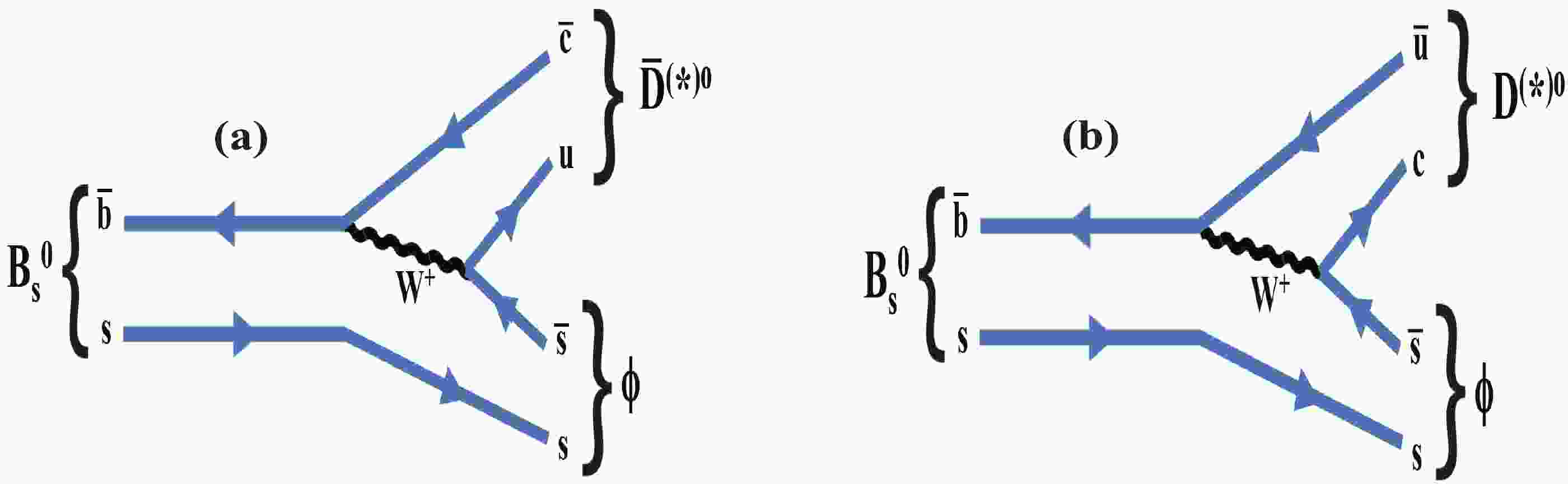
$ {{B^0_s}}\rightarrow {\kern 0.2em\overline{\kern -0.2em D}{}}^{(*)0}\phi $ decays, the observations of which were published by the LHCb experiment in 2013 [21] and 2018 [22], are used to determine$ \gamma $ . A novel method presented in Ref. [22] also demonstrated the feasibility of measuring$ {{B^0_s}}\rightarrow {\kern 0.2em\overline{\kern -0.2em D}{}}^{*0}\phi $ decays with a high purity. A partial reconstruction method is used for the$ {\kern 0.2em\overline{\kern -0.2em D}{}}^{*0} $ meson [23]. A time-integrated method [24-26] was investigated, in which it was shown that information regarding CP violation is preserved in the untagged rate of$ {{B^0_s}}\rightarrow \tilde{D}^{(*)0}\phi $ (or of$ {{B^0}} \rightarrow {{\tilde{D}^0}} {K^0_{\rm{ S}}} $ ), and that if a sufficient number of different D-meson final states is included in the analysis, this decay alone can be used to measure$ \gamma $ in principle. The sensitivity to$ \gamma $ is expected to be much better with the case of the$ {{B^0_s}}\rightarrow \tilde{D}^{(*)0}\phi $ decay than for$ {{B^0}} \rightarrow {{\tilde{D}^0}} {K^0_{\rm{ S}}} $ , as it is proportional to the decay width difference$ y = \Delta\Gamma/{2\Gamma} $ defined in Section II and is equal to$ (6.3\pm0.3) $ % for$ {{B^0_s}} $ mesons and$ (0.05\pm 0.50) $ % for$ {{B^0}} $ [27]. The sensitivity to$ \gamma $ from the$ {{B^0_s}}\rightarrow \tilde{D}^{(*)0}\phi $ modes arises from the interference between two colour-suppressed diagrams, as illustrated in Fig. 1. The relatively large expected value of the ratio of the$ \bar{b}\rightarrow \bar{u}c\bar{s} $ and$ \bar{b}\rightarrow \bar{c}u\bar{s} $ tree-level amplitudes ($20\%-40$ %; see Section IVA) serves as additional motivation for measuring$ \gamma $ in$ {{B^0_s}}\rightarrow \tilde{D}^{(*)0}\phi $ decays. In this study, five neutral D-meson decay modes, namely$ K\pi $ ,$ K3\pi $ ,$ K\pi{{\pi^{0}}} $ ,$ KK $ , and$ \pi\pi $ , are included, the event yields of which are estimated using realistic assumptions based on measurements from LHCb [22, 28, 29]. We justify the choice of these decays and also discuss the case of the two decay modes$ \tilde{D}^0 \rightarrow {K^0_{\rm{ S}}}{{\pi^{+}}}{{\pi^{-}}} $ and$ {K^0_{\rm{ S}}}{{K^{+}}}{{K^{-}}} $ in Section III.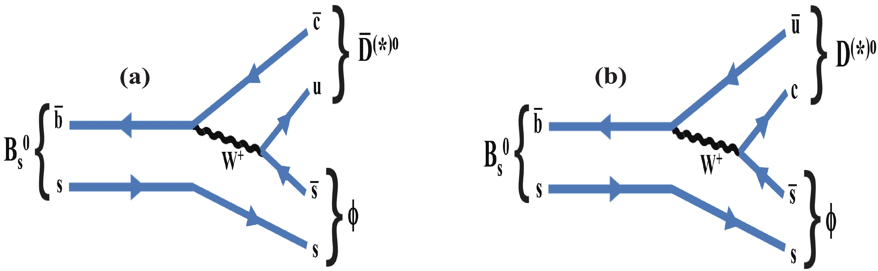
Figure 1. (color online) Feynman diagrams for (a)
${B^0_s}\rightarrow \overline D^{(*)0}\phi$ and (b)${B^0_s}\rightarrow D^{(*)0}\phi$ decays.In Section II, the notations and the selection of the D-meson decay final states are introduced. In Section III, the expected signal yields and their uncertainties are presented. In Section IV, the sensitivity that can be achieved using solely these decays is presented, and further improvements are briefly discussed. In Section V, the future expected precision on
$ \gamma $ with$ {{B^0_s}}\rightarrow {\kern 0.2em\overline{\kern -0.2em D}{}}^{(*)0}\phi $ at LHCb is discussed for the dataset available after LHC Run 3 by 2025 and after a possible second upgrade of LHCb by 2038. Finally, conclusions are presented in Section VI. -
Following the formalism introduced in Refs. [24-26], we define the amplitudes
$ A( {{B^0_s}}\rightarrow {\kern 0.2em\overline{\kern -0.2em D}{}}^{(*)0}\phi) = A^{(*)}_{B}, $

(1) $ A( {{B^0_s}}\rightarrow D^{(*)0}\phi) = A^{(*)}_{B} {{r^{(*)}_{B}}} {\rm e}^{{\rm i}({{\delta^{(*)}_{B}}} +\gamma)}, $

(2) where
$ A^{(*)}_{B} $ and$ r_{B}^{(*)} $ are the magnitude of the$ {{B^0_s}} $ decay amplitude and amplitude magnitude ratio between the suppressed over the favored$ {{B^0_s}} $ decay modes, respectively, whereas$ \delta_{B}^{(*)} $ and$ \gamma $ are the strong and weak phases, respectively. Neglecting mixing and CP violation in the D decays (see, for example, Refs. [30, 31]), the amplitudes into the final state f (denoted below as$ [f]_{D} $ ) and its CP conjugate$ \bar{f} $ are defined as$ A({{\bar{D}^0}} \rightarrow f) = A({{D^0}} \rightarrow \bar{f}) = A_{f}, $

(3) $ A({{D^0}} \rightarrow f) = A({{\bar{D}^0}} \rightarrow \bar{f}) = A_{f} r_{D}^{f} {\rm e}^{{\rm i}\delta_{D}^{f}}, $

(4) where
$ \delta_{D}^{f} $ and$ r_{D}^{f} $ are the strong phase difference and relative magnitude, respectively, between the$ {{D^0}} \rightarrow f $ and$ {{\bar{D}^0}} \rightarrow f $ decay amplitudes.The amplitudes of the full decay chains are given by
$ \begin{aligned}[b] A_{Bf} \equiv & A({{B^0_s}} \rightarrow [f]_{D^{(*)} } \phi )\\ = & A^{(*)}_{B} A^{(*)}_{f} \left[1+{{r^{(*)}_{B}}} r_{D}^{f} {\rm e}^{{\rm i}({{\delta^{(*)}_{B}}} + \delta_{D}^{f} + \gamma)} \right], \end{aligned} $

(5) $ \begin{aligned}[b] A_{B\bar{f}} \equiv & A({{B^0_s}} \rightarrow [\bar{f}]_{D^{(*)} } \phi ) \\ =& A^{(*)}_{B} A^{(*)}_{f} \left[{{r^{(*)}_{B}}} {\rm e}^{{\rm i}({{\delta^{(*)}_{B}}} +\gamma )} + r_{D}^{f} {\rm e}^{{\rm i}\delta_{D}^{f} } \right]. \end{aligned} $

(6) The amplitudes of the CP-conjugate decays are obtained by changing the sign of the weak phase
$ \gamma $ $ \begin{aligned}[b] \bar{A}_{Bf} \equiv & A({{\bar{B}^0_s}} \rightarrow [f]_{D^{(*)}} \phi) \\ =& A^{(*)}_{B} A^{(*)}_{f} \left[{{r^{(*)}_{B}}} {\rm e}^{{\rm i}({{\delta^{(*)}_{B}}} - \gamma)} + r_{D}^{f} {\rm e}^{{\rm i}\delta_{D}^{f} } \right], \end{aligned}$

(7) $\begin{aligned}[b] \bar{A}_{B\bar{f}} \equiv & A({{\bar{B}^0_s}} \rightarrow [\bar{f}]_{D^{(*)}} \phi ) \\ =& A^{(*)}_{B} A^{(*)}_{f} \left[1+{{r^{(*)}_{B}}} r_{D}^{f} {\rm e}^{{\rm i}({{\delta^{(*)}_{B}}} +\delta_{D}^{f} -\gamma)} \right]. \end{aligned} $

(8) Using the standard notations
$ \begin{aligned}[b] & \tau = \Gamma_s t,\quad \Gamma_s = \frac{\Gamma_{L} +\Gamma_{H}}{2},\quad \Delta\Gamma_s = \Gamma_{L}-\Gamma_{H},\\& y = \frac{\Delta \Gamma_s}{2\Gamma_s},\quad \lambda_{f} = \frac{q}{p} . \frac{\bar{A}_{Bf}}{A_{Bf}}, \end{aligned} $

and assuming that
$ |q/p| = 1 $ ($ |q/p| = 1.0003\pm 0.0014 $ [32]), the untagged decay rate for the decay$ {{B^0_s}}/{{\bar{B}^0_s}} \rightarrow [f]_{D^{(*)}} \phi $ is obtained by Eq. (10) of Ref. [33]:$ \begin{aligned}[b] \frac{{\rm d}\Gamma ({{B^0_s}}(\tau) \rightarrow [f]_{D^{(*)}} \phi )}{{\rm d}\tau } + \frac{{\rm d}\Gamma({{\bar{B}^0_s}}(\tau) \rightarrow [f]_{D^{(*)}} \phi )}{{\rm d}\tau } \propto e^{-\tau } |A_{Bf}|^{2} \times \left[(1+\left|\lambda_{f} \right|^{2})\cosh(y\tau)-2{\rm{Re}}(\lambda_{f})\sinh(y\tau)\right]. \end{aligned} $

(9) -
Experimentally, owing to the trigger and selection requirements as well as inefficiencies in the reconstruction, the decay time distribution is affected by the acceptance effects. The acceptance correction has been estimated from pseudoexperiments based on a related publication by the LHCb collaboration [34]. It is described by an empirical acceptance function
$ \varepsilon_{ta}(\tau ) = \frac{(\alpha \tau )^{\beta }}{1+(\alpha \tau )^{\beta }}(1-\xi \tau ), $

(10) with
$ \alpha = 1.5 $ ,$ \beta = 2.5 $ , and$ \xi = 0.01 $ .Taking into account this effect, the time-integrated untagged decay rate is
$ \begin{aligned}[b] \Gamma({{\tilde{B}^0_s}} \rightarrow [f]_{D^{(*)} } \phi ) =& \int_{0}^{\infty}\left[\frac{{\rm d}\Gamma ({{B^0_s}}(\tau) \rightarrow [f]_{D^{(*)}} \phi)}{{\rm d}\tau} \right.\\& \left.+ \frac{{\rm d}\Gamma({{\bar{B}^0_s}}(\tau )\rightarrow [f]_{D^{(*)}} \phi)}{{\rm d}\tau } \right] \varepsilon_{ta}(\tau ) {\rm d}\tau. \end{aligned} $

(11) By defining the function
$ g(x) = \int_{0}^{\infty}\frac{e^{-x\tau} (1+\xi \tau (\alpha \tau)^{\beta})}{1+(\alpha \tau )^{\beta }}{\rm d}\tau, $

(12) and using Eq. (9), one obtains
$ \Gamma({{B^0_s}} \rightarrow [f]_{D} \phi)\propto \left|A_{Bf} \right|^{2} \left[(1+\left|\lambda_{f} \right|^{2} ){\cal{A}}-2y{\rm{Re}}(\lambda_{f}){\cal{B}}\right], $

(13) where
$ {\cal{A}} = 1-[g(1-y)+g(1+y)]/2 $ and$ {\cal{B}} = 1-[g(1-y)- $ $g(1+y)]/2y $ . With$ y = (0.128\pm 0.009)/2 $ for the$ {{B^0_s}} $ meson [27], one obtains$ {\cal{A}} = 0.488\pm 0.005 $ and$ {\cal{B}} = 0.773\pm 0.008 $ . Examples of decay-time acceptance distributions are displayed in Fig. 2.
Figure 2. (color online) Examples of decay-time acceptance distributions for three different sets of parameters
$\alpha$ ,$\beta$ , and$\xi$ (nominal in green). -
The D-meson decays are reconstructed in quasi flavor-specific modes
$ f^{-}(\equiv f) = {{K^{-}}} {{\pi^{+}}} $ ,$ {{K^{-}}} 3\pi $ , and$ {{K^{-}}} {{\pi^{+}}} \pi^{0} $ ; their CP-conjugate modes$ f^{+}(\equiv \bar{f}) = {{K^{+}}} {{\pi^{-}}} $ ,$ {{K^{+}}} 3\pi $ , and$ {{K^{+}}} {{\pi^{-}}} \pi^{0} $ ; and CP-eigenstate modes$ f_{CP} = {{K^{+}}} {{K^{-}}} $ and$ {{\pi^{+}}} {{\pi^{-}}} $ .In the following, we introduce the weak phase
$ \beta_{s} $ that is defined as$ \beta_{s} = \arg \left(-\dfrac{V_{ts} V_{tb}^{*} }{V_{cs} V_{cb}^{*} } \right) $ . From Eqs. (5), (7), and (13) and with$\lambda_{f} = {\rm e}^{2{\rm i}\beta_{s}}\dfrac{\bar{A}_{Bf}}{A_{Bf}}$ , for a given number of untagged$ {{B^0_s}} $ mesons produced in the$ pp $ collisions at the LHCb interaction point,$ N({{B^0_s}}) $ , we can compute the number of$ {{B^0_s}}\rightarrow {{\bar{D}^0}} \phi $ decays with the D meson decaying into the final state$ f^{-} $ . For the reference decay mode$ f^{-} \equiv {{K^{-}}} {{\pi^{+}}} $ , we obtain$ \begin{aligned} N\left({{B^0_s}} \rightarrow \left[{{K^{-}}} {{\pi^{+}}} \right]_{D} \left[{{K^{+}}} {{K^{-}}} \right]_{\phi } \right) = C_{K\pi}\Big[-2{\cal{B}} y {{r_{B}}} \cos \left({{\delta_{B}}} + 2\beta_{s} - \gamma \right) + {\cal{A}} \left(1+{{r_{B}}}^{2} +4 {{r_{B}}} r_{D}^{K\pi} \cos {{\delta_{B}}} \cos \left(\delta_{D}^{K\pi } + \gamma \right)\right)\Big], \end{aligned}$

(14) in which the terms proportional to
$ (r_{D}^{K\pi})^{2} \ll 1 $ and$ y r_{D}^{K\pi } \ll 1 $ have been neglected ($ r_{D}^{K\pi} = 5.90^{+0.34}_{-0.25}$ % [27]). The best approximation for the scale factor$ C_{K\pi} $ is$ \begin{aligned}[b] C_{K\pi } =& N({{B^0_s}})\times \varepsilon({{B^0_s}} \rightarrow \left[{{K^{-}}} {{\pi^{+}}} \right]_{D} \left[{{K^{+}}} {{K^{-}}} \right]_{\phi})\\ &\times Br({{B^0_s}} \rightarrow \left[{{K^{-}}} {{\pi^{+}}} \right]_{D} \left[{{K^{+}}} {{K^{-}}} \right]_{\phi}), \end{aligned} $

(15) where
$ \varepsilon({{B^0_s}} \rightarrow \left[{{K^{-}}} {{\pi^{+}}} \right]_{D} \left[{{K^{+}}} {{K^{-}}} \right]_{\phi}) $ is the global detection efficiency of this decay mode, and$ Br({{B^0_s}} \rightarrow \left[{{K^{-}}} {{\pi^{+}}} \right]_{D}$ $ \left[{{K^{+}}} {{K^{-}}} \right]_{\phi}) $ is its branching fraction. The value of the scale factor$ C_{K\pi} $ is estimated from the LHCb Run 1 data [22], the average$ f_{s}/f_{d} $ of the b-hadron production fraction ratio measured by LHCb [35], and the different branching fractions [32].For better numerical behavior, we use the Cartesian coordinate parameterization
$ x_{\pm}^{(*)} = {{r^{(*)}_{B}}} \cos ({{\delta^{(*)}_{B}}} \pm \gamma ) \ \ {\rm{and}} \quad y_{\pm}^{(*)} = {{r^{(*)}_{B}}} \sin({{\delta^{(*)}_{B}}} \pm \gamma). $

(16) Subsequently, Eq. (14) becomes
$ \begin{aligned}[b] N\left({{B^0_s}} \rightarrow \left[{{K^{-}}} {{\pi^{+}}} \right]_{D} \left[{{K^{+}}} {{K^{-}}} \right]_{\phi } \right) =& C_{K\pi} \Big[ -2 {\cal{B}} y \left[x_{-} \cos(2\beta_{s}) - y_{-} \sin(2\beta_{s}) \right] \\&+ {\cal{A}} \Big( 1+x_{-}^{2} +y_{-}^{2} + 2r_{D}^{K\pi} [(x_{+} +x_{-}) \cos \delta_{D}^{K\pi} - (y_{+} -y_{-}) \sin \delta_{D}^{K\pi} ] \Big)\Big]. \end{aligned} $

(17) For three and four body final states
$ K3\pi $ and$ K\pi \pi^{0} $ , multiple interfering amplitudes exist; therefore, their amplitudes and phases$ \delta_{D}^{f} $ vary across the decay phase space. However, an analysis that is integrated over the phase space can be performed in a very similar manner to two body decays with the inclusion of an additional parameter, namely the so-called coherence factor$ R_{D}^{f} $ , which has been measured in previous experiments [36]. The strong phase difference$ \delta_{D}^{f} $ is then treated as an effective phase that is averaged over all amplitudes. For these modes, we obtain an expression similar to (17):$ \begin{aligned}[b] N\left({{B^0_s}} \rightarrow \left[f^{-} \right]_{D} \left[{{K^{+}}} {{K^{-}}} \right]_{\phi} \right) = &C_{K\pi} F_{f} \Big[ -2 {\cal{B}} y\left[x_{-} \cos \left(2\beta_{s} \right) - y_{-} \sin \left(2\beta_{s} \right)\right] \\&+ {\cal{A}} \Big(1+x_{-}^{2} + y_{-}^{2} + 2r_{D}^{f} R_{D}^{f} \left[\left(x_{+} +x_{-} \right)\cos \delta_{D}^{f} -\left(y_{+} -y_{-} \right)\sin \delta_{D}^{f} \right]\Big)\Big], \end{aligned} $

(18) where
$ F_{f} $ is the scale factor of the f decay relative to the$ K\pi $ decay and depends on the ratios of detection efficiencies and branching fractions of the corresponding modes$ \begin{aligned}[b] F_{f} =& \frac{C_{f}}{C_{K\pi}} = \frac{\varepsilon(D\rightarrow f)}{\varepsilon (D\rightarrow K\pi )} \\&\times \frac{[Br({{D^0}} \rightarrow f) + Br({{\bar{D}^0}} \rightarrow f)]}{[Br({{D^0}} \rightarrow {{K^{-}}} {{\pi^{+}}})+Br({{\bar{D}^0}} \rightarrow {{K^{-}}} {{\pi^{+}}})]}. \end{aligned} $

(19) The value of
$ F_{f} $ for the different modes used in this study is determined from the LHCb measurements in the$ B^{\pm} \rightarrow DK^{\pm} $ and$ B^{\pm} \rightarrow D\pi^{\pm } $ modes, with two or four-body D decays [28, 29].The time-integrated untagged decay rate for
$ {{B^0_s}} \rightarrow [\bar{f}]_{D} \phi $ is given by Eq. (13) by substituting$ A_{Bf} \rightarrow \bar{A}_{B\bar{f}} $ and$\lambda_{f} \rightarrow \bar{\lambda}_{\bar{f}} = \lambda_{f}^{-1} = {\rm e}^{-2{\rm i}\beta_{s}} (A_{B\bar{f}}/\bar{A}_{B\bar{f}})$ , which is equivalent to the change$ \beta_{s} \rightarrow -\beta_{s} $ and$ \gamma \rightarrow -\gamma $ (i.e.,$ x_{\pm} \rightarrow x_{\mp} $ and$ y_{\pm} \rightarrow y_{\mp} $ ). Therefore, the observables are$ \begin{aligned}[b] N\left({{B^0_s}} \rightarrow \left[{{K^{+}}} {{\pi^{-}}} \right]_{D} \left[{{K^{+}}} {{K^{-}}} \right]_{\phi} \right) =& C_{K\pi} \Big[ -2 {\cal{B}} y\left[x_{+} \cos \left(2\beta_{s} \right)+y_{+} \sin \left(2\beta_{s} \right)\right] \\&+ {\cal{A}} \Big(1+x_{+}^{2} +y_{+}^{2} + 2r_{D}^{K\pi} \left[\left(x_{+} +x_{-} \right)\cos \delta_{D}^{K\pi} + \left(y_{+} -y_{-} \right)\sin \delta_{D}^{K\pi} \right]\Big)\Big], \end{aligned} $

(20) and for the modes
$ f^{+} \equiv {{K^{+}}} 3\pi $ ,$ {{K^{+}}} {{\pi^{-}}} \pi^{0} $ $ \begin{aligned}[b] N\left({{B^0_s}} \rightarrow \left[f^{+} \right]_{D} \left[{{K^{+}}} {{K^{-}}} \right]_{\phi } \right) =& C_{K\pi} F_{f} \Big[ -2{\cal{B}} y\left[x_{+} \cos \left(2\beta_{s} \right)+y_{+} \sin \left(2\beta_{s} \right)\right] \\ &+ {\cal{A}} \Big(1+x_{+}^{2} +y_{+}^{2} + 2r_{D}^{f} R_{f} \left[\left(x_{+} +x_{-} \right)\cos \delta_{D}^{f} +\left(y_{+} -y_{-} \right)\sin \delta_{D}^{f} \right]\Big)\Big]. \end{aligned} $

(21) Obviously, any significant asymmetries on the yield of the observable corresponding to Eq. (17) with respect to Eq. (20), or Eq. (18) with respect to Eq. (21), are a clear signature for CP violation.
For the CP-eigenstate modes
$ D\rightarrow h^{+} h^{-} \, (h\equiv K,\, \pi ) $ , we have$ r_{D} = 1 $ and$ \delta_{D} = 0 $ . By following the same approach as that for quasi flavor-specific modes, the observables can be written as$ \begin{aligned}[b] N\left({{B^0_s}} \rightarrow \left[h^{+} h^{-} \right]_{D} \left[{{K^{+}}} {{K^{-}}} \right]_{\phi} \right) =&4 C_{K\pi } F_{hh} \Big[ {\cal{A}} \left(1+x_{+}^{2} +y_{+}^{2} +x_{+} +x_{-} \right) - {\cal{B}} y \Big( \left(1+x_{+} +x_{-} +x_{+} x_{-} +y_{+} y_{-} \right)\cos \left(2\beta_{s} \right)\\ &+ \left(y_{+} -y_{-} +y_{+} x_{-} -x_{+} y_{-} \right)\sin \left(2\beta_{s} \right) \Big) \Big]. \end{aligned}$

(22) Analogous to
$ F_{f} $ ,$ F_{hh} $ is defined as$ \begin{aligned} F_{hh} = \frac{C_{hh} }{C_{K\pi} } = \frac{\varepsilon (D\rightarrow hh)}{\varepsilon(D\rightarrow K\pi )} \times \frac{Br({{D^0}} \rightarrow hh)}{[Br({{D^0}} \rightarrow {{K^{-}}} {{\pi^{+}}})+ Br({{\bar{D}^0}} \rightarrow {{K^{-}}} {{\pi^{+}}} )]} \end{aligned} $

(23) and their values are determined in the same manner as
$ F_{f} $ .For the modes
$ {K^0_{\rm{ S}}}{{\pi^{+}}}{{\pi^{-}}} $ and$ {K^0_{\rm{ S}}}{{K^{+}}}{{K^{-}}} $ (i.e.,$ {K^0_{\rm{ S}}} hh $ ), we obtain$ \begin{aligned}[b] N\left({{B^0_s}} \rightarrow \left[ {K^0_{\rm{ S}}} hh\right]_{D} \left[{{K^{+}}} {{K^{-}}} \right]_{\phi } \right) =& 2 C_{K\pi} F_{{K^0_{\rm{ S}}} hh} \times \Big[ -{\cal{B}} y \left[(x_{+}+x_{-}) \cos(2\beta_{s}) +(y_{+}-y_{-}) \sin(2\beta_{s})\right] + {\cal{A}} \Big( 1 +x_{-}^{2} +y_{-}^{2} + 2 (x_{+} +x_{-}) \\ &\times r_{D}^{{K^0_{\rm{ S}}} hh}(m^2_+,m^2_-) \kappa_{D}^{{K^0_{\rm{ S}}} hh}(m^2_{+},m^2_{-}) \cos \delta_{D}^{{K^0_{\rm{ S}}} hh}(m^2_{+},m^2_{-}) \Big) \Big], \end{aligned}$

(24) where
$ F_{{K^0_{\rm{ S}}} hh} $ is defined as in Eq. (23). The strong parameters$ r_{D}^{{K^0_{\rm{ S}}} hh}(m^2_+,m^2_-) $ ,$ \kappa_{D}^{{K^0_{\rm{ S}}} hh}(m^2_+,m^2_-) $ , and$ \cos \delta_{D}^{{K^0_{\rm{ S}}} hh}(m^2_+,m^2_-) $ vary over the Dalitz plot$ (m^2_+,m^2_-)\equiv (m^2({K^0_{\rm{ S}}}{{\pi^{+}}}), \ m^2({K^0_{\rm{ S}}}{{\pi^{-}}})) $ and are defined in Section III. -
For the
$ {{D^{*0}}}$ decays, we consider the two modes$ {{D^{*0}}}\rightarrow {{D^0}} \pi^{0} $ and$ {{D^{*0}}} \rightarrow {{D^0}} \gamma $ , where the$ {{D^0}} $ mesons are reconstructed, as in the above, in quasi flavor-specific modes$ K\pi $ ,$ K3\pi $ , and$ K\pi \pi^{0} $ as well as CP-eigenstate modes$ \pi \pi $ and$ KK $ . As demonstrated in Ref. [37], the formalism for the cascade$ {{B^0_s}} \rightarrow {{\bar{D}^{*0}}} \phi ,\; {{\bar{D}^{*0}}} \rightarrow {{\bar{D}^0}} \pi^{0} $ is similar to that of$ {{B^0_s}} \rightarrow {{\bar{D}^0}} \phi $ . Therefore, the relevant observables can be written similarly to Eqs. (17), (18), (20), (21), and (22), by substituting$ C_{K\pi} \rightarrow C_{K\pi,D {{\pi^{0}}}} $ ,$ {{r_{B}}} \rightarrow {{r^*_{B}}} $ , and$ {{\delta_{B}}} \rightarrow {{\delta^*_{B}}} $ ($ x_{\pm} \rightarrow x_{\pm}^{*} $ and$ y_{\pm} \rightarrow y_{\pm}^{*} $ ):$ \begin{aligned}[b] N\left({{B^0_s}} \rightarrow \left[\left[{{K^{-}}} {{\pi^{+}}} \right]_{D} \pi^{0} \right]_{D^{*}} \left[{{K^{+}}} {{K^{-}}} \right]_{\phi} \right) =&C_{K\pi,D{{\pi^{0}}}} \Big[ -2 {\cal{B}} y\left[x_{-}^{*} \cos \left(2\beta_{s} \right)-y_{-}^{*} \sin \left(2\beta_{s} \right)\right] \\ & +{\cal{A}} \Big(1+x_{-}^{*2} +y_{-}^{*2}+ 2r_{D}^{K\pi} \left[\left(x_{+}^{*} +x_{-}^{*} \right)\cos \delta_{D}^{K\pi} - \left(y_{+}^{*} - y_{-}^{*} \right) \sin \delta_{D}^{K\pi} \right]\Big)\Big], \end{aligned}$

(25) $ \begin{aligned}[b] N\left({{B^0_s}} \rightarrow \left[\left[{{K^{+}}} {{\pi^{-}}} \right]_{D} \pi^{0} \right]_{D^{*}} \left[{{K^{+}}} {{K^{-}}} \right]_{\phi } \right) =&C_{K\pi,D{{\pi^{0}}}} \Big[ -2 {\cal{B}} y\left[x_{+}^{*} \cos \left(2\beta_{s} \right)+y_{+}^{*} \sin \left(2\beta_{s} \right)\right] \\ &+{\cal{A}} \Big(1+x_{+}^{*2} + y_{+}^{*2} + 2r_{D}^{K\pi} \left[ \left(x_{+}^{*} + x_{-}^{*} \right)\cos \delta_{D}^{K\pi} + \left(y_{+}^{*} - y_{-}^{*} \right) \sin \delta_{D}^{K\pi} \right]\Big)\Big], \end{aligned} $

(26) $ \begin{aligned}[b] \;\;N\left({{B^0_s}} \rightarrow \left[\left[f^{-} \right]_{D} \pi^{0} \right]_{D^{*} } \left[{{K^{+}}} {{K^{-}}} \right]_{\phi} \right) =& C_{K\pi,D{{\pi^{0}}}} F_{f} \Big[ - 2 {\cal{B}} y\left[x_{-}^{*} \cos \left(2\beta_{s} \right)-y_{-}^{*} \sin \left(2\beta_{s} \right)\right] \\ &+{\cal{A}} \Big(1+x_{-}^{*2} +y_{-}^{*2} + 2r_{D}^{f} R_{f} \left[\left(x_{+}^{*} +x_{-}^{*} \right)\cos \delta_{D}^{f} -\left(y_{+}^{*} -y_{-}^{*} \right)\sin \delta_{D}^{f} \right]\Big)\Big], \end{aligned}$

(27) $ \begin{aligned}[b] \;\;N\left({{B^0_s}} \rightarrow \left[\left[f^{+} \right]_{D} \pi^{0} \right]_{D^{*}} \left[{{K^{+}}} {{K^{-}}} \right]_{\phi} \right) = &C_{K\pi,D{{\pi^{0}}}} F_{f} \Big[ -2{\cal{B}} y\left[x_{+}^{*} \cos \left(2\beta_{s} \right)+y_{+}^{*} \sin \left(2\beta_{s} \right)\right] \\ &+ {\cal{A}} \Big(1+x_{+}^{*2} +y_{+}^{*2} + 2r_{D}^{f} R_{f} \left[\left(x_{+}^{*} +x_{-}^{*} \right)\cos \delta_{D}^{f} +\left(y_{+}^{*} -y_{-}^{*} \right)\sin \delta_{D}^{f} \right]\Big)\Big], \end{aligned}$

(28) $ \begin{aligned}[b] N\left({{B^0_s}} \rightarrow \left[\left[h^{+} h^{-} \right]_{D} \pi^{0} \right]_{D^{*}} \left[{{K^{+}}} {{K^{-}}} \right]_{\phi} \right) =& 4 C_{K\pi,D{{\pi^{0}}}} F_{hh} \Big[ {\cal{A}} \left(1+x_{+}^{*2} +y_{+}^{*2} +x_{+}^{*} +x_{-}^{*} \right) - {\cal{B}} y \Big( \left(1+x_{+}^{*} +x_{-}^{*} +x_{+}^{*} x_{-}^{*} +y_{+}^{*} y_{-}^{*} \right)\cos \left( 2\beta_{s} \right)\\ &+\left(y_{+}^{*} -y_{-}^{*} +y_{+}^{*} x_{-}^{*} -x_{+}^{*} y_{-}^{*} \right)\sin \left(2\beta_{s} \right) \Big)\Big]. \end{aligned} $

(29) In the case of
$ {{D^{*0}}} \rightarrow {{D^0}} \gamma $ , the formalism is very similar, except that there is an effective strong phase shift of$ \pi $ with respect to$ {{D^{*0}}} \rightarrow {{D^0}} \pi^{0} $ [37]. The observables can be derived from the previous ones by substituting$ C_{K\pi,D{{\pi^{0}}}} \rightarrow C_{K\pi,D\gamma} $ and$ \delta_{B}^{*} \rightarrow \delta_{B}^{*} +\pi $ (i.e.$ x_{\pm}^{*} \rightarrow -x_{\pm}^{*} $ and$ y_{\pm}^{*} \rightarrow -y_{\pm}^{*} $ ):$ \begin{aligned}[b] \;\;N\left({{B^0_s}} \rightarrow \left[\left[{{K^{-}}} {{\pi^{+}}} \right]_{D} \gamma \right]_{D^{*}} \left[{{K^{+}}} {{K^{-}}} \right]_{\phi} \right) =&C_{K\pi,D\gamma } \Big[ 2 {\cal{B}} y\left[x_{-}^{*} \cos \left(2\beta_{s} \right)-y_{-}^{*} \sin \left(2\beta_{s} \right)\right] \\& + {\cal{A}} \Big(1+x_{-}^{*2} +y_{-}^{*2} +2r_{D}^{K\pi} \left[-\left(x_{+}^{*} +x_{-}^{*} \right)\cos \delta_{D}^{K\pi} +\left(y_{+}^{*} -y_{-}^{*} \Big)\sin \delta_{D}^{K\pi } \right]\right)\Big], \end{aligned}$

(30) $ \begin{aligned}[b] \;\;N\left({{B^0_s}} \rightarrow \left[\left[{{K^{+}}} {{\pi^{-}}} \right]_{D} \gamma \right]_{D^{*}} \left[{{K^{+}}} {{K^{-}}} \right]_{\phi} \right) =&C_{K\pi,D\gamma} \Big[2 {\cal{B}} y\left[x_{+}^{*} \cos \left(2\beta_{s} \right)+y_{+}^{*} \sin \left(2\beta_{s} \right)\right] \\&+{\cal{A}} \Big(1+x_{+}^{*2} +y_{+}^{*2} + 2r_{D}^{K\pi} \left[-\left(x_{+}^{*} +x_{-}^{*} \right)\cos \delta_{D}^{K\pi } -\left(y_{+}^{*} -y_{-}^{*} \Big)\sin \delta_{D}^{K\pi } \right]\right)\Big], \end{aligned}$

(31) $ \begin{aligned}[b] N\left({{B^0_s}} \rightarrow \left[\left[f^{-} \right]_{D} \gamma \right]_{D^{*}} \left[{{K^{+}}} {{K^{-}}} \right]_{\phi} \right) = &C_{K\pi,D\gamma} F_{f} \Big[2 {\cal{B}} y\left[x_{-}^{*} \cos \left(2\beta_{s} \right)-y_{-}^{*} \sin \left(2\beta_{s} \right)\right] \\&+ {\cal{A}} \Big(1+x_{-}^{*2} +y_{-}^{*2} + 2r_{D}^{f} R_{f} \left[-\left(x_{+}^{*} +x_{-}^{*} \right)\cos \delta_{D}^{f} +\left(y_{+}^{*} -y_{-}^{*} \Big)\sin \delta_{D}^{f} \right]\right)\Big], \end{aligned}$

(32) $ \begin{aligned}[b] N\left({{B^0_s}} \rightarrow \left[\left[f^{+} \right]_{D} \gamma \right]_{D^{*}} \left[{{K^{+}}} {{K^{-}}} \right]_{\phi} \right) =&C_{K\pi,D\gamma} F_{f} \Big[2 {\cal{B}} y\left[x_{+}^{*} \cos \left(2\beta_{s} \right)+y_{+}^{*} \sin \left(2\beta_{s} \right)\right]\\& + {\cal{A}} \Big(1+x_{+}^{*2} +y_{+}^{*2} + 2r_{D}^{f} R_{f} \left[-\left(x_{+}^{*} +x_{-}^{*} \right) \cos \delta_{D}^{f} - \left(y_{+}^{*} -y_{-}^{*} \right)\sin \delta_{D}^{f} \right]\Big)\Big], \end{aligned}$

(33) $ \begin{aligned}[b] N\left({{B^0_s}} \rightarrow \left[\left[h^{+} h^{-} \right]_{D} \gamma \right]_{D^{*} } \left[{{K^{+}}} {{K^{-}}} \right]_{\phi} \right) = & 4C_{K\pi,D\gamma} F_{hh} \Big[ {\cal{A}} \left(1+x_{+}^{*2} +y_{+}^{*2} -x_{+}^{*} -x_{-}^{*} \right) - {\cal{B}} y \Big( \left(1-x_{+}^{*} -x_{-}^{*} +x_{+}^{*} x_{-}^{*} +y_{+}^{*} y_{-}^{*} \right) \cos \left(2\beta_{s} \right) \\ & + \left(-y_{+}^{*} + y_{-}^{*} + y_{+}^{*} x_{-}^{*} -x_{+}^{*} y_{-}^{*} \right)\sin \left(2\beta_{s} \right) \Big) \Big]. \end{aligned} $

(34) $ C_{K\pi,D\pi^{0}} $ and$ C_{K\pi,D\gamma} $ are determined in the same manner as$ C_{K\pi } $ , i.e., from the LHCb Run 1 data [22] and taking into account the fraction of longitudinal polarization in the decay$ {{B^0_s}} \rightarrow {{D^{*0}}} \phi $ ,$ f_{L} = (73\pm 15\pm 4) $ % [22], and the branching fractions$ Br({{\bar{D}^{*0}}} \rightarrow {{\bar{D}^0}} \pi^{0}) $ and$ Br({{\bar{D}^{*0}}} \rightarrow {{\bar{D}^0}} \gamma) $ [32]. -
The LHCb collaboration has measured the yields of the
$ {{B^0_s}}\rightarrow \tilde{D}^{(*)0}\phi $ and$ \tilde{D}^0\rightarrow K\pi $ modes using Run 1 data, corresponding to an integrated luminosity of 3$ {{\rm{fb}}^{-1}} $ (Ref. [22]). Taking into account the cross-section differences among different center-of-mass energies, the equivalent integrated luminosities in different data over several years from LHCb are summarized in Table 1. The corresponding expected yields of the$ \tilde{D}^0 $ meson decaying into other modes are also estimated according to Refs. [28], [29], and [41]. The scaled results are listed in Table 2, where the longitudinal polarization fraction$ f_L \!=\! (73\!\pm \!15\!\pm\! 4)\; $ % [22] of$ {{B^0_s}}\!\rightarrow\! \tilde{D}^{*0}\phi $ is considered so that the CP eigenvalue of the final state is well defined and is similar to that of the$ {{B^0_s}}\rightarrow \tilde{D}^{0}\phi $ mode.Years/Run $ \sqrt{s} $ /TeV

Int. lum./fb−1 Cross section Equiv. 7 TeV data 2011 7 1.1 $\sigma_{2011}=38.9\; {\rm{\mu b} }$ 

1.1 2012 8 2.1 $ 1.17 \times \sigma_{2011} $ 

2.4 Run 1 − 3.2 − 3.5 2015 to 2018 (Run 2) 13 5.9 $ 2.00 \times \sigma_{2011} $ 

11.8 Total − 9.1 − 15.3 Expect. yield (Run 1 only) $ {{B^0_s}}\rightarrow \tilde{D}^0(K\pi)\phi $ 

$ 577 $ (

$ 132\pm 13 $ [22])

$ {{B^0_s}}\rightarrow \tilde{D}^0(K3\pi)\phi $ 

$ 218 $ 

$ {{B^0_s}}\rightarrow \tilde{D}^0(K\pi{{\pi^{0}}})\phi $ 

$ 58 $ 

$ {{B^0_s}}\rightarrow \tilde{D}^0(KK)\phi $ 

$ 82 $ 

$ {{B^0_s}}\rightarrow \tilde{D}^0(\pi\pi)\phi $ 

$ 24 $ 

$ {{B^0_s}}\rightarrow \tilde{D}^0({K^0_{\rm{ S}}} \pi\pi)\phi $ 

$ 54 $ 

$ {{B^0_s}}\rightarrow \tilde{D}^0({K^0_{\rm{ S}}} KK)\phi $ 

$ 8 $ 

$ {{B^0_s}}\rightarrow \tilde{D}^{*0}\phi $ mode

$ D^0{{\pi^{0}}} $ 

$ D^0\gamma $ 

$ {{B^0_s}}\rightarrow \tilde{D}^{*0}(K\pi)\phi $ 

$ 337 $ 

$ 184 $ 

(119 [22]) $ {{B^0_s}}\rightarrow \tilde{D}^{*0}(K3\pi)\phi $ 

$ 127 $ 

$ 69 $ 

$ {{B^0_s}}\rightarrow \tilde{D}^{*0}(K\pi{{\pi^{0}}})\phi $ 

$ 34 $ 

$ 18 $ 

$ {{B^0_s}}\rightarrow \tilde{D}^{*0}(KK)\phi $ 

$ 48 $ 

$ 26 $ 

$ {{B^0_s}}\rightarrow \tilde{D}^{*0}(\pi\pi)\phi $ 

$ 14 $ 

$ 8 $ 

Table 2. Expected yield of each mode for
$ 9.1 {{\rm{fb}}^{-1}} $ (Run 1 and Run 2 data). The expected yields for the$ {{B^0_s}}\rightarrow \tilde{D}^{*0}\phi $ sub-modes are scaled by the longitudinal fraction of polarization$ f_L = (73\pm15) $ %. To be scaled by 6.3 (90) for prospects after 2025 (2038) (see Section V).Several additional parameters are used in the sensitivity study, as indicated in Table 3. Most of these originate from D decays, and the scale factors F are calculated by using the data from Refs. [28] and [29], as well as the branching fractions from PDG [32].
Parameter Value −2 $ \beta_S $ [mrad]

$ -36.86\pm0.82 $ [42]

$ y=\Delta\Gamma_s/2\Gamma_s $ (%)

$ 6.40\pm0.45 $ [27]

$ r^{K\pi}_D $ (%)

$ 5.90^{+0.34}_{-0.25} $ [27]

$ \delta^{K\pi}_D $ [deg]

$ 188.9^{+8.2}_{-8.9} $ [27]

$ r^{K3\pi}_D $ (%)

$ 5.49\pm0.06 $ [36]

$ R^{K3\pi}_D $ (%)

$ 43^{+17}_{-13} $ [36]

$ \delta^{K3\pi}_D $ [deg]

$ 128^{+28}_{-17} $ [36]

$ r^{K\pi{{\pi^{0}}}}_D $ (%)

$ 4.47\pm0.12 $ [36]

$ R^{K\pi{{\pi^{0}}}}_D $ (%)

$ 81\pm6 $ [36]

$ \delta^{K\pi{{\pi^{0}}}}_D $ [deg]

$ 198^{+14}_{-15} $ [36]

Scale factor (w.r.t. $ K\pi $ )

(Stat. uncertainty only) $ F_{K3\pi} $ (%)

$ 37.8\pm0.1 $ [28]

$ F_{K\pi{{\pi^{0}}}} $ (%)

$ 10.0\pm0.1 $ [29]

$ F_{KK} $ (%)

$ 14.2\pm 0.1 $ [28]

$ F_{\pi\pi} $ (%)

$ 4.2\pm0.1 $ [28]

Table 3. Other external parameters used in sensitivity study. The scale factors F are also listed.
The expected numbers of signal events are also calculated from the full expressions provided in Sections IIB and IIC by using the detailed branching fraction derivations explained in Ref. [22], as well as scaling by the LHCb Run 1 and Run 2 integrated luminosities, as listed in Table 1. The obtained normalization factors
$ C_{K\pi} $ ,$ C_{K\pi,D{{\pi^{0}}}} $ , and$ C_{K\pi,D\gamma} $ are$ 608\pm67 $ ,$ 347\pm56 $ , and$ 189\pm31 $ , respectively. To compute the uncertainty on the normalization factors, we assume that it is possible to improve the global uncertainty on the measurement of the branching fraction of the decay modes$ {{B^0_s}}\rightarrow {\kern 0.2em\overline{\kern -0.2em D}{}}^{(*)0}\phi $ , and of the polarization of the mode$ {{B^0_s}}\rightarrow {\kern 0.2em\overline{\kern -0.2em D}{}}^{*0}\phi $ , by a factor of 2 when adding the LHCb data from Run 2 [22]. The values of the three normalization factors are in good agreement with the yields listed in Table 2.The number of expected event yields and the value of the coherence factor
$ R_D $ listed in Tables 2 and 3 justify a posteriori our choice of performing the sensitivity study on$ \gamma $ with the D-meson decay modes$ K\pi $ ,$ K3\pi $ ,$ K\pi{{\pi^{0}}} $ ,$ KK $ and$ \pi\pi $ . By definition, the value of$ R_D $ is 1 for two-body decays and$ r_D = 1 $ for CP-eigenstates, whereas for$ K3\pi $ ,$ R_D $ is approximately$ 43 $ % and larger, namely$ 81 $ %, for$ K\pi{{\pi^{0}}} $ . A larger$ R_D $ results in stronger sensitivity to$ \gamma $ . According to Eqs. (20), (21), and (22), it is clear that the largest sensitivity to$ \gamma $ is expected to originate from the ordered$ {{D^0}} $ decay modes:$ KK $ ,$ \pi\pi $ ,$ K\pi $ ,$ K\pi{{\pi^{0}}} $ , and$ K3\pi $ , for the same number of selected events. Therefore, even with lower yields, the modes$ K\pi{{\pi^{0}}} $ and$ \pi\pi $ should be of interest; this is discussed in Section IV I.Returning to the modes
$ {{D^0}}\rightarrow {K^0_{\rm{ S}}}\pi\pi $ and$ {K^0_{\rm{ S}}} KK $ , the scale factors are$ F_{{K^0_{\rm{ S}}}\pi\pi} = (9.3\pm0.1) $ % and$ F_{{K^0_{\rm{ S}}} KK} =$ $ (1.4\pm0.1) $ % [41]. The strong parameters$ r_{D}^{{K^0_{\rm{ S}}} hh}(m^2_+,m^2_-) $ ,$ \kappa_{D}^{{K^0_{\rm{ S}}} hh}(m^2_+,m^2_-) $ , and$ \cos \delta_{D}^{{K^0_{\rm{ S}}} hh}(m^2_+,m^2_-) $ can be defined according the effective method presented in Ref. [43], by using quantum-correlated$ {{\tilde{D}^0}} $ decays, in which the phase space$ (m^2_+, \ m^2_-) $ is divided into$ {\cal{N}} $ tailored regions or “bins” [44], such that in the bin of index i,$\begin{aligned}[b] \sqrt{K_i/K_{-i}} =& r_{D,i}^{{K^0_{\rm{ S}}} hh},\quad c_i = \kappa_{D,i}^{{K^0_{\rm{ S}}} hh} \cos \delta_{D,i}^{{K^0_{\rm{ S}}} hh}, \ \\\;\;\; {\rm{and}} \ & s_i = \kappa_{D,i}^{{K^0_{\rm{ S}}} hh} \sin \delta_{D,i}^{{K^0_{\rm{ S}}} hh}, \end{aligned}$

where
$ \delta_{D,i}^{{K^0_{\rm{ S}}} hh} $ is the strong phase difference and$ \kappa_{D,i}^{{K^0_{\rm{ S}}} hh} $ is the coherence factor. A recent publication by the BES-III collaboration [45] combines its data with the results of CLEO-c [44], while applying the same technique to obtain the values of the$ c_i $ ,$ s_i $ , and$ K_{\pm i} $ parameters varying with the phase space. The binning schemes are symmetric with respect to the diagonal in the Dalitz plot$ (m^2_+, \ m^2_-) $ (i.e.$ \pm i $ ). These results have also been compared to an amplitude model from the B-factories BaBar and Belle [46]. When porting the result between the BES-III/CLEO-c combination, obtained using quantum correlated$ {{\tilde{D}^0}} $ decays, and LHCb for$ {{B^0_s}}\rightarrow \tilde{D}^{(*)0}\phi $ measurements, care should be taken with the bin conventions so that there may be a minus sign in the phase (which only affects$ s_i $ ). The expected yield listed in Table 2 for the mode$ {{D^0}}\rightarrow {K^0_{\rm{ S}}}\pi\pi $ is 54 events, whereas it is 8 events for the decay$ {{D^0}}\rightarrow {K^0_{\rm{ S}}} KK $ . Although the binning scheme in the latter case is only$ 2\times2 $ , its expected yield is definitely too small to be considered further. For$ {{D^0}}\rightarrow {K^0_{\rm{ S}}}\pi\pi $ , the binned method of Refs. [44, 45] splits the selected$ {{\tilde{D}^0}} $ events over$ 2\times8 $ bins, such that with Run 1 and Run 2, only approximately three events may populate each bin. This is the reason that, although the related observable is presented in Eq. (24), we decide not include that mode in the sensitivity study. This choice could eventually be revisited after Run 3, when approximately 340$ {{B^0_s}} \rightarrow {{D^0}}({K^0_{\rm{ S}}}\pi\pi)\phi $ events should be available, at which point approximately 20 events may populate each bin. -
The sensitivity study consists of testing and measuring the value of the unfolded
$ \gamma $ ,$ {{r^{(*)}_{B}}} $ , and$ {{\delta^{(*)}_{B}}} $ parameters and their expected resolution, after having computed the values of the observables according to various initial configurations and given the external inputs for the other involved physics parameters or associated experimental observables. To achieve this, a procedure involving global$ \chi^2 $ fit based on the CKMfitter package [47] has been established to generate pseudoexperiments and to fit samples of$ {{B^0_s}}\rightarrow \tilde{D}^{(*)0}\phi $ events.This section is organized as follows: In Section IVA, we explain the various configurations that we tested for the nuisance strong parameters
$ {{r^{(*)}_{B}}} $ , and$ {{\delta^{(*)}_{B}}} $ , as well as the value of$ \gamma $ . In Section IVB, we explain how the pseudoexperiments have been generated. In Section IVC, the first step of the method is illustrated with one- and two-dimensional (1-D and 2-D) p-value profiles for the$ \gamma $ ,$ {{r^{(*)}_{B}}} $ , and$ {{\delta^{(*)}_{B}}} $ parameters. Before showing how the$ \gamma $ ,$ {{r^{(*)}_{B}}} $ , and$ {{\delta^{(*)}_{B}}} $ parameters are unfolded from the generated pseudoexperiments in Section IVF, we discuss the stability of the former 1-D p-value profile for$ \gamma $ when changing the time acceptance parameters (Section IVD) and for a newly available binning scheme for the$ D \rightarrow K3\pi $ decay (Section IVE). Thereafter, the unfolded values for$ \gamma $ and precisions (sensitivity) for the Run 1 & 2 LHCb dataset for the various generated configurations of$ {{\delta^{(*)}_{B}}} $ and$ {{r^{(*)}_{B}}} $ are presented in Section IVG. We conclude with Sections IVH and IVI, in which we study the intriguing case where$ \gamma = 74^\circ $ (see LHCb 2018 combination [12], recently superseded by [16]), and we test the effect of dropping or not dropping the least abundant expected decays modes$ {{B^0_s}}\rightarrow \tilde{D}^{(*)0}(\pi\pi)\phi $ and$ {{B^0_s}}\rightarrow \tilde{D}^{(*)0}(K\pi{{\pi^{0}}})\phi $ in the Run 1 & 2 LHCb dataset. -
The sensitivity study was performed with the CKM angle
$ \gamma $ true value set to$ (65.66^{+0.90}_{-2.65})^{\circ} $ (1.146 rad), as obtained by the CKMfitter group, while excluding any measured values of$ \gamma $ in its global fit [42]. As a reminder, the average of the LHCb measurements is$ \gamma = (74.0^{+5.0}_{-5.8})^{\circ} $ [12]; therefore, the value$ \gamma = 74^{\circ} $ was also tested (see Subsection IVH).The value of the strong phases
$ {{\delta^{(*)}_{B}}} $ is a nuisance parameter that cannot be predicted or guessed by any argument, and therefore, six different values are assigned thereto: 0, 1, 2, 3, 4, and 5 rad ($ 0^{\circ} $ ,$ 57.3^{\circ} $ ,$ 114.6^{\circ} $ ,$ 171.9^{\circ} $ ,$ 229.2^{\circ} $ , and$ 286.5^{\circ} $ ). This corresponds to 36 tested configurations ($ 6\times6 $ ).As both interfering diagrams displayed in Fig. 1 are color-suppressed, the value of the ratio of the
$ \bar{b}\rightarrow \bar{u}c\bar{s} $ and$ \bar{b}\rightarrow \bar{c}u\bar{s} $ tree-level amplitudes$ {{r^{(*)}_{B}}} $ is expected to be$ |V_{ub}V_{cs}|/|V_{cb}V_{us}|\sim0.4 $ . This assumption is well supported by the study performed with$ {{B^0_s}} \rightarrow D_s^{\mp} K^{\pm} $ decays by the LHCb collaboration, for which a value of$ {{r_{B}}} = 0.37^{+0.10}_{-0.09} $ has been measured [14]. However, as the decay$ {{B^0_s}} \rightarrow D_s^{\mp} K^{\pm} $ is color-favored, it is important to test other values obtained from already measured colour-suppressed B-meson decays, as non-factorizing final state interactions can modify the decay dynamics [48]. Among these, the decay$ {{B^0}} \rightarrow D K^{*0} $ plays such a role, for which the LHCb has obtained$ {{r_{B}}} = 0.22^{+0.17}_{-0.27} $ [42], which has been confirmed by a more recent and accurate computation:$ {{r_{B}}} = 0.265\pm0.023 $ [18]. The value of$ {{r_{B}}} $ is known to impact the precision on$ \gamma $ measurements strongly as$ 1/{{r_{B}}} $ [49]. Therefore, the two extreme values$ 0.22 $ and$ 0.40 $ for$ {{r^{(*)}_{B}}} $ were tested for the sensitivity study, whereas the values for$ {{r_{B}}} $ and$ {{r^*_{B}}} $ are expected to be similar.This leads to a total of 72 tested configurations for the
$ {{r^{(*)}_{B}}} $ ,$ \delta_B $ , and$ \delta^*_{B} $ parameters ($ 2\times6 \times 6 $ ). -
As the first step, different configurations for the observables corresponding to Sections IIB and IIC are computed. The observables are obtained with the value of the angle
$ \gamma $ and with the values of the four nuisance parameters$ {{r^{(*)}_{B}}} $ and$ {{\delta^{(*)}_{B}}} $ fixed to various sets of initial true values (see Section IVA), whereas the external parameters listed in Table 3 and the normalization factors$ C_{K\pi} $ ,$ C_{K\pi,D{{\pi^{0}}}} $ , and$ C_{K\pi,D\gamma} $ are left free to vary within their uncertainties. In the second step, for the obtained observables, including their uncertainties that we assume to be their square root, as well as all the other parameters except for$ \gamma $ ,$ {{r^{(*)}_{B}}} $ , and$ {{\delta^{(*)}_{B}}} $ , a global$ \chi^2 $ fit is performed to compute the resulting p-value distributions of the$ \gamma $ ,$ {{r^{(*)}_{B}}} $ , and$ {{\delta^{(*)}_{B}}} $ parameters. As the third step, for the obtained observables, including their uncertainties, as well as all the other parameters except for$ \gamma $ ,$ {{r^{(*)}_{B}}} $ , and$ {{\delta^{(*)}_{B}}} $ , 4000 pseudoexperiments are generated according to Eqs. (14)-(34) for the various tested configurations. As the fourth step, for each of the generated pseudoexperiments, all of the quantities are varied within their uncertainties. Thereafter, a global$ \chi^2 $ fit is performed to unfold the value of the parameters$ \gamma $ ,$ r^{(*)}_{{{B^0_s}}} $ , and$ \delta^{(*)}_{{{B^0_s}}} $ for each of the 4000 generated pseudoexperiments. As the fifth step, for the distribution of the 4000 values of the fitted$ \gamma $ ,$ {{r^{(*)}_{B}}} $ , and$ {{\delta^{(*)}_{B}}} $ , an extended unbinned maximum likelihood fit is performed to compute the most probable value for each of the former five parameters, together with their dispersions. The resulting values are compared to their injected initial true values. Finally, the sensitivity to$ \gamma $ ,$ {{r^{(*)}_{B}}} $ , and$ {{\delta^{(*)}_{B}}} $ is deduced, and any bias correlation is eventually highlighted and studied. -
Figure 3 displays the 1-D p-value profiles of
$ \gamma $ at step 2 of the procedure described in Section IVB. The figure is obtained for an example set of initial parameters:$ \gamma = 65.66^{\circ} $ (1.146 rad),$ {{r^{(*)}_{B}}} = 0.4 $ ,$ {{\delta_{B}}} = 3.0 $ rad, and$ {{\delta^*_{B}}} = 2.0 $ rad. The assumed integrated luminosity in this case is that of the LHCb data collected in Run 1 & 2. The corresponding fitted value is$ \gamma = \left(65.7^{+6.3}_{-33.8}\right)^\circ $ , which is thus in excellent agreement with the initial tested true value. Figure 3 also depicts the corresponding distributions obtained from a full frequentist treatment on the Monte-Carlo simulation basis [50], where$ \gamma = \left(65.7^{+6.9}_{-34.9}\right)^\circ $ . This is considered as a demonstration that the two estimates on$ \gamma $ are in quite fair agreement, at least at the$ 68.3 $ % confidence level (CL), such that no obvious under-coverage is experienced with the nominal method, based on the$ {\mathtt{ROOT}}$ function$ {\mathtt{TMath::Prob}}$ [51]. On the upper part of the distribution, the relative under-coverage of the “${\mathtt{Prob}}$ ” method is approximately$ 6.3/6.9\simeq91 $ %. As opposed to the full frequentist treatment on the Monte-Carlo simulation basis, the nominal retained method allows performing computations of a very large number of pseudoexperiments within a reasonable amount of time and with non-prohibitive CPU resources. For the LHCb Run 1 & 2 dataset, 72 configurations of 4000 pseudoexperiments were generated (288000 pseudoexperiments in total). The entire study was repeated another two times for prospective studies with future anticipated LHCb data, such that more than approximately 864000 pseudoexperiments were generated for this publication (see Section V). In the same figure, one can also observe the effect of modifying the value of$ {{r^{(*)}_{B}}} $ from$ 0.4 $ to$ 0.22 $ , for which$ \gamma = \left(65.7^{+12.0}_{-60.7}\right)^\circ $ , where the upper uncertainty scales are roughly as expected:$ 1/{{r^{(*)}_{B}}} $ ($ 6.3\times 0.4/0.22 = $ 12.6). Compared to the full frequentist treatment on the Monte-Carlo simulation, where$ \gamma = \left(65.7^{+13.2}_{-\infty}\right)^\circ $ , the relative under-coverage of the “${\mathtt{Prob}}$ ” method is approximately$ 12.0/13.2\simeq 91\; $ %. Finally, the p-value profile of$ \gamma $ is also displayed when dropping the information provided by the$ {{B^0_s}}\rightarrow {{\tilde{D}^{*0}}} \phi $ mode, thus retaining only that of the$ {{B^0_s}}\rightarrow {{\tilde{D}^0}}\phi $ mode. In this case,$ \gamma $ is equal to$ \left(65.7^{+6.3(12.0)}_{-\infty}\right)^\circ $ ,$ {{r^{(*)}_{B}}} = 0.4 $ ($ 0.22 $ ), such that the CL interval is noticeably enlarged on the lower side of the$ \gamma $ angle distribution (further details can be found in Section VC).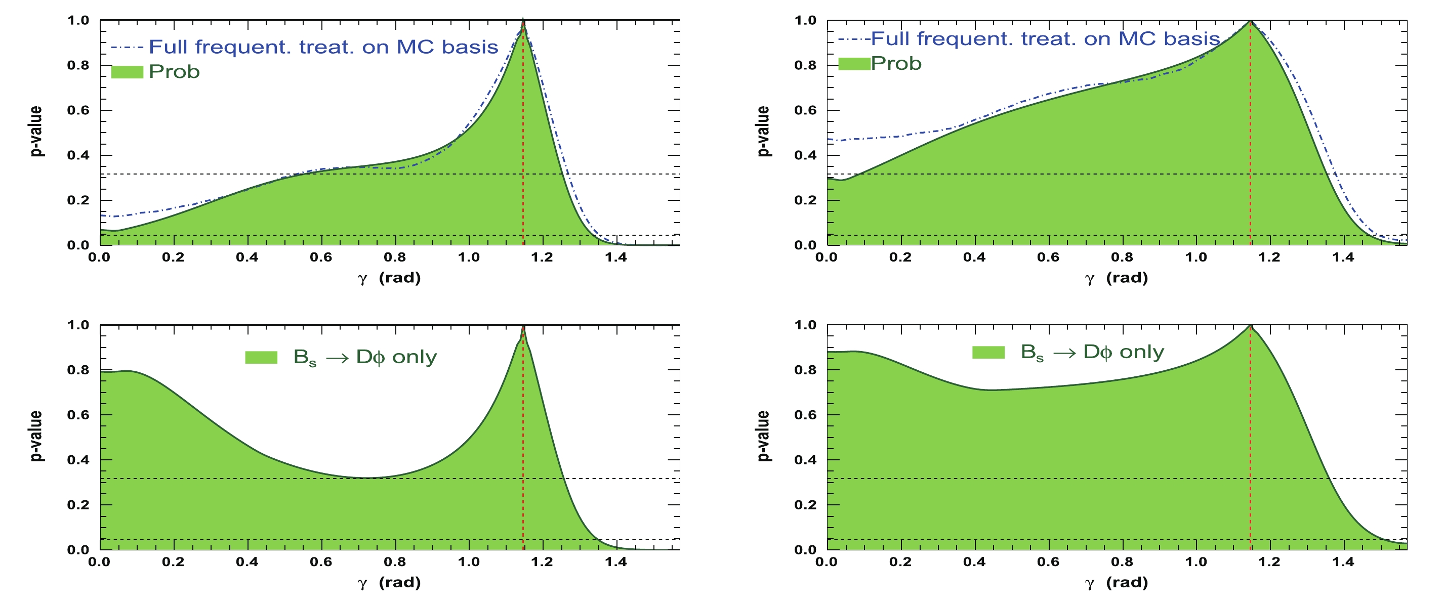
Figure 3. (color online) Profile of p-value of global
$\chi^2$ fit to$\gamma$ after computing observables (top left) for a set of true initial parameters:$\gamma=1.146$ rad,${r^{(*)}_{B}}=0.4$ ,${\delta_{B}}=3.0$ rad, and${\delta^*_{B}}=2.0$ rad (the corresponding distribution obtained from the full frequentist treatment on the Monte-Carlo simulation basis [50] is superimposed on the same distribution). The related p-value profile for${r^{(*)}_{B}}=0.22$ is also presented (top right). The assumed integrated luminosity assumed is that of the LHCb data collected in Run 1 & 2. Profile of p-value of global$\chi^2$ fit to$\gamma$ after computing observables, where only decay mode${B^0_s}\rightarrow \tilde{D}^0\phi$ is used, and for a set of true initial parameters:$\gamma=1.146$ rad,${r^{(*)}_{B}}=0.4$ (bottom left) and$0.22$ (bottom right),${\delta_{B}}=3.0$ rad, and${\delta^*_{B}}=2.0$ rad. In each figure, the vertical dashed red line indicates the initial$\gamma$ true value, and the two horizontal dashed black lines refer to 68.3 and 95.4% CLs.Figure 4 displays the 1-D p-value profile of the nuisance parameters
$r^{(*)}_B $ and$\delta^{(*)}_B $ for the same set of initial parameters ($ \gamma = 65.66^{\circ} $ (1.146 rad),$ {{r^{(*)}_{B}}} = 0.4 $ ,$ {{\delta_{B}}} = 3.0 $ rad, and$ {{\delta^*_{B}}} = 2.0 $ rad) and the same projected integrated luminosity. It can be observed that the p-value is the maximum at the initial tested value, as expected.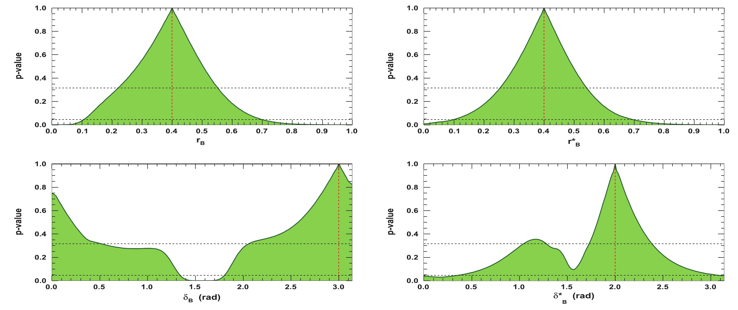
Figure 4. (color online) Profiles of p-value distributions of global
$\chi^2$ fit to${r^{(*)}_{B}}$ (top left (right)) and$\delta _B^{(*)}$ (bottom left (right)) after computing observables for set of initial true parameters:$\gamma=65.66^{\circ}$ (1.146 rad),${r^{(*)}_{B}}=0.4$ ,${\delta_{B}}=3.0$ rad, and${\delta^*_{B}}=2.0$ rad. In each figure, thevertical dashed red line indicates the initial${r^{(*)}_{B}}$ and$\delta _B^{(*)}$ true values, and the two horizontal dashed black lines refer to 68.3 and 95.4% CLs.The 2-D p-value profiles of the nuisance parameters
$ {{r^{(*)}_{B}}} $ and$ {{\delta^{(*)}_{B}}} $ as a function of$ \gamma $ are presented in Figs. 5-8. Figures 5 and 6 correspond to two other example configurations$ \gamma = 1.146 $ rad,$ {{\delta_{B}}} = 1.0 $ rad, and$ {{\delta^*_{B}}} = 5.0 $ rad, and$ {{r^{(*)}_{B}}} = 0.4 $ and$ {{r^{(*)}_{B}}} = 0.22 $ , respectively. Figures 7 and 8 represent the configurations$ \gamma = 1.146 $ rad,$ {{\delta_{B}}} = 3.0 $ rad, and$ {{\delta^*_{B}}} = 2.0 $ rad, and$ {{r^{(*)}_{B}}} = 0.4 $ and$ {{r^{(*)}_{B}}} = 0.22 $ , respectively. These 2-D views allow the correlation between the different parameters to be observed. In general, large correlations between$ \delta^{(*)}_{B} $ and$ \gamma $ are observed. In the case of configurations where$ {{r^{(*)}_{B}}} = 0.4 $ , a large fraction of the$ {{\delta^{(*)}_{B}}} $ vs.$ \gamma $ plane can be excluded at a$ 95 $ % CL, whereas the fraction is significantly reduced for the corresponding$ {{r^{(*)}_{B}}} = 0.22 $ configurations. For the$ {{\delta^*_{B}}} $ vs.$ \gamma $ plane, the advantage of our Cartesian coordinate approach (see Section IIB and IIC) can easily be observed, together with the fact that in the case of the mode$ {{D^{*0}}} \rightarrow {{D^0}} \gamma $ , there is an effective strong phase shift of$ \pi $ with respect to the$ {{D^{*0}}} \rightarrow {{D^0}} \pi^{0} $ [37], such that additional constraints enable the fold ambiguities with respect to the associated$ {{\delta_{B}}} $ vs.$ \gamma $ plane to be removed.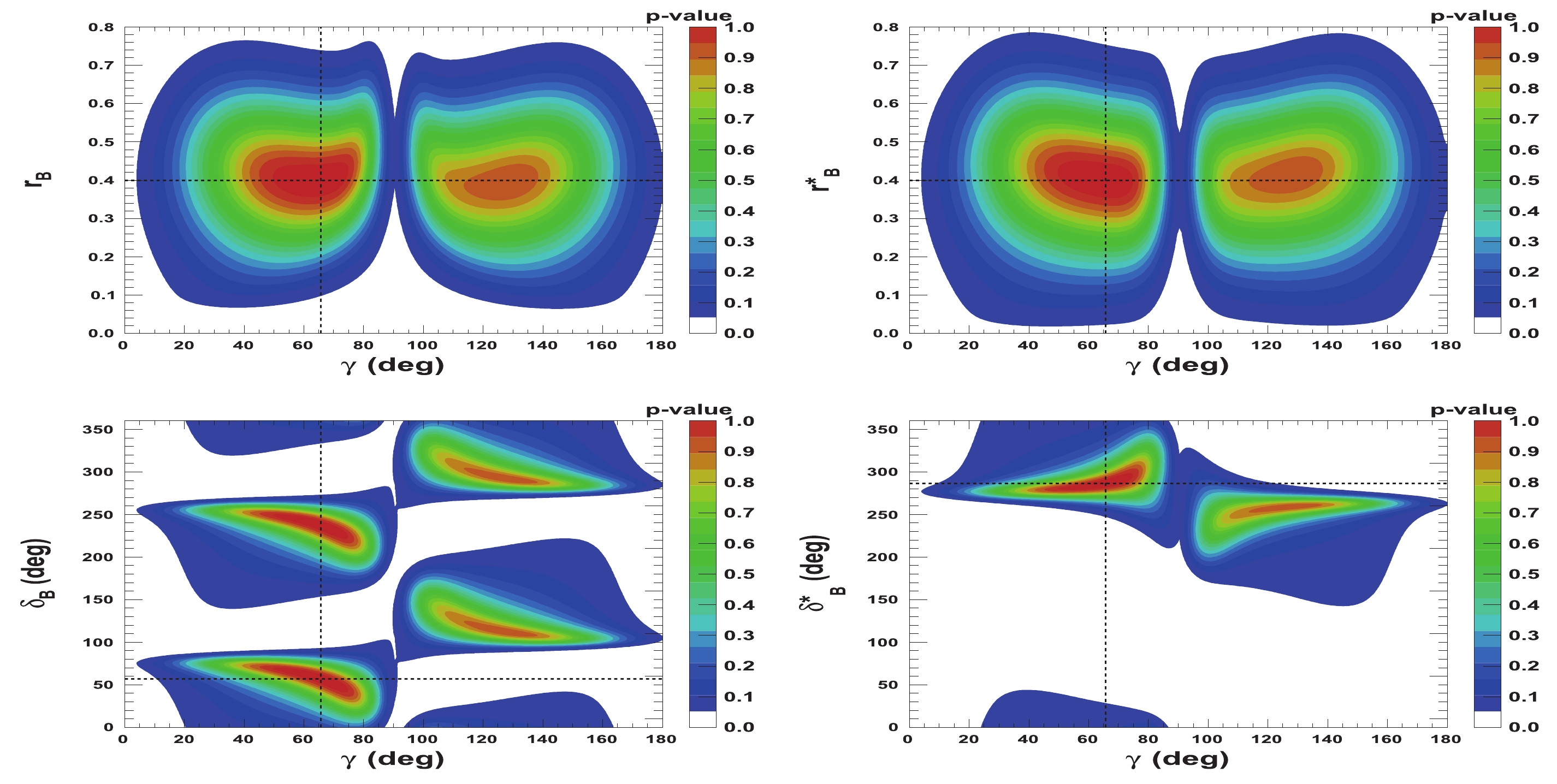
Figure 5. (color online) 2-D p-value profile distribution of nuisance parameters
${r^{(*)}_{B}}$ and$\delta _B^{(*)}$ as a function of$\gamma$ . In each figure, the dashed black lines indicate the initial true values:$\gamma=65.66^\circ$ (1.146 rad),${\delta_{B}}=57.3^\circ$ (1.0 rad), and${\delta^*_{B}}=286.5^\circ$ (5.0 rad), as well as${r^{(*)}_{B}}=0.4$ .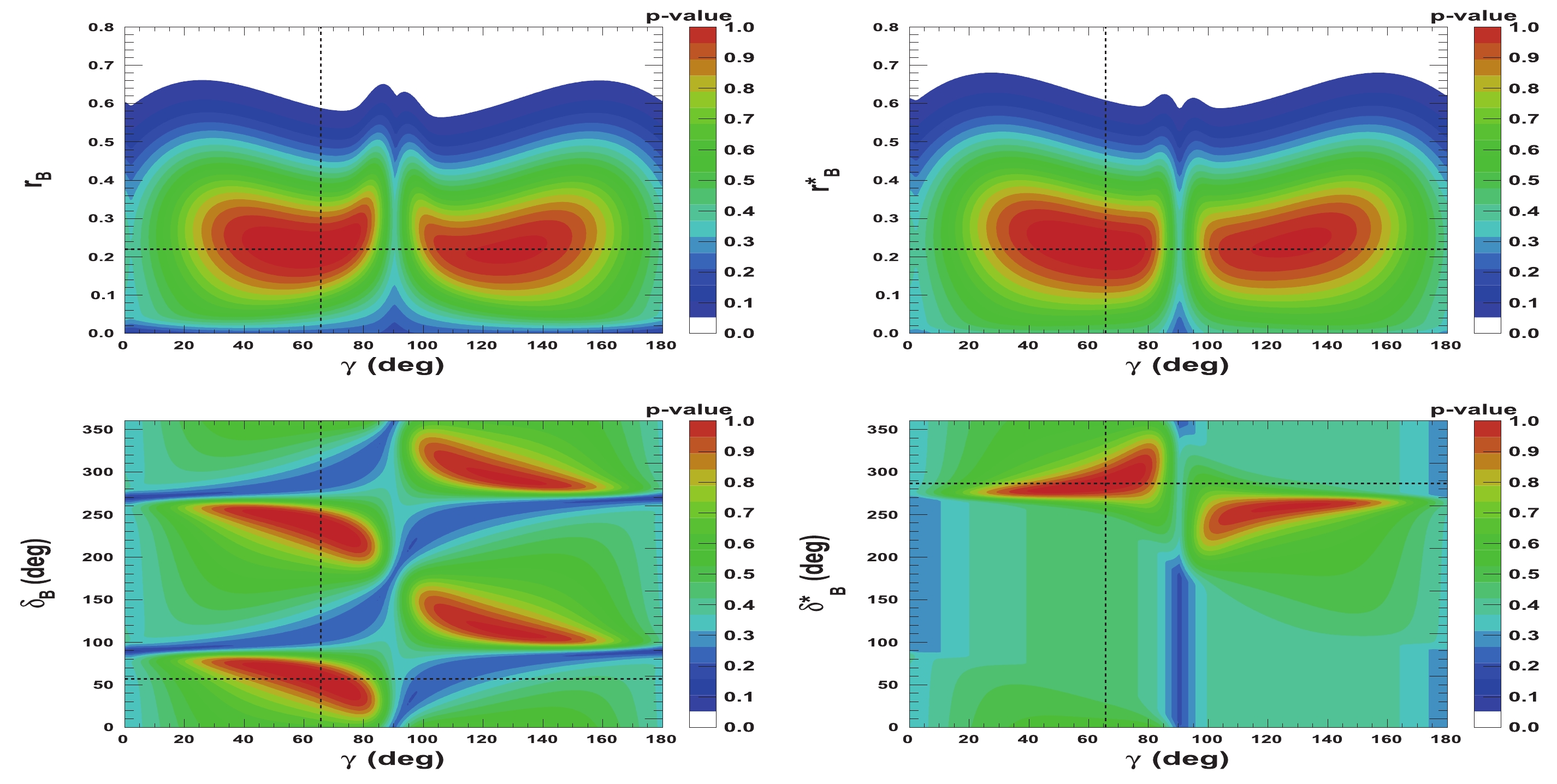
Figure 6. (color online) 2-D p-value profile distribution of nuisance parameters
${r^{(*)}_{B}}$ and$\delta _B^{(*)}$ as a function of$\gamma$ . In each figure, the dashed black lines indicate the initial true values:$\gamma=65.66^\circ$ (1.146 rad),${\delta_{B}}=57.3^\circ$ (1.0 rad), and${\delta^*_{B}}=286.5^\circ$ (5.0 rad), as well as${r^{(*)}_{B}}=0.22$ .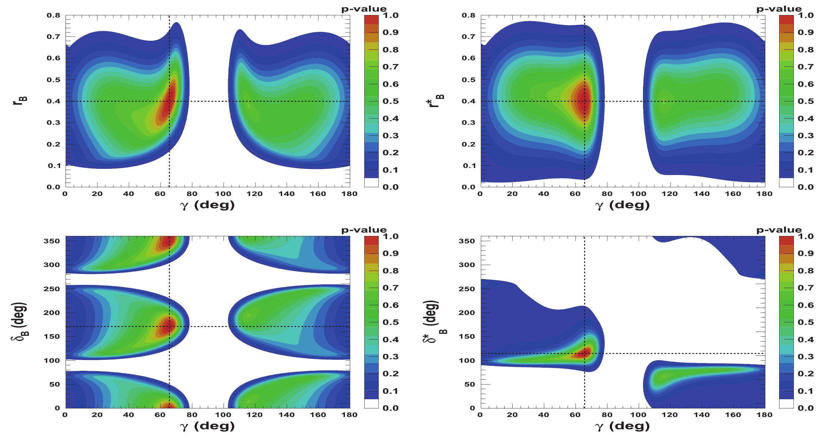
Figure 7. (color online) 2-D p-value profile distribution of nuisance parameters
${r^{(*)}_{B}}$ and$\delta _B^{(*)}$ as a function of$\gamma$ . In each figure, the dashed black lines indicate the initial true values:$\gamma=65.66^\circ$ (1.146 rad),${\delta_{B}}=171.9^\circ$ (3.0 rad), and${\delta^*_{B}}=114.6^\circ$ (2.0 rad), as well as${r^{(*)}_{B}}=0.4$ .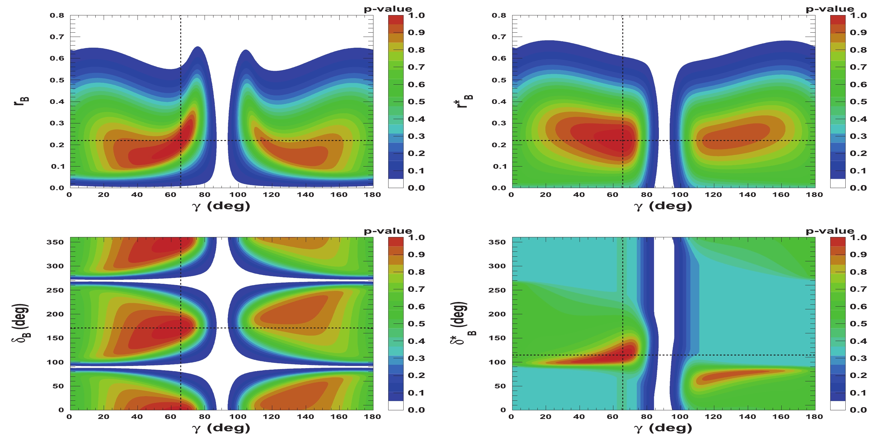
Figure 8. (color online) 2-D p-value profile distribution of nuisance parameters
${r^{(*)}_{B}}$ and$\delta _B^{(*)}$ as a function of$\gamma$ . In each figure, the dashed black lines indicate the true values:$\gamma=65.66^\circ$ (1.146 rad),${\delta_{B}}=171.9^\circ$ (3.0 rad), and${\delta^*_{B}}=114.6^\circ$ (2.0 rad), as well as${r^{(*)}_{B}}=0.22$ . -
Figure 9 demonstrates that for a tested configuration of
$ \gamma = 1.146 $ rad,$ {{r^{(*)}_{B}}} = 0.4 $ , and$ {{\delta^{(*)}_{B}}} = 1.0 $ rad, the impact of the time acceptance parameters$ {\cal{A}} $ and$ {\cal{B}} $ can eventually be non negligible and the parameters affect the profile distribution of the p-value of the global$ \chi^2 $ fit to$ \gamma $ . For the given example, the fitted value of$ \gamma $ is either$ \left(65.3^{+14.3}_{-38.4}\right)^\circ $ or$ \left(66.5^{+13.8}_{-51.0}\right)^\circ $ when the time acceptance is either accounted for or not. The reason due to which the precision improves when the time acceptance is taken into account may not be intuitive. This is because, for$ {\cal{B}}/{\cal{A}}\simeq1.6 $ , as opposed to the case of$ {\cal{B}}/{\cal{A}}\simeq1.0 $ , the impact of the first term in Eq. (14), which is directly proportional to$ \cos \left({{\delta_{B}}} + 2\beta_{s} - \gamma \right) $ , is amplified with respect to the second term, for which the sensitivity to$ \gamma $ is more diluted.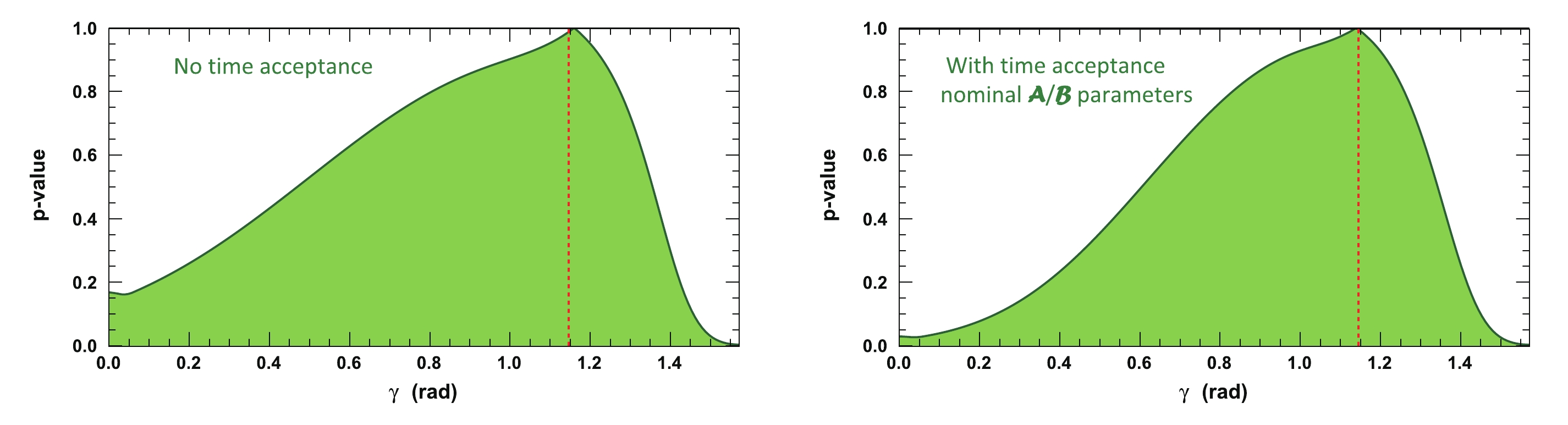
Figure 9. (color online) Profile of p-value distribution of global
$\chi^2$ fit to$\gamma$ for a set of true initial parameters:$\gamma=1.146$ rad,${r^{(*)}_{B}}=0.4$ , and$\delta _B^{(*)}=1.0$ rad. The assumed integrated luminosity is that of the LHCb data collected in Run 1 & 2 when the time acceptance values${\cal{A}}$ and${\cal{B}}$ are set to 1 in Eqs. (14) to (34): no time acceptance (top left) or to their nominal values${\cal{A}}=0.488\pm 0.005$ and${\cal{B}}=0.773\pm 0.008$ (top right), as computed in Section IIA. The dashed red line indicates the initial$\gamma$ true value$\gamma=65.66^\circ$ (1.146 rad).Even if the parameters
$ {\cal{A}} $ and$ {\cal{B}} $ are computed to a precision at the percentage level (Section IIA), we further investigate the effect of changing their values. Note that for this study, the overall efficiency is maintained constant, whereas the shape of the acceptance function is varied. The values$ \alpha $ ,$ \beta $ , and$ \xi $ are changed in Eq. (10), and the results of those changes are listed in Table 4. When$ \alpha $ increases, both$ {\cal{A}} $ and$ {\cal{B}} $ become larger, but the value of the ratio$ {\cal{B}}/{\cal{A}} $ decreases. When$ \beta $ or$ \xi $ decreases, the three values of$ {\cal{A}} $ ,$ {\cal{B}} $ , and$ {\cal{B}}/{\cal{A}} $ increase. The effect of changing$ \beta $ or$ \xi $ alone is small. A modification of$ \alpha $ has a much greater impact on$ {\cal{A}} $ and$ {\cal{B}} $ . However, all of these changes have a weak impact on the precision of the fitted$ \gamma $ value. This is quite encouraging, as it means that the relative efficiency loss caused by the time acceptance effects will not cause a significant change in the sensitivity to the CKM$ \gamma $ angle. As a result, the time acceptance requirements can be varied without substantial concern to improve the signal purity and statistical significance when analyzing the$ {{B^0_s}}\rightarrow \tilde{D}^{(*)0}\phi $ decays with LHCb data.$ \alpha $ 

$ \beta $ 

$ \xi $ 

$ {\cal{A}} $ 

$ {\cal{B}} $ 

$ {\cal{B}}/{\cal{A}} $ 

Fitted $ \gamma $ (

$ ^{\circ} $ )

1.0 2.5 0.01 0.367 0.671 1.828 $ 66.5^{+13.8}_{-40.1} $ 

1.5 2.5 0.01 0.488 0.773 1.584 $ {\bf{{ 65.3^{+14.3}_{-38.4}}}} $ 

2.0 2.5 0.01 0.570 0.851 1.493 $ 65.3^{+13.2}_{-37.8} $ 

1.5 2.0 0.01 0.484 0.751 1.552 $ 65.9^{+13.2}_{-39.0} $ 

1.5 3.0 0.01 0.491 0.789 1.607 $ 66.5^{+13.2}_{-38.4} $ 

1.5 2.5 0.02 0.480 0.755 1.573 $ 66.5^{+13.8}_{-39.5} $ 

1.5 2.5 0.005 0.492 0.783 1.591 $ 65.3^{+13.8}_{-36.7} $ 

Table 4. Expected value of
$ \gamma $ as a function of different time acceptance parameters. The second line corresponds to the nominal values. The nominal set of parameters$ {\cal{A}} $ and$ {\cal{B}} $ is indicated in bold. -
According to Ref. [46], the averaged values of the
$ K3\pi $ input parameters over the phase space, which are defined as$ R^{K3\pi}_D {\rm e}^{-{\rm i}\delta^{K3\pi}_{D}} = \frac{\int A^*_{{{\bar{D}^0}} \rightarrow K3\pi}(x)A_{{{D^0}} \rightarrow K3\pi}(x) {\rm d}x}{A_{{{\bar{D}^0}} \rightarrow K3\pi}A_{{{D^0}} \rightarrow K3\pi}}, $

(35) are used here and correspond to a relatively limited value for the coherence factor:
$ R^{K3\pi}_D = (43^{+17}_{-13}) $ % [36]. A more attractive approach may be to perform the analysis in disjoint bins of the phase space. In this case, the parameters are re-defined within each bin. New values for$ R^{K3\pi}_D $ and$ \delta^{K3\pi}_{D} $ in each bin from Ref. [52] have alternatively been employed. No noticeable changes were observed in the$ \gamma $ and$ {{r^{(*)}_{B}}} $ fitted p-value profiles, but it is possible that certain fold-effects on$ {{\delta^{(*)}_{B}}} $ , e.g., as observed in Figs. 5-7, become less probable. The lack of significant improvement is expected as the$ {{\tilde{D}^0}} \rightarrow K3\pi $ mode is not the dominant decay, and also because the new measurements of$ R^{K3\pi}_{D} $ and$ \delta^{K3\pi}_{D} $ in each bin still have large uncertainties. -
As explained in Section IVB, for each of the tested
$ \gamma $ ,$ {{r^{(*)}_{B}}} $ , and$ {{\delta^{(*)}_{B}}} $ configurations, 4000 pseudoexperiments are generated, for which the values of$ \gamma $ ,$ {{r^{(*)}_{B}}} $ , and$ {{\delta^{(*)}_{B}}} $ are unfolded from the global$ \chi^2 $ fits (see Section IVC for illustrations). Figure 10 displays the extended unbinned maximum likelihood fits to the nuisance parameters$ {{r^{(*)}_{B}}} $ and$ {{\delta^{(*)}_{B}}} $ . The initial configuration is$ \gamma = 65.66^{\circ} $ (1.146 rad),$ {{r^{(*)}_{B}}} = 0.4 $ ,$ {{\delta_{B}}} = 171.9^\circ $ (3 rad), and$ {{\delta^*_{B}}} = 114.6^\circ $ (2 rad), with an integrated luminosity that is equivalent to that of the LHCb Run 1 & 2 data. It can be compared with Fig. 4. All of the distributions are fitted with the Novosibirsk empirical function, the description of which contains a Gaussian core part and a left or right tail, depending on the sign of the tail parameter [53]. The fitted values of$ {{r^{(*)}_{B}}} $ are centered at their initial tested values of 0.4, with a resolution of 0.14, and no bias is observed. For$ {{\delta^{(*)}_{B}}} $ , the fitted value is$ (176\pm42)^\circ $ ($ (104\pm13)^\circ $ ) for an initial true value that is equal to$ 171.9^\circ $ ($ 114.6^\circ $ ). The fitted value for$ {{\delta^*_{B}}} $ is slightly shifted by approximately$ 2/3 $ of a standard deviation, but its measurement is much more precise than that of$ {{\delta_{B}}} $ , as it is measured from both the$ {{D^{*0}}} \rightarrow {{D^0}} \gamma $ and$ {{D^{*0}}} \rightarrow {{D^0}} \pi^{0} $ observables.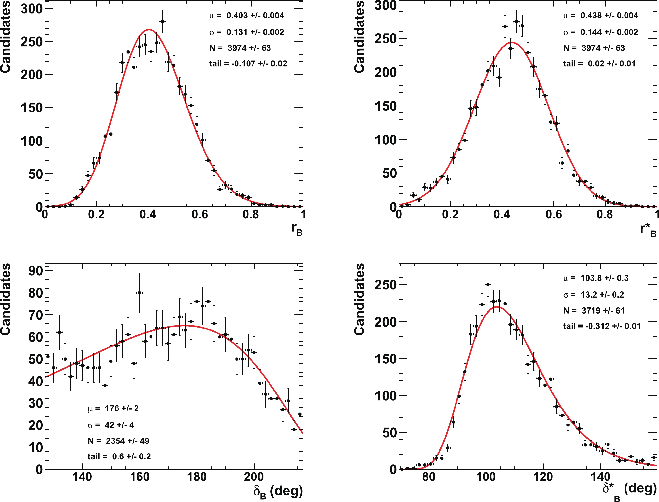
Figure 10. (color online) Fit to distributions of nuisance parameters
${r^{(*)}_{B}}$ (top left (right)) and$\delta _B^{(*)}$ (bottom left (right)) obtained from 4000 pseudoexperiments. The initial configuration is$\gamma=65.66^{\circ}$ (1.146 rad),${r^{(*)}_{B}}=0.4$ ,${\delta_{B}}=171.9^\circ$ (3 rad), and${\delta^*_{B}}=114.6^\circ$ (2 rad). The distributions of$\delta _B^{(*)}$ are plotted and fitted within$\pm 45^\circ$ of their initial true values. In the distributions, only the candidates with values of$\gamma\ \in \ [0^\circ, \ 90^\circ]$ are considered.Figure 11 presents the corresponding fit to the CKM angle
$ \gamma $ , where the value$ {{r^{(*)}_{B}}} = 0.22 $ is also tested. This figure can be compared to the initial p-value profiles illustrated in Fig. 3. As shown in Figs. 7 and 8,$ \gamma $ is correlated with the nuisance parameters$ {{r^{(*)}_{B}}} $ and$ {{\delta^{(*)}_{B}}} $ . Such correlations may generate long tails in the distributions, as obtained from the 4000 pseudoexperiments. To account for these tails, extended unbinned maximum likelihood fits, constituting two Novosibirsk functions with opposite-side tails, are performed on the$ \gamma $ distributions. With an initial value of$ 65.66^\circ $ , the fitted value for$ \gamma $ returns a central value equal to$ \mu_{\gamma} = (65.9\pm0.3)^\circ $ with a resolution of$ \sigma_{\gamma} = (8.8\pm0.2)^\circ $ when$ {{r^{(*)}_{B}}} = 0.4 $ , and$ \mu_{\gamma} = (66.6\pm0.7)^\circ $ with a resolution of$ \sigma_{\gamma} = (14.4\pm0.5)^\circ $ when$ {{r^{(*)}_{B}}} = 0.22 $ . The worse resolution obtained with$ {{r^{(*)}_{B}}} = 0.22 $ follows the empirical behavior$ 1/{{r^{(*)}_{B}}} $ ($ 8.8\times0.4/0.22\simeq 16.0 $ ). Again, no bias is observed.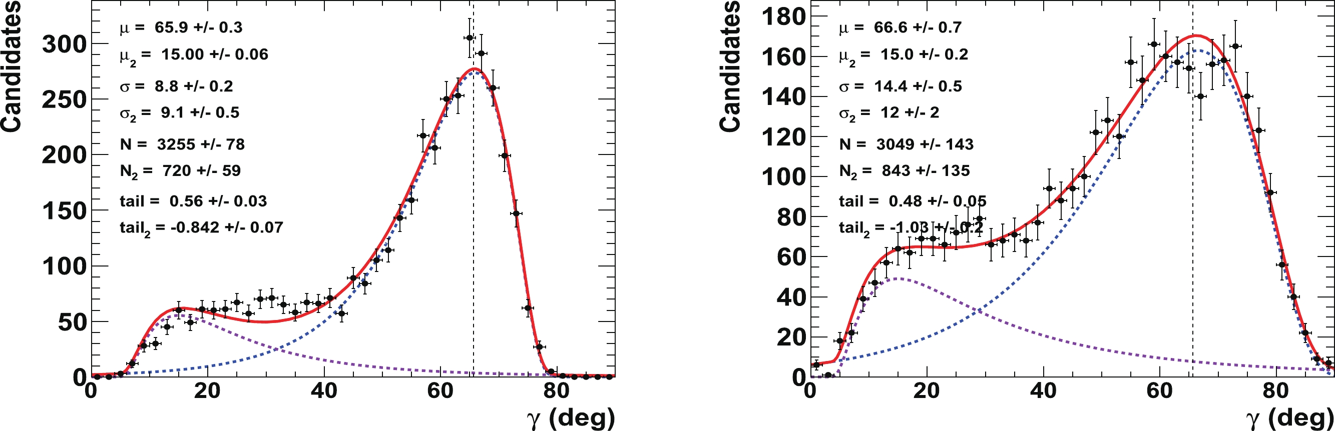
Figure 11. (color online) Fit to distributions of nuisance parameters
$\gamma$ obtained from 4000 pseudoexperiments. The initial configuration is$\gamma=65.66^{\circ}$ (1.146 rad),${r^{(*)}_{B}}=0.4$ (left) and 0.22 (right),${\delta_{B}}=171.9^\circ$ (3 rad), and${\delta^*_{B}}=114.6^\circ$ (2 rad). In the distributions, only the candidates with a value of$\gamma\ \in \ [0^\circ, \ 90^\circ]$ are considered. The purple dashed curve represents tails generated by the correlations with the nuisance parameters${r^{(*)}_{B}}$ and$\delta _B^{(*)}$ , whereas the blue dashed curve indicates the core part of the distribution, and the plain red line is the sum of the two components of the fit.Finally, Fig. 12 displays the 2-D distributions of the nuisance parameters
$ {{r^{(*)}_{B}}} $ and$ {{\delta^{(*)}_{B}}} $ as a function of$ \gamma $ obtained from 4000 pseudoexperiments. This figure can be compared with the corresponding p-value profiles presented in Fig. 7.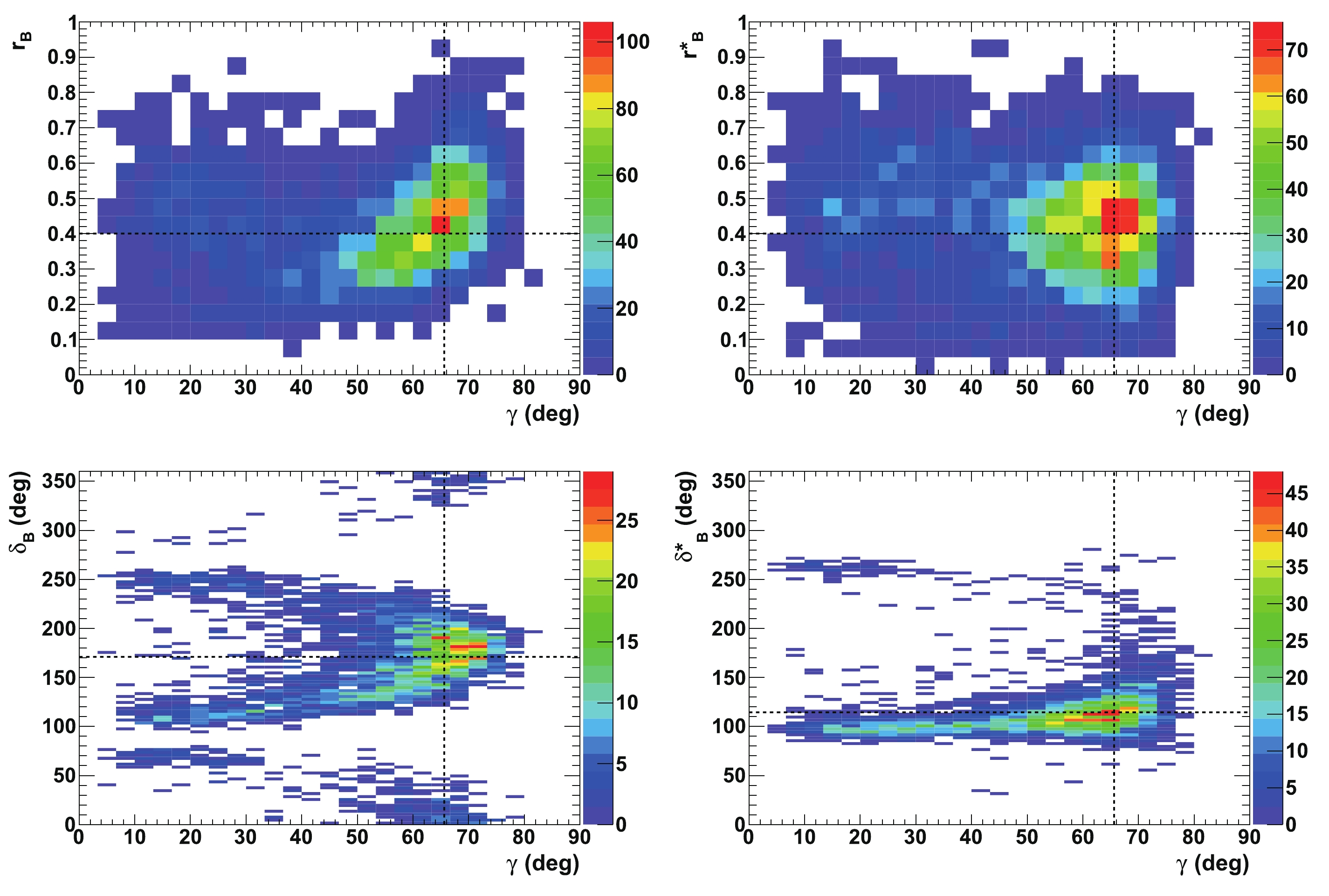
Figure 12. (color online) 2-D distributions of nuisance parameters
${r^{(*)}_{B}}$ and$\delta _B^{(*)}$ as a function of$\gamma$ obtained from 4000 pseudoexperiments. In each figure, the horizontal dashed black lines indicate the initial true values:$\gamma=65.66^\circ$ (1.146 rad),${\delta_{B}}=171.9^\circ$ (3.0 rad), and${\delta^*_{B}}=114.6^\circ$ (2.0 rad), as well as${r^{(*)}_{B}}=0.4$ . -
According to Section IVA, 72 configurations of nuisance parameters
$ {{\delta^{(*)}_{B}}} $ and$ {{r^{(*)}_{B}}} $ have been tested for$ \gamma = 65.66^\circ $ (1.146 rad) and 4000 pseudoexperiments have been generated for each set, following the procedure described in Section IVB and illustrated in Section IVF. The assumed integrated luminosity in this section is that of the LHCb data collected in Run 1 & 2.The fitted mean values of
$ \gamma $ ($ \mu_{\gamma} $ ) for$ {{r^{(*)}_{B}}} = 0.4 $ and$ 0.22 $ as a function of$ {{\delta^{(*)}_{B}}} $ , for an initial true value of$ 65.66^\circ $ (1.146 rad), are displayed in Table 5, whereas the corresponding resolutions ($ \sigma_{\gamma} $ ) are listed in Table 6. In general, the fitted means are compatible with the true$ \gamma $ values within less than one standard deviation. For$ {{r^{(*)}_{B}}} = 0.4 $ , the resolution varies from$ \sigma_{\gamma} = 8.3^\circ $ to$ 12.9^\circ $ . For$ {{r^{(*)}_{B}}} = 0.22 $ , the resolution is worse, as expected, and it varies from$ \sigma_{\gamma} = 13.9^\circ $ to$ 18.7^\circ $ . For$ {{r^{(*)}_{B}}} = 0.22 $ , the distribution of$ \gamma $ of the 4000 pseudoexperiments has its maximum above$ 90^\circ $ for$ {{\delta^{(*)}_{B}}} = 286.5^\circ $ and it is therefore not considered.$ {{\delta_{B}}} $ 

$ {{\delta^*_{B}}} $ 

0 57.3 114.6 171.9 229.2 286.5 $ {{r^{(*)}_{B}}}=0.4 $ 

0.0 $ 66.2 \pm0.4 $ 

$ 65.9 \pm0.4 $ 

$ 67.4 \pm0.4 $ 

$ 65.9 \pm0.4 $ 

$ 65.9 \pm0.4 $ 

$ 67.4 \pm0.4 $ 

57.3 $ 65.4 \pm0.4 $ 

$ 69.2 \pm0.4 $ 

$ 71.4 \pm0.4 $ 

$ 65.5 \pm0.3 $ 

$ 67.7 \pm0.4 $ 

$ 72.6 \pm0.4 $ 

114.6 $ 65.8 \pm0.4 $ 

$ 70.5 \pm0.4 $ 

$ 72.9 \pm0.4 $ 

$ 65.9 \pm0.3 $ 

$ 69.3 \pm0.4 $ 

$ 73.8 \pm0.4 $ 

171.9 $ 65.6_{-0.4}^{+0.5} $ 

$ 65.2 \pm0.3 $ 

$ 65.9 \pm0.3 $ 

$ 65.5 \pm0.3 $ 

$ 65.2 \pm0.4 $ 

$ 66.1 \pm0.3 $ 

229.2 $ 64.9 \pm0.4 $ 

$ 67.6 \pm0.4 $ 

$ 68.9 \pm0.4 $ 

$ 65.0 \pm0.4 $ 

$ 67.1 \pm0.4 $ 

$ 69.0 \pm0.4 $ 

286.5 $ 66.1 \pm0.4 $ 

$ 71.0 \pm0.4 $ 

$ 75.7 \pm0.4 $ 

$ 65.7 \pm0.3 $ 

$ 69.8 \pm0.4 $ 

$ 78.8 \pm0.4 $ 

$ {{\delta_{B}}} $ 

$ {{\delta^*_{B}}} $ 

0 57.3 114.6 171.9 229.2 286.5 $ {{r^{(*)}_{B}}}=0.22 $ 

0.0 $ 67.2_{-1.0}^{+0.9} $ 

$ 68.1_{-0.9}^{+1.0} $ 

$ 68.3_{-0.8}^{+0.9} $ 

$ 67.1 \pm0.8 $ 

$ 68.4 \pm0.9 $ 

$ 69.0 \pm0.8 $ 

57.3 $ 67.4 \pm0.9 $ 

$ 72.2 \pm0.8 $ 

$ 74.1_{-0.7}^{+0.8} $ 

$ 66.6 \pm0.7 $ 

$ 71.5 \pm0.8 $ 

$ 75.5 \pm0.8 $ 

114.6 $ 65.7 \pm0.9 $ 

$ 71.8 \pm0.6 $ 

$ 74.9 \pm0.6 $ 

$ 68.0 \pm0.6 $ 

$ 71.2 \pm0.7 $ 

$ 74.9 \pm0.6 $ 

117.9 $ 65.4 \pm0.7 $ 

$ 66.9 \pm0.7 $ 

$ 66.6 \pm0.7 $ 

$ 64.7 \pm0.7 $ 

$ 65.2 \pm0.6 $ 

$ 68.3 \pm0.6 $ 

229.2 $ 65.9_{-1.0}^{+0.9} $ 

$ 69.1 \pm0.8 $ 

$ 70.1_{-0.8}^{+0.7} $ 

$ 67.7 \pm0.7 $ 

$ 67.4 \pm0.7 $ 

$ 71.0_{-0.7}^{+0.6} $ 

286.5 $ 67.5 \pm0.9 $ 

$ 75.8 \pm0.8 $ 

$ 77.5_{-0.7}^{+0.8} $ 

$ 68.1 \pm0.6 $ 

$ 72.8_{-0.8}^{+0.9} $ 

$ 83.5_{-1.5}^{+2.4} $ 

Table 5. Fitted mean values of
$ \gamma $ ($ \mu_{\gamma} $ ) (in [deg]) for$ {{r^{(*)}_{B}}} = 0.4 $ (top) and$ 0.22 $ (bottom), as a function of$ {{\delta^{(*)}_{B}}} $ , for initial true value of$ 65.66^\circ $ .$ {{\delta_{B}}} $ 

$ {{\delta^*_{B}}} $ 

0 57.3 114.6 171.9 229.2 286.5 $ {{r^{(*)}_{B}}}=0.4 $ 

0.0 $ 9.6 \pm0.4 $ 

$ 11.2 \pm0.3 $ 

$ 11.2 \pm0.3 $ 

$ 9.4 \pm0.4 $ 

$ 12.2 \pm0.4 $ 

$ 11.2 \pm0.3 $ 

57.3 $ 11.2 \pm0.3 $ 

$ 12.6 \pm0.3 $ 

$ 11.8 \pm0.3 $ 

$ 10.2 \pm0.3 $ 

$ 12.4 \pm0.3 $ 

$ 12.9 \pm0.3 $ 

114.6 $ 11.4 \pm0.3 $ 

$ 11.9 \pm0.3 $ 

$ 11.1 \pm0.3 $ 

$ 10.0 \pm0.3 $ 

$ 11.3 \pm0.3 $ 

$ 11.9 \pm0.3 $ 

171.9 $ 8.3 \pm0.4 $ 

$ 9.8 \pm0.3 $ 

$ 8.8 \pm0.2 $ 

$ 8.9 \pm0.3 $ 

$ 9.5 \pm0.3 $ 

$ 9.0 \pm0.2 $ 

229.2 $ 10.8 \pm0.3 $ 

$ 11.7 \pm0.3 $ 

$ 10.8 \pm0.3 $ 

$ 10.3 \pm0.3 $ 

$ 12.4 \pm0.3 $ 

$ 11.7 \pm0.3 $ 

286.5 $ 11.0 \pm0.3 $ 

$ 12.9 \pm0.3 $ 

$ 11.6 \pm0.3 $ 

$ 9.2 \pm0.2 $ 

$ 11.7 \pm0.3 $ 

$ 13.2_{-0.5}^{+0.6} $ 

$ {{\delta_{B}}} $ 

$ {{\delta^*_{B}}} $ 

0 57.3 114.6 171.9 229.2 286.5 $ {{r^{(*)}_{B}}}=0.22 $ 

0.0 $ 16.5 \pm0.7 $ 

$ 16.8 \pm0.7 $ 

$ 16.0 \pm0.6 $ 

$ 16.8_{-0.7}^{+0.8} $ 

$ 15.9_{-0.6}^{+0.0} $ 

$ 16.0 \pm0.7 $ 

57.3 $ 16.7 \pm0.6 $ 

$ 18.1_{-0.8}^{+0.9} $ 

$ 17.1_{-0.9}^{+1.0} $ 

$ 14.3 \pm0.5 $ 

$ 16.8 \pm0.7 $ 

$ 17.6_{-1.1}^{+1.3} $ 

114.6 $ 16.1_{-0.7}^{+0.6} $ 

$ 15.9 \pm0.6 $ 

$ 13.9 \pm0.5 $ 

$ 14.1 \pm0.5 $ 

$ 15.1 \pm0.6 $ 

$ 14.9 \pm0.6 $ 

171.9 $ 15.7_{-0.6}^{+0.7} $ 

$ 14.5 \pm0.5 $ 

$ 14.4 \pm0.5 $ 

$ 15.5 \pm0.6 $ 

$ 15.7_{-0.5}^{+0.0} $ 

$ 14.0 \pm0.5 $ 

229.2 $ 15.9 \pm0.6 $ 

$ 15.7_{-0.6}^{+0.5} $ 

$ 15.4 \pm0.6 $ 

$ 14.6_{-0.5}^{+0.6} $ 

$ 15.6 \pm0.5 $ 

$ 14.4 \pm0.6 $ 

286.5 $ 16.9_{-0.6}^{+0.7} $ 

$ 18.0_{-1.1}^{+1.3} $ 

$ 16.7_{-1.0}^{+1.2} $ 

$ 14.9_{-0.6}^{+0.5} $ 

$ 16.1 \pm0.7 $ 

$ 18.7_{-2.1}^{+2.8} $ 

Table 6. Fitted resolution of
$ \gamma $ ($ \sigma_{\gamma} $ ) (in [deg]) for$ {{r^{(*)}_{B}}} = 0.4 $ (top) and$ 0.22 $ (bottom), as a function of$ {{\delta^{(*)}_{B}}} $ .The obtained values for
$ \mu_{\gamma} $ and$ \sigma_{\gamma} $ are also displayed in Figs. 13 and 14. It is clear that the resolution on$ \gamma $ depends to the first order on$ {{r^{(*)}_{B}}} $ , and then to the second order on$ {{\delta^{(*)}_{B}}} $ . The best agreement with respect to the tested initial true value of$ \gamma $ is obtained when$ {{\delta^{(*)}_{B}}} = 0^\circ $ (0 rad) or$ 180^\circ $ ($ \pi $ rad), and the best resolutions (the lowest values of$ \sigma_{\gamma} $ ) are also obtained in this case. The largest CP violation effects and best sensitivity to$ \gamma $ are observed. In contrast, the worst sensitivity is obtained when$ {{\delta^{(*)}_{B}}} = 90^\circ $ ($ \pi/2 $ rad) or$ 270^\circ $ ($ 3\pi/2 $ rad). The other best and worst positions for$ {{\delta^{(*)}_{B}}} $ can easily be deduced from Eq. (14). In most cases, for$ {{r^{(*)}_{B}}} = 0.4 $ (0.22), the value of the resolution is$ \sigma_{\gamma}\sim10^\circ $ ($ 15^\circ $ ) and the fitted mean value$ \mu_{\gamma} \sim 65.66^\circ $ or slightly larger.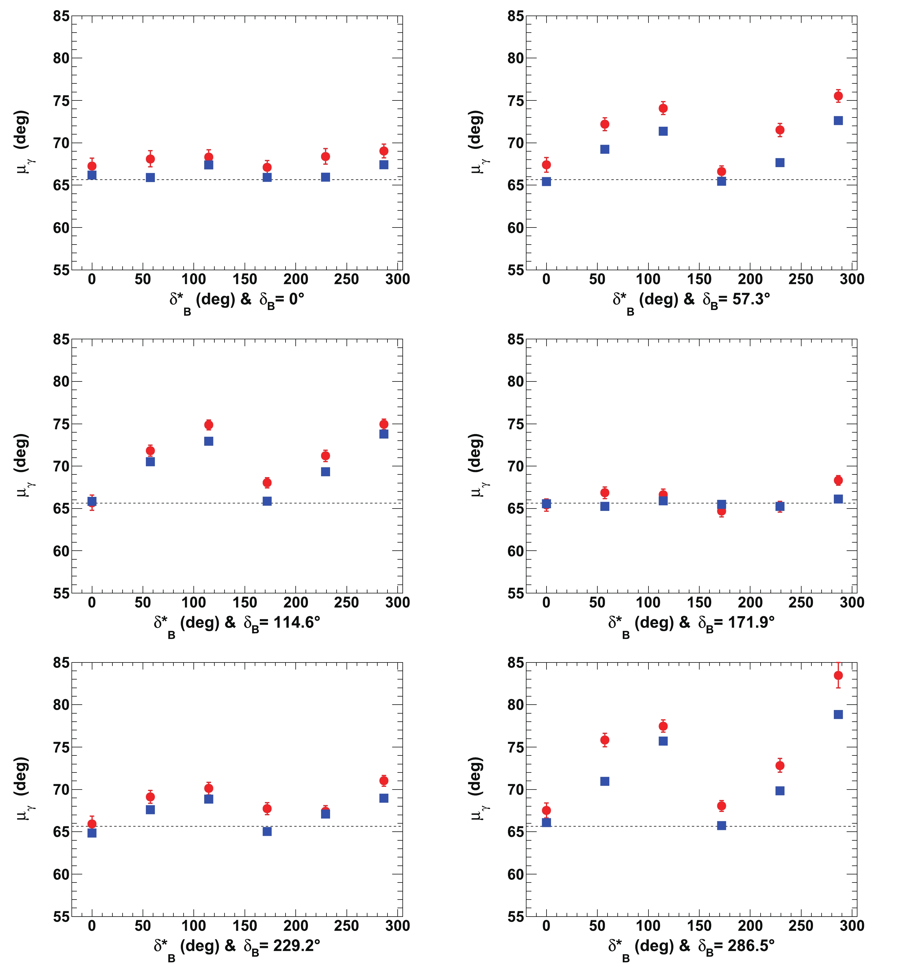
Figure 13. (color online) Fitted mean values of
$\gamma$ ($\mu_{\gamma}$ ) for${r^{(*)}_{B}}=0.22$ (red circles) and 0.4 (blue squares) as a function of$\delta _B^{(*)}$ for initial true value of$65.66^\circ$ (1.146 rad). All of the listed values are in [deg]. In each figure, the horizontal dashed black line indicates the initial$\gamma$ true value. All of the plotted uncertainties are statistical only.
Figure 14. (color online) Fitted resolutions of
$\gamma$ ($\sigma_{\gamma}$ ), for${r^{(*)}_{B}}=0.22$ (red circles) and 0.4 (blue squares) as a function of$\delta _B^{(*)}$ for initial true value of$65.66^\circ$ (1.146 rad). All of the listed values are in [deg]. In each figure, the horizontal dashed black lines are guides for the eye at$\sigma_{\gamma}= 5^\circ$ ,$10^\circ$ ,$15^\circ$ , and$20^\circ$ . All of the plotted uncertainties are statistical only.For completeness, the fitted means and resolutions for the nuisances parameters
$ {{r^{(*)}_{B}}} $ and$ {{\delta^{(*)}_{B}}} $ are presented inFigs. A1-A4 in Appendix A. It can be observed that the fitted mean values of$ {{r^{(*)}_{B}}} $ and$ {{\delta^{(*)}_{B}}} $ are in good agreement with their initial tested true values, within one standard deviation of their fitted resolutions.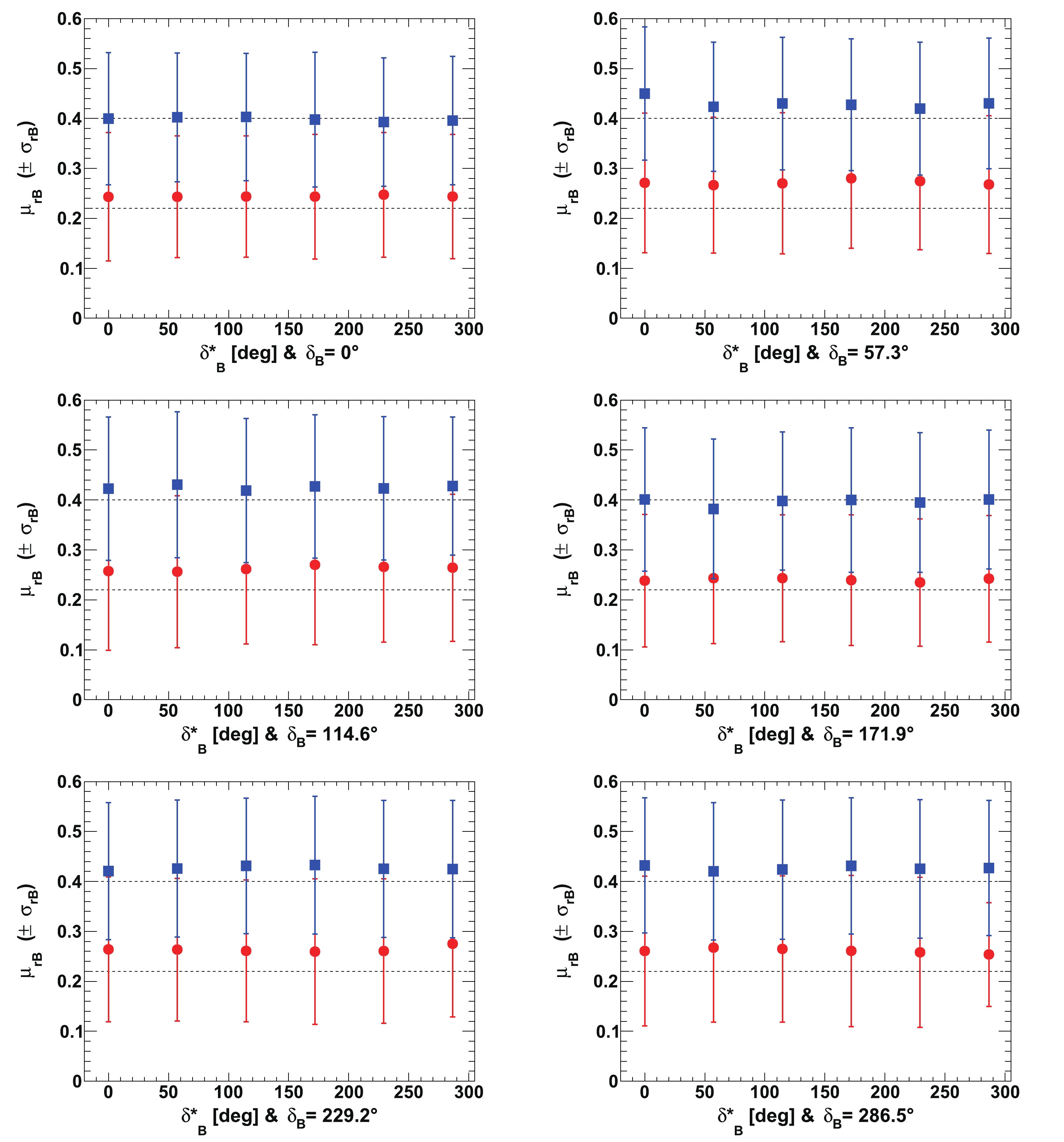
Figure A1. (color online) Fitted mean values of
${r_{B}}$ ($\mu_{{r_{B}}}$ ), for${r^{(*)}_{B}}=0.22$ (red circles) and 0.4 (blue squares) as a function of$\delta _B^{(*)}$ for initial true value of$\gamma$ of$65.66^\circ$ (1.146 rad). In each figure, the horizontal dashed black line indicates the initial${r_{B}}$ true value, and the displayed uncertainties are the fitted resolutions on${r_{B}}$ (i.e.$\sigma_{{r_{B}}}$ ).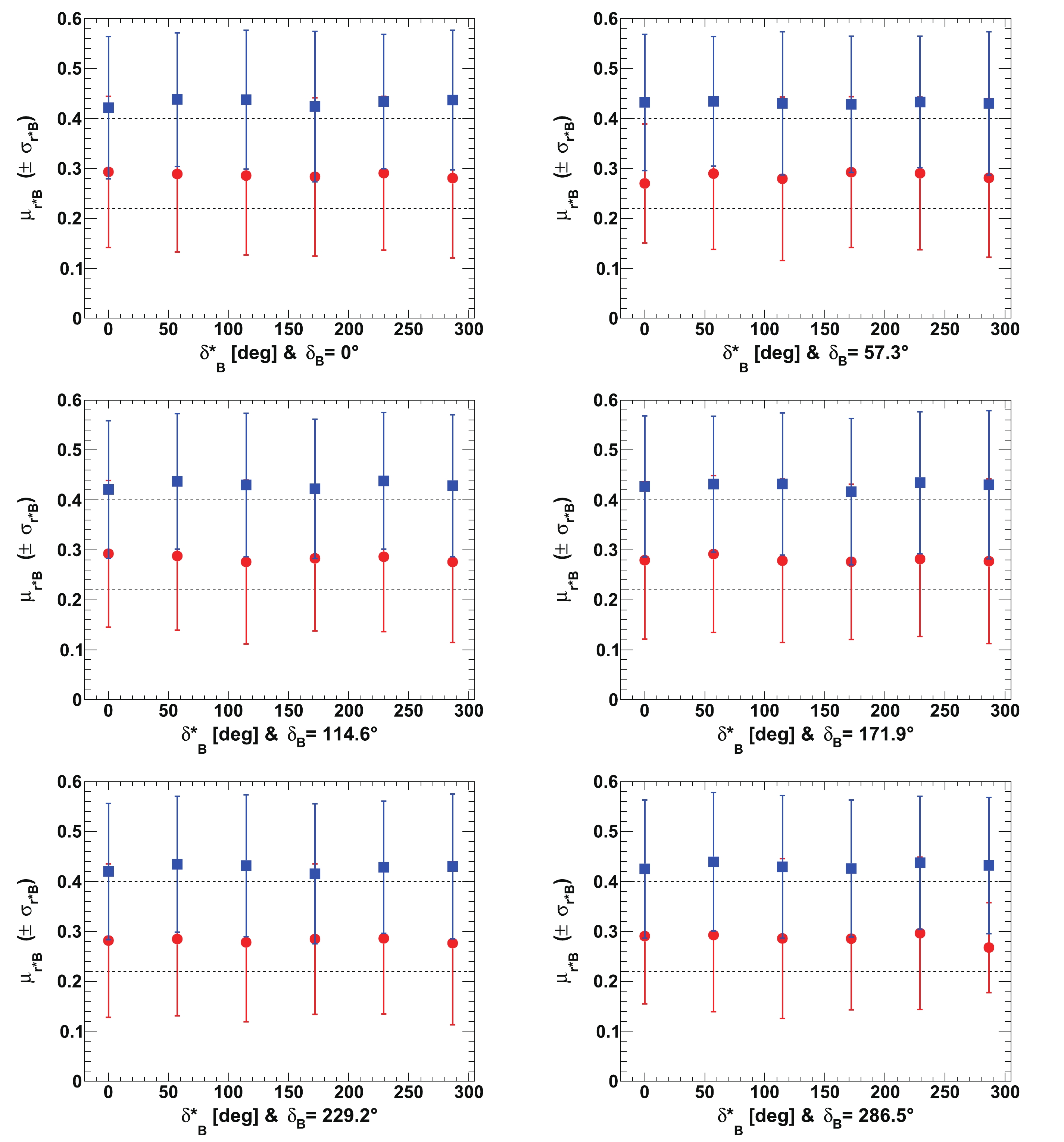
Figure A2. (color online) Fitted mean values of
${r^*_{B}}$ ($\mu_{{r^*_{B}}}$ ), for${r^{(*)}_{B}}=0.22$ (red circles) and 0.4 (blue squares) as a function of$\delta _B^{(*)}$ for initial true value of$\gamma$ of$65.66^\circ$ (1.146 rad). In each figure, the horizontal dashed black line indicates the initial${r^*_{B}}$ true value, and the displayed uncertainties are the fitted resolutions on${r^*_{B}}$ (i.e.$\sigma_{{r^*_{B}}}$ ).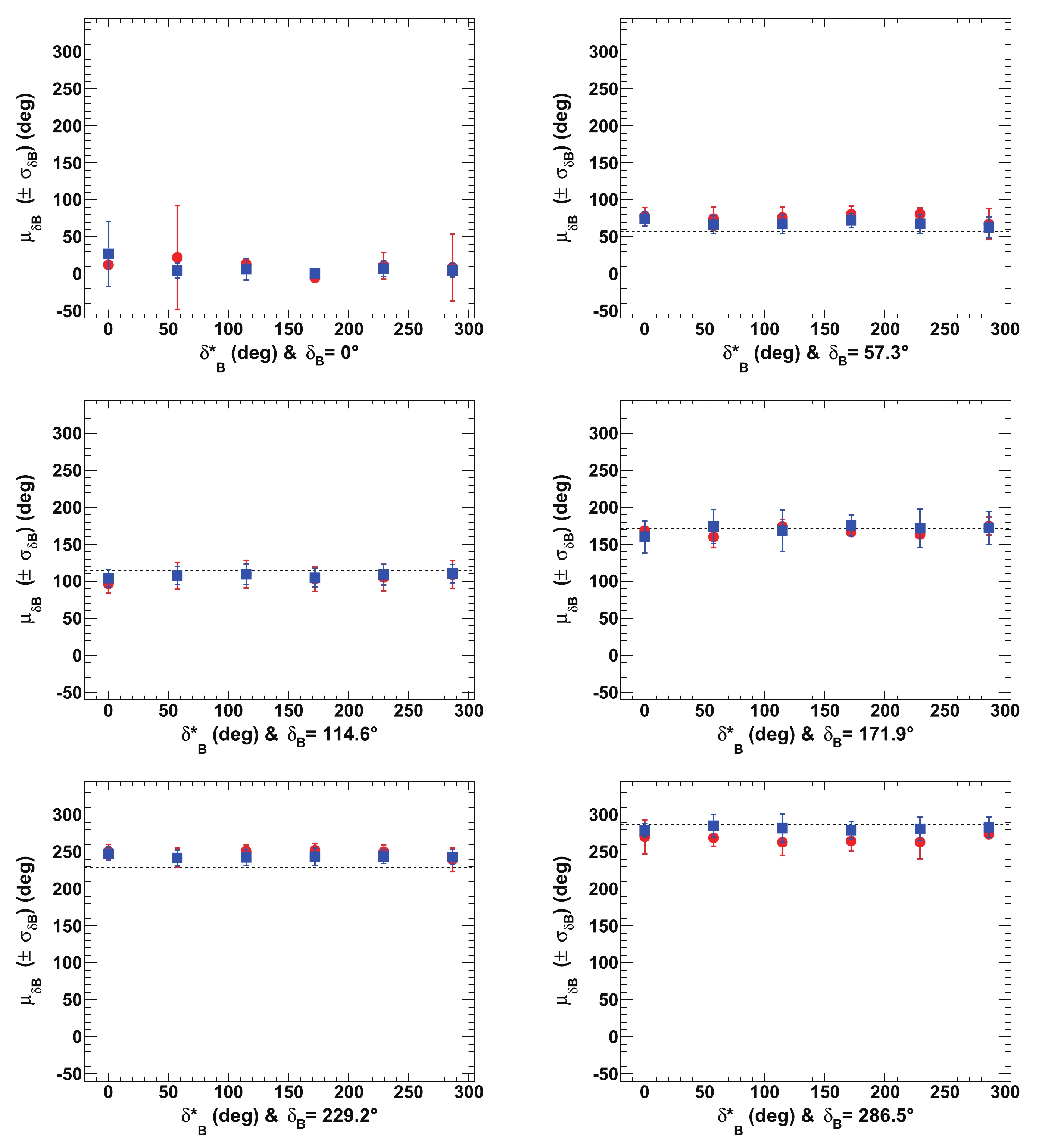
Figure A3. (color online) Fitted mean values of
${\delta_{B}}$ ($\mu_{{\delta_{B}}}$ ), for${r^{(*)}_{B}}=0.22$ (red circles) and 0.4 (blue squares) as a function of$\delta _B^{(*)}$ for initial true value of$\gamma$ of$65.66^\circ$ (1.146 rad). In each figure, the horizontal dashed black line indicates the initial${\delta_{B}}$ true value, and the displayed uncertainties are the fitted resolutions on${\delta_{B}}$ (i.e.$\sigma_{{\delta_{B}}}$ ).
Figure A4. (color online) Fitted mean values of
${\delta^*_{B}}$ ($\mu_{{\delta^*_{B}}}$ ), for${r^{(*)}_{B}}=0.22$ (red circles) and 0.4 (blue squares) as a function of$\delta _B^{(*)}$ for initial true value of$\gamma$ of$65.66^\circ$ (1.146 rad). In each figure, the dashed black line indicates the initial${\delta^*_{B}}$ true value, and the displayed uncertainties are the fitted resolutions on${\delta^*_{B}}$ (i.e.$\sigma_{{\delta^*_{B}}}$ ). -
Configurations in which
$ \gamma = 74^{\circ} $ (see Ref. [12]) have also been tested. The potential problem in this case is that, as the true value of$ \gamma $ is closer to the$ 90^\circ $ boundary, the unfolding of this parameter may become more difficult for many configurations of the nuisance parameters$ {{r^{(*)}_{B}}} $ and$ {{\delta^{(*)}_{B}}} $ . It is clear from Eq. (14) that the sensitivity to$ \gamma $ is null at$ 90^\circ $ . This is illustrated in Fig. B1 in Appendix B, which can be compared with Fig. 11. In this case, the initial tested configuration is$ \gamma = 74^{\circ} $ ,$ {{r^{(*)}_{B}}} = 0.4 $ and 0.22,$ {{\delta_{B}}} = 171.9^\circ $ (3 rad), and$ {{\delta^*_{B}}} = 114.6^\circ $ (2 rad). For these configurations,$ \mu_{\gamma} = \left( 73.7 \pm 0.3 \right)^\circ $ ($ \left( 74.2 \pm 0.7)^\circ\right) $ and$ \sigma_{\gamma} = \left( 7.7 \pm 0.3 \right)^\circ $ ($ \left( 14.7 \pm 0.6)^\circ \right) $ for$ {{r^{(*)}_{B}}} = 0.4 $ (0.22). There is limited degradation of the resolution compared to the corresponding configuration when the true value of$ \gamma $ is$ 65.66^\circ $ . The fit to$ \gamma $ for the pseudoexperiments corresponding to the configuration$ \gamma = 74^{\circ} $ ,$ {{r^{(*)}_{B}}} = 0.4 $ and 0.22,$ {{\delta_{B}}} = 57.3^\circ $ (1 rad), and$ {{\delta^*_{B}}} = 286.5^\circ $ (5 rad) is presented in Fig. B2 in Appendix B. For$ {{r^{(*)}_{B}}} = 0.22 $ , it can clearly be observed that the fitted$ \gamma $ value approaches the boundary limit of$ 90^\circ $ , and the corresponding resolution is approximately$ 18^\circ $ . Such behavior can be clearly understood from the 2-D distribution presented in Fig. 6. This is comparable to the case listed in Tables 5 and 6 when$ {{\delta^{(*)}_{B}}} = 286.5^\circ $ (near$ 3\pi/2 $ rad) and$ {{r^{(*)}_{B}}} = 0.22 $ .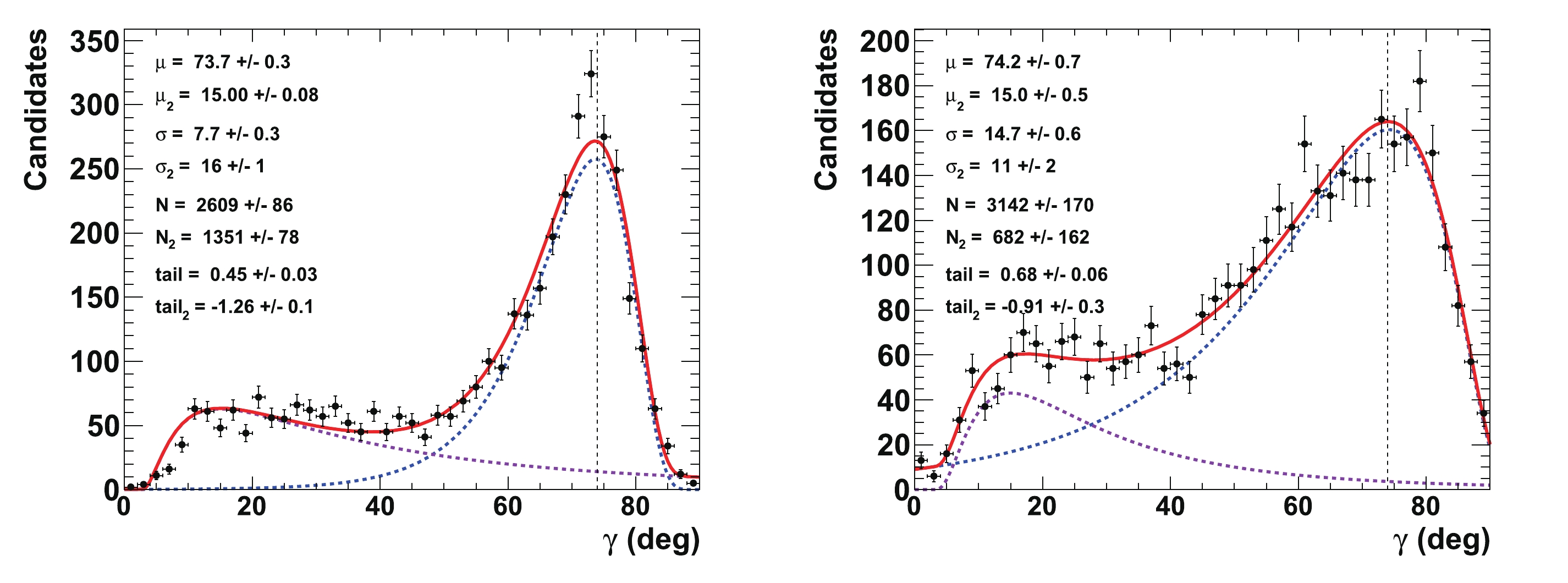
Figure B1. (color online) Fit to distributions of nuisance parameters
$\gamma$ obtained from 4000 pseudoexperiments. The initial configuration is$\gamma=74^{\circ}$ ,${r^{(*)}_{B}}=0.4$ (left) and 0.22 (right),${\delta_{B}}=171.9^\circ$ (3 rad), and${\delta^*_{B}}=114.6^\circ$ (2 rad). In the distributions, only the candidates with a value of$\gamma\ \in \ [0^\circ, \ 90^\circ]$ are considered. The purple dashed curve represents the tails generated by the correlations with the nuisance parameters${r^{(*)}_{B}}$ and$\delta _B^{(*)}$ , whereas the blue dashed curve indicates the core part of the distribution, and the plain red line is the sum of the two components of the fit.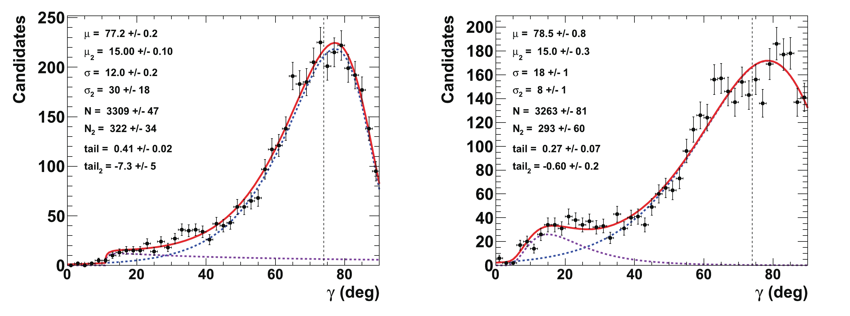
Figure B2. (color online) Fit to distributions of nuisance parameters
$\gamma$ obtained from 4000 pseudoexperiments. The initial configuration is$\gamma=74^{\circ}$ ,${r^{(*)}_{B}}=0.4$ (left) and 0.22 (right),${\delta_{B}}=57.9^\circ$ (1 rad), and${\delta^*_{B}}=286.5^\circ$ (5 rad). In the distributions, only the candidates with a value of$\gamma\ \in \ [0^\circ, \ 90^\circ]$ are considered. The purple dashed curve represents the tails generated by the correlations with the nuisance parameters${r^{(*)}_{B}}$ and$\delta _B^{(*)}$ , whereas the blue dashed curve indicates the core part of the distribution, and the plain red line is the sum of the two components of the fit. -
As listed in Table 2 the expected yields for the D-meson decays to
$ \pi\pi $ and$ K\pi{{\pi^{0}}} $ are somewhat lower than those for the other modes, down to a few tens of events. Again, these yields have been computed from LHCb studies on$ B^\pm \rightarrow \tilde{D}^{0}(\pi/K)^\pm $ , as reported in Refs. [28] and [29], and normalized to Ref. [22] with respect to the mode$ {{B^0_s}}\rightarrow \tilde{D}^{(*)0}(K\pi)\phi $ . Therefore, the selections are not necessarily against the signals$ {{B^0_s}}\rightarrow \tilde{D}^{(*)0}(\pi\pi)\phi $ and$ {{B^0_s}}\rightarrow \tilde{D}^{(*)0}(K\pi{{\pi^{0}}})\phi $ , and the expected yields may be underestimated, as well as all the sub-decays listed in Table 2. Furthermore, it should be noted that the mode$ \pi\pi $ is a$ CP $ -eigenstate, whereas the$ K\pi{{\pi^{0}}} $ 3-body decay also has a large coherence factor value$ R^{K\pi{{\pi^{0}}}}_D = (81\pm6) $ % [36]. Nevertheless, the effect of using the$ {{B^0_s}}\rightarrow \tilde{D}^{(*)0}(\pi\pi)\phi $ and$ {{B^0_s}}\rightarrow \tilde{D}^{(*)0}(K\pi{{\pi^{0}}})\phi $ decays or not has been studied and is reported here, and in Section VC, the effect of including the decays$ {{B^0_s}} \rightarrow {{\tilde{D}^{*0}}}\phi $ or not is also discussed for future more abundant datasets.According to Fig. C1 in Appendix C, there is a relative loss on the precision in the unfolded value of
$ \gamma $ of approximately$ 3 $ to$ 15 $ %, when the$ {{B^0_s}}\rightarrow \tilde{D}^{(*)0}(\pi\pi)\phi $ decays are not used. Figure C2 in Appendix C indicates that a relative loss in precision of approximately$ 3 $ to$ 22 $ % is observed when the$ {{B^0_s}}\rightarrow \tilde{D}^{(*)0}(K\pi{{\pi^{0}}})\phi $ decays are not used.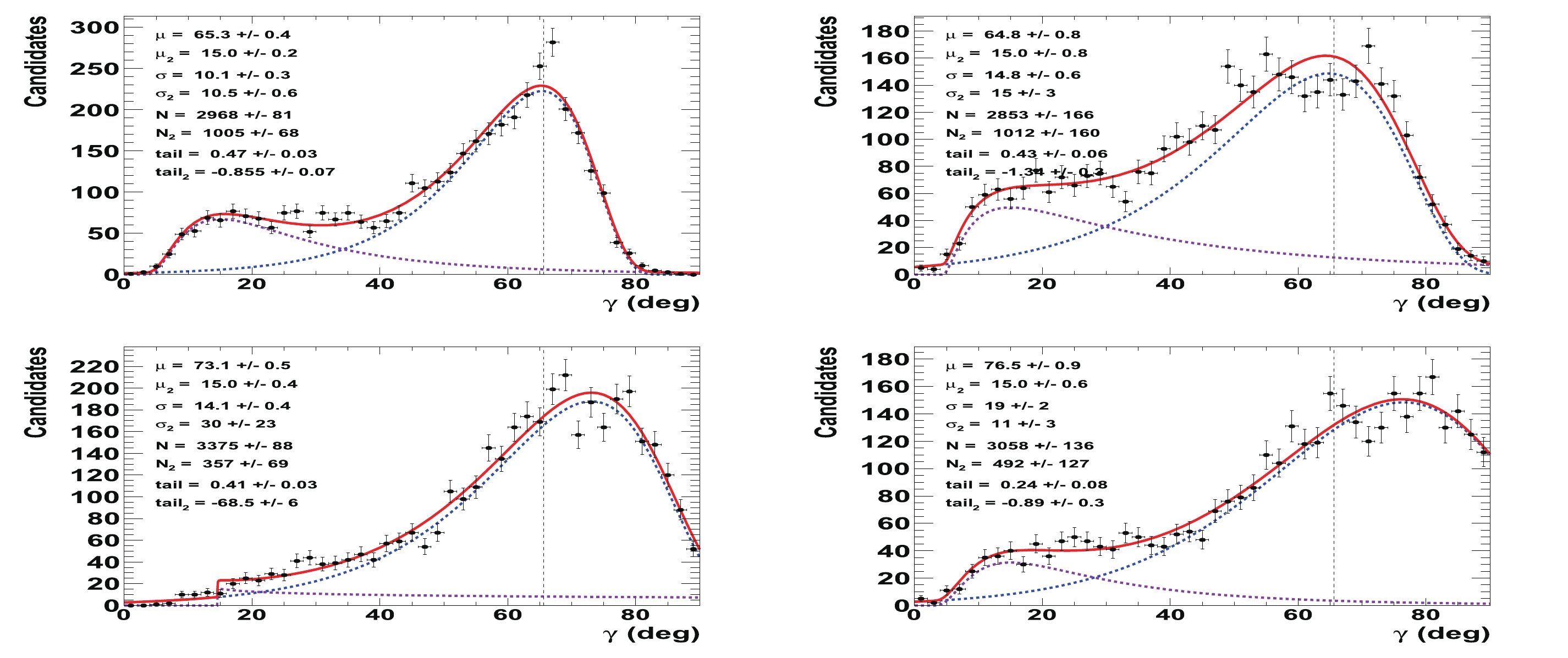
Figure C1. (color online) Fit to distributions of
$\gamma$ obtained from 4000 pseudoexperiments for Run 1 & 2 LHCb dataset. The initial configuration is$\gamma=65.66^{\circ}$ ,${r_{B}}=0.4$ (left) and 0.22 (right), and (top)${\delta_{B}}=171.9^\circ$ (3 rad) and${\delta^*_{B}}=114.6^\circ$ (2 rad) or (bottom)${\delta_{B}}=57.3^\circ$ (1 rad) and${\delta^*_{B}}=286.5^\circ$ (5 rad) (w/o${B^0_s} \rightarrow \tilde{D}^{(*)0}(\pi\pi)\phi$ ). The purple dashed curve represents the tails generated by the correlations with the nuisance parameters${r^{(*)}_{B}}$ and$\delta _B^{(*)}$ , whereas the blue dashed curve is the core part of the distribution, and the plain red line is the sum of the two components of the fit.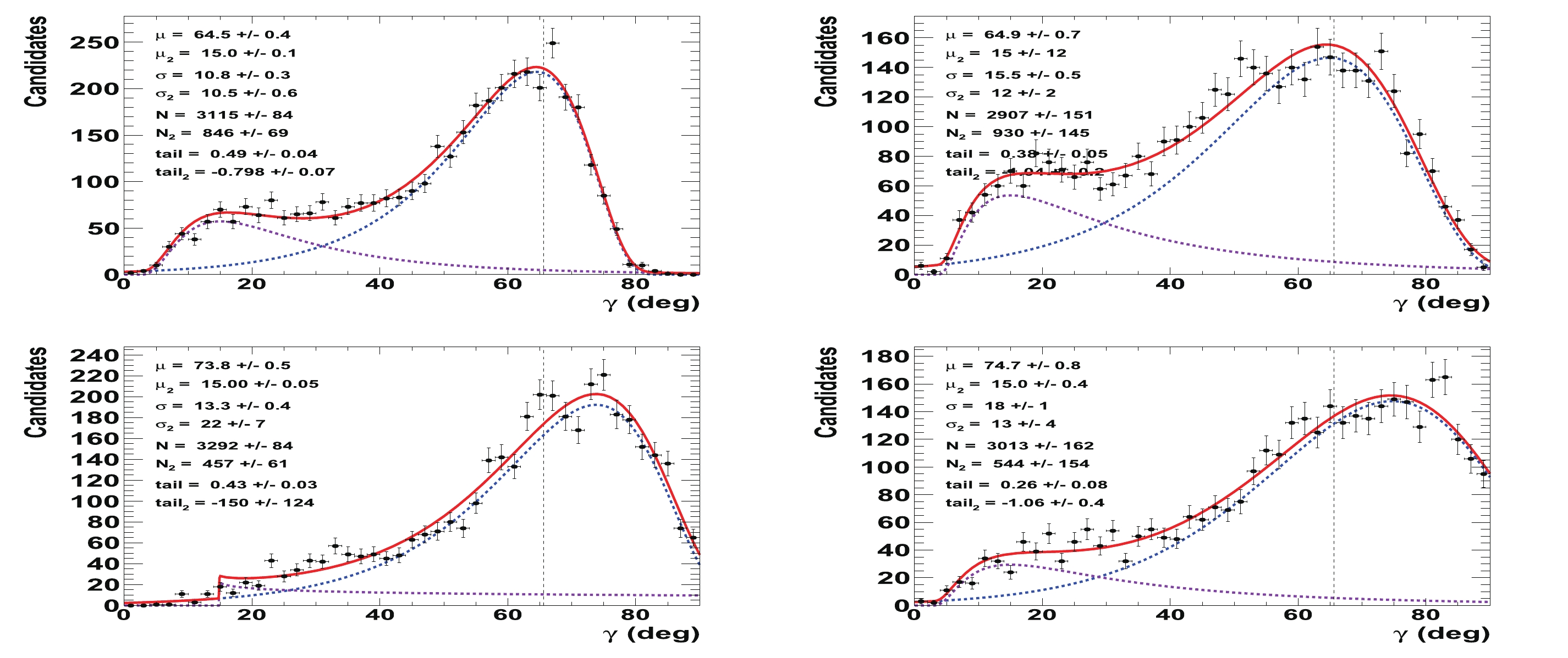
Figure C2. (color online) Fit to distributions of
$\gamma$ obtained from 4000 pseudoexperiments for Run 1 & 2 LHCb dataset. The initial configuration is$\gamma=65.66^{\circ}$ ,${r_{B}}=0.4$ (left) and 0.22 (right), and (top)${\delta_{B}}=171.9^\circ$ (3 rad) and${\delta^*_{B}}=114.6^\circ$ (2 rad) or (bottom)${\delta_{B}}=57.3^\circ$ (1 rad) and${\delta^*_{B}}=286.5^\circ$ (5 rad) (w/o${B^0_s} \rightarrow \tilde{D}^{(*)0}(K\pi{\pi^{0}})\phi$ ). The purple dashed curve represents the tails generated by the correlations with the nuisance parameters${r^{(*)}_{B}}$ and$\delta _B^{(*)}$ , whereas the blue dashed curve is the core part of the distribution, and the plain red line is the sum of the two components of the fit. -
The prospectives on the sensitivity to the CKM angle
$ \gamma $ with$ {{B^0_s}}\rightarrow \tilde{D}^{(*)0}\phi $ decays have also been studied for the foreseen LHCb integrated luminosities at the end of LHC Run 3 and for the possible full HL-LHC future LHCb program. According to Ref. [20], the LHCb trigger efficiency will be improved by a factor of 2 at the beginning of LHC Run 3. The full expected LHCb dataset of$ pp $ collisions at$ \sqrt{s} = 13 $ TeV corresponding to the sum of the Run 1, 2, and 3 LHCb dataset should be equal to 23 fb-1 by 2025, whereas it is expected to be 300 fb-1 by the second half of the 2030 decade. The final integrated LHCb luminosity accounts for an LHCb detector upgrade phase II. In the following, the projected event yields, as listed in Table 2, after 2025 and after 2038 have been scaled by a factor$F_{\rm later} = 6.3$ and$ 90 $ , respectively, and with uncertainties on observables of$1/\sqrt{F_{\rm later}}$ . -
For this prospective sensitivity study, we have made the conservative assumption that the precision on the strong parameters of the D-meson decays to
$ K\pi $ ,$ K3\pi $ , and$ K\pi{{\pi^{0}}} $ listed in Table 3 should be improved by a factor of 2 at the end of the LHCb program (see the BES-III experiment prospectives [54]). The procedure described for the LHCb Run 1 & 2 data in Section IV has been repeated. The values of the normalization factors$ C_{K\pi} $ ,$ C_{K\pi,D{{\pi^{0}}}} $ , and$ C_{K\pi,D\gamma} $ obtained for Run 1 & 2 (see Section III) have been scaled to their expected equivalent rate for Runs 1 to 3 and full HL-LHC LHCb datasets. The statistical uncertainties of the computed observables (see Secttion IVC) obtained for the Run 1 & 2 LHCb data have been scaled by the square root of a factor two times (trigger improvement) the relative increase in the anticipated collected$ {{B^0_s}} $ -meson yield: 2.2 (8.8) for the Run 1 to 3 (full HL-LHC) LHCb dataset. Thereafter, for the Run 1 & 2 sensitivity studies, the same$ 2 \times 6 \times 6 $ configurations of the$ {{r^{(*)}_{B}}} $ , and$ {{\delta^{(*)}_{B}}} $ nuisance parameters have been tested ($ {{r^{(*)}_{B}}} = 0.22 $ or 0.4 and$ {{\delta^{(*)}_{B}}} = 0 $ , 1, 2, 3, 4, 5 rad, and$ \gamma = 65.66^{\circ} $ (1.146 rad)).The 2-D p-value distribution profiles of the nuisance parameters
$ {{r^{(*)}_{B}}} $ and$ {{\delta^{(*)}_{B}}} $ as a function of$ \gamma $ are presented in Figs. 15 and 16 for the expected Run$ 1-3 $ LHCb dataset, and in Figs. 17 and 18 for the full HL-LHC LHCb dataset. For the purpose of these illustrations, the initial configuration of true values is$ \gamma = 65.66^\circ $ (1.146 rad),$ {{\delta_{B}}} = 171.9^\circ $ (3.0 rad), and$ {{\delta^*_{B}}} = 114.6^\circ $ (2.0 rad), as well as$ {{r^{(*)}_{B}}} = 0.4 $ (0.22). Therefore, the distributions can be directly compared to those depicted in Figs. 7 and 8. The surface of the excluded regions at a 95.4% CL in$ {{r^{(*)}_{B}}} \ vs. \ \gamma $ and$ {{\delta^{(*)}_{B}}} \ vs. \ \gamma $ clearly increases with the additional data, but even in the semi-asymptotic regime, for the full expected HL-LHC LHCb dataset, one can clearly observe possible strong correlations between$ \gamma $ and the nuisance parameters$ {{r^{(*)}_{B}}} $ and$ {{\delta^{(*)}_{B}}} $ . This is also visible in Figs. D1 and D2 in Appendix D, which are the equivalent version for the full expected HL-LHC LHCb dataset of the Run 1 & 2 LHCb dataset presented in Figs. 5 and 6 for the configurations$ \gamma = 65.66^\circ $ (1.146 rad),$ {{\delta_{B}}} = 57.3^\circ $ (1.0 rad), and$ {{\delta^*_{B}}} = 286.5^\circ $ (5.0 rad), as well as$ {{r^{(*)}_{B}}} = 0.4 $ (0.22).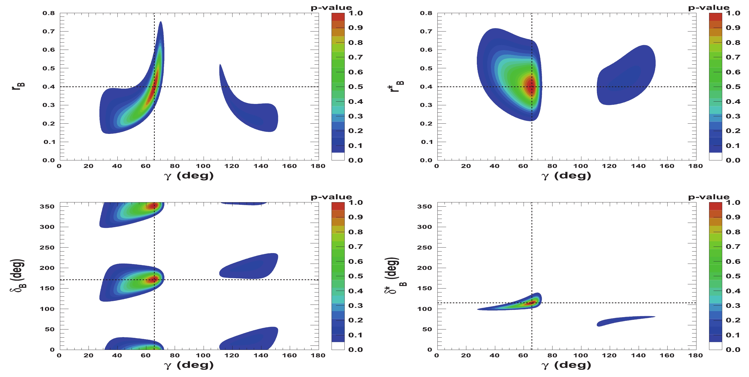
Figure 15. (color online) 2-D p-value profiles of nuisance parameters
${r^{(*)}_{B}}$ and$\delta _B^{(*)}$ (Runs$1-3$ ) as a function of$\gamma$ . In each figure, the dashed black lines indicate the initial true values$\gamma=65.66^\circ$ (1.146 rad),${\delta_{B}}=171.9^\circ$ (3.0 rad), and${\delta^*_{B}}=114.6^\circ$ (2.0 rad), as well as${r^{(*)}_{B}}=0.4$ .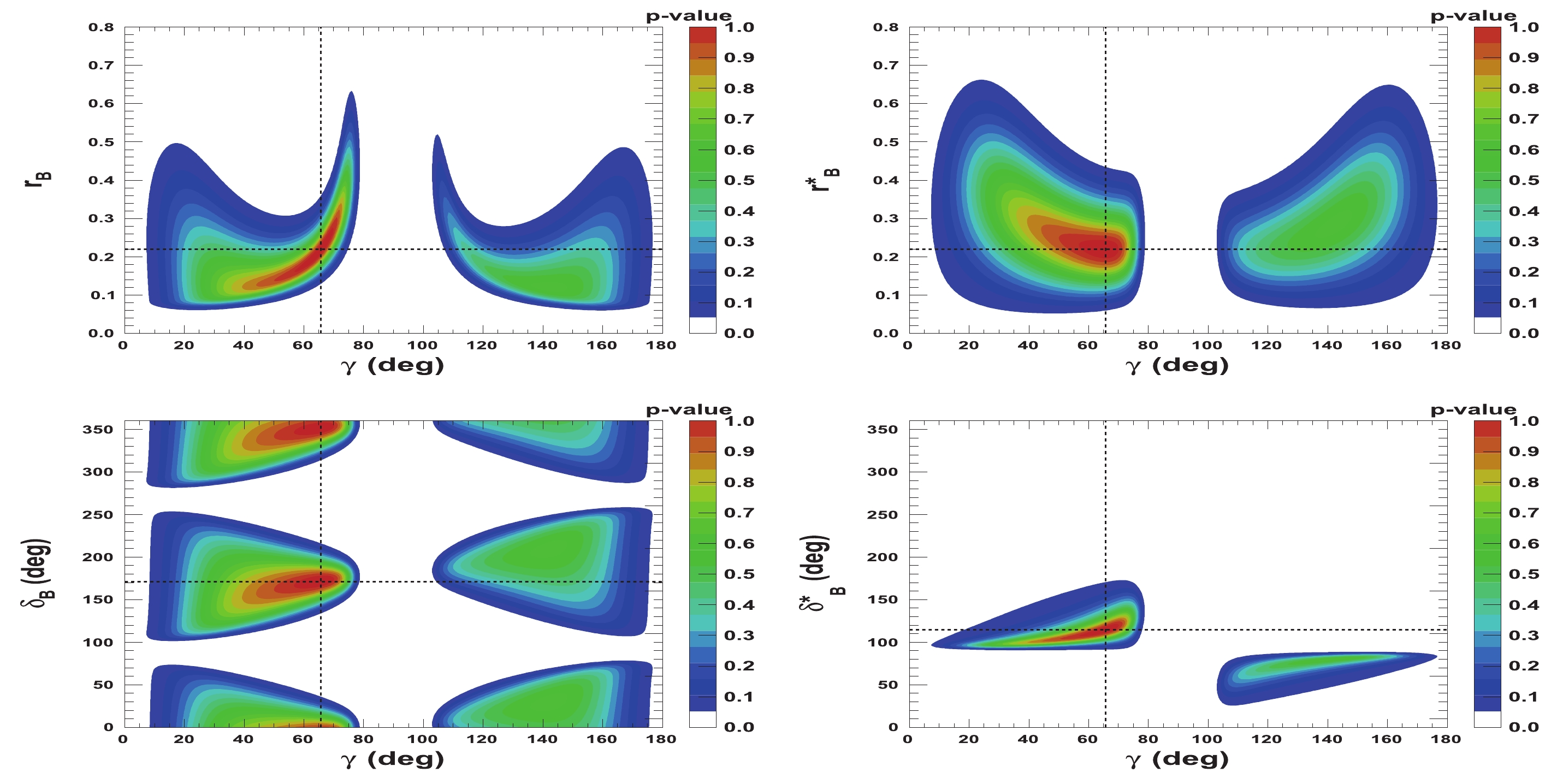
Figure 16. (color online) 2-D p-value profiles of nuisance parameters
${r^{(*)}_{B}}$ and$\delta _B^{(*)}$ for Run$1-3$ LHCb dataset as a function of$\gamma$ . In each figure, the dashed black lines indicate the initial true values$\gamma=65.66^\circ$ (1.146 rad),${\delta_{B}}=171.9^\circ$ (3.0 rad), and${\delta^*_{B}}=114.6^\circ$ (2.0 rad), as well as${r^{(*)}_{B}}=0.22$ .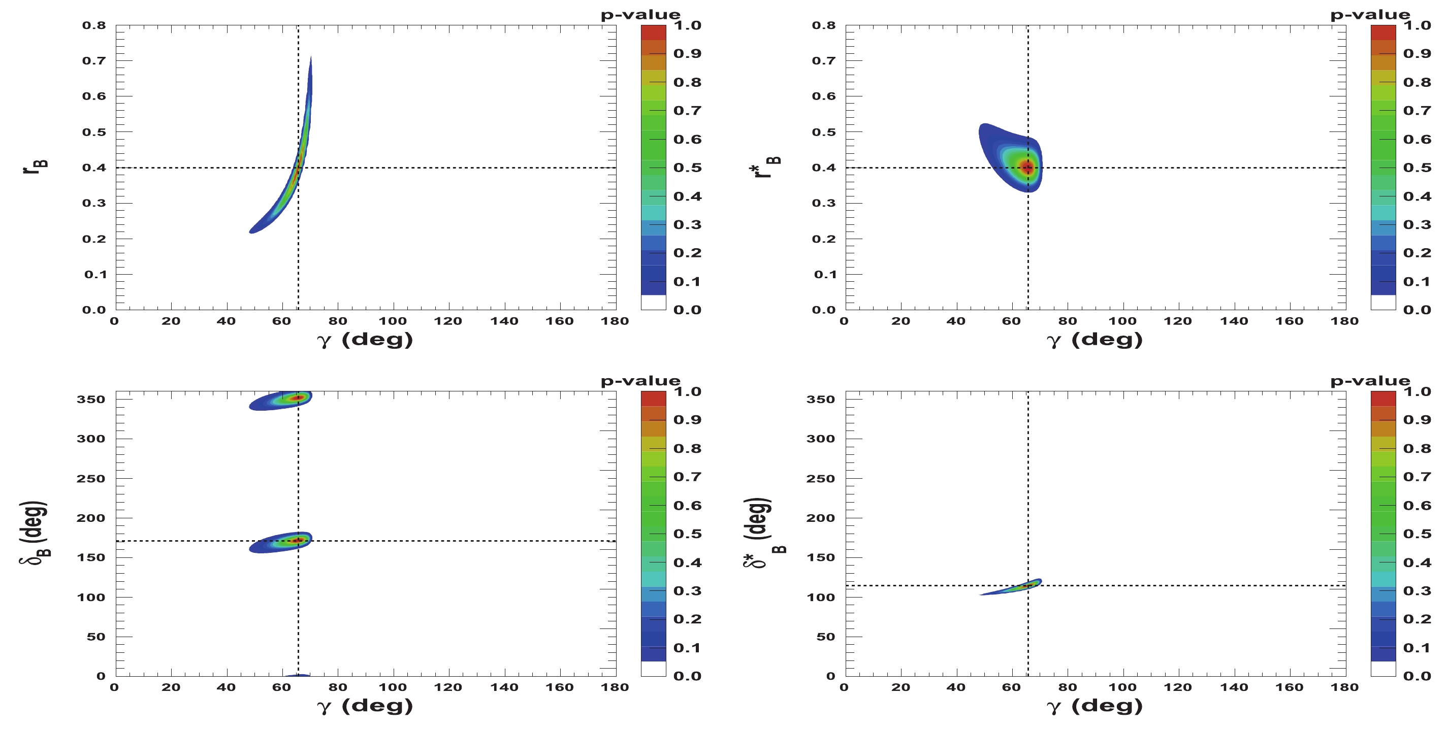
Figure 17. (color online) 2-D p-value profiles of nuisance parameters
${r^{(*)}_{B}}$ and$\delta _B^{(*)}$ for full HL-LHC LHCb dataset as a function of$\gamma$ . In each figure, the dashed black lines indicate the initial true values$\gamma=65.66^\circ$ (1.146 rad),${\delta_{B}}=171.9^\circ$ (3.0 rad), and${\delta^*_{B}}=114.6^\circ$ (2.0 rad), as well as${r^{(*)}_{B}}=0.4$ .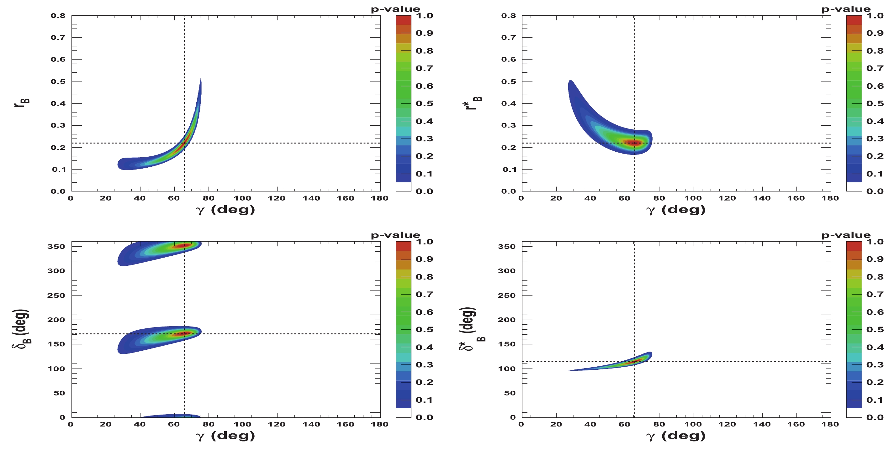
Figure 18. (color online) 2-D p-value profiles of nuisance parameters
${r^{(*)}_{B}}$ and$\delta _B^{(*)}$ for full HL-LHC LHCb dataset as a function of$\gamma$ . In each figure, the dashed black lines indicate the initial true values$\gamma=65.66^\circ$ (1.146 rad),${\delta_{B}}=171.9^\circ$ (3.0 rad), and${\delta^*_{B}}=114.6^\circ$ (2.0 rad), as well as${r^{(*)}_{B}}=0.22$ .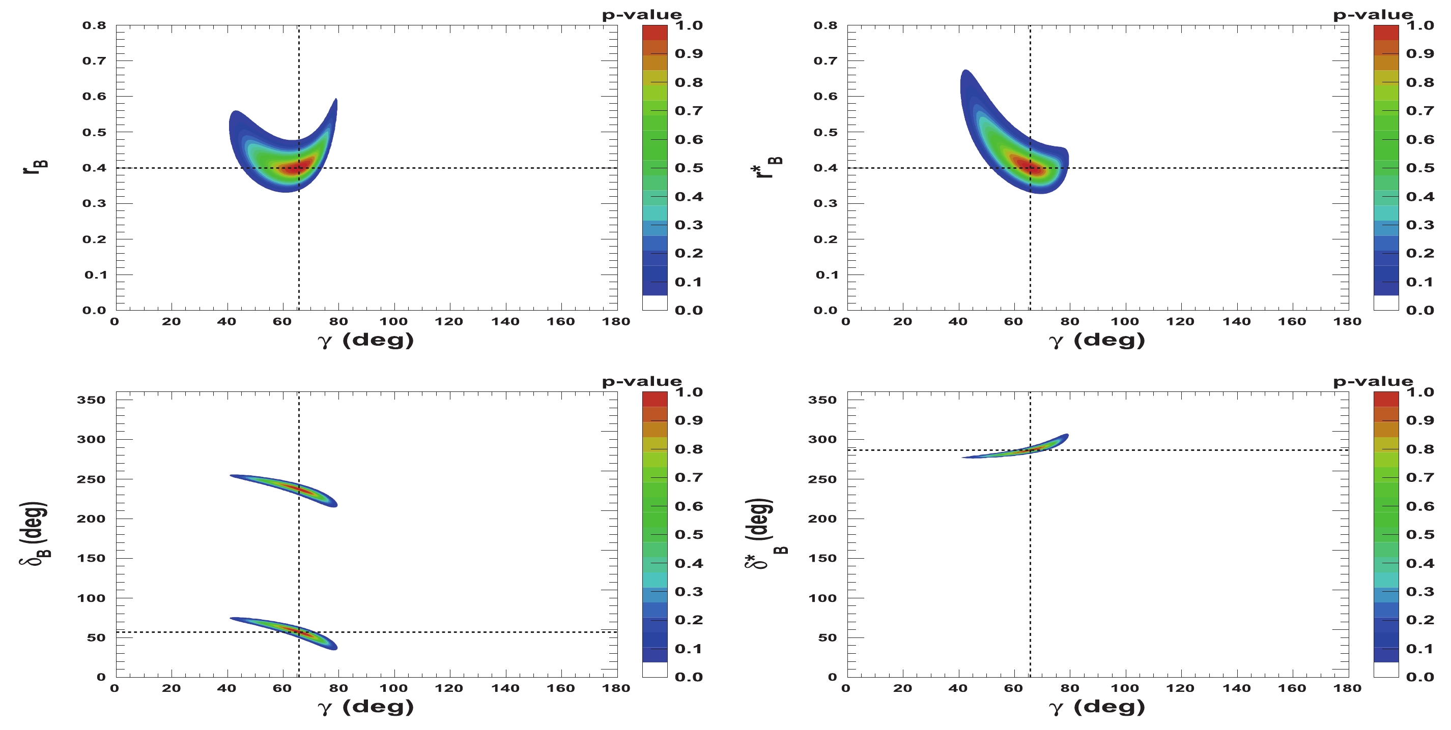
Figure D1. (color online) 2-D p-value profiles of nuisance parameters
${r^{(*)}_{B}}$ and$\delta _B^{(*)}$ for full HL-LHC LHCb dataset as a function of$\gamma$ . In each figure, the dashed black lines indicate the initial${r^{(*)}_{B}}$ and$\delta _B^{(*)}$ ($\gamma$ ) true values:$\gamma=65.66^\circ$ (1.146 rad),${\delta_{B}}=57.3^\circ$ (1.0 rad), and${\delta^*_{B}}=286.5^\circ$ (5.0 rad), as well as${r^{(*)}_{B}}=0.4$ .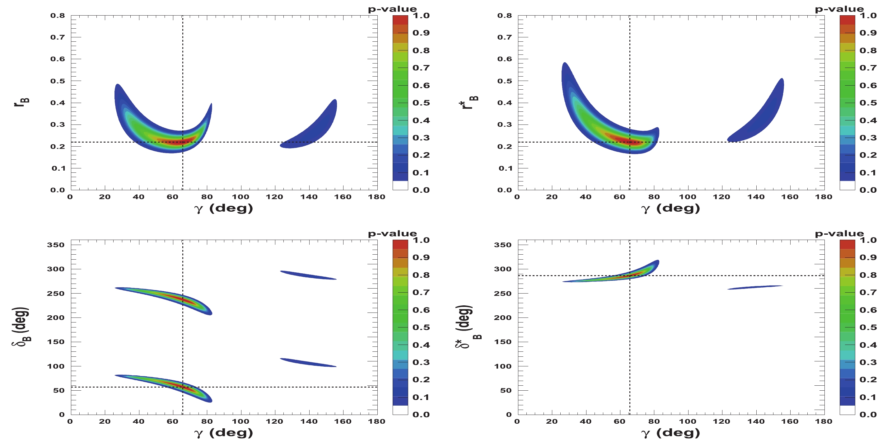
Figure D2. (color online) 2-D p-value profiles of nuisance parameters
${r^{(*)}_{B}}$ and$\delta _B^{(*)}$ for full HL-LHC LHCb dataset as a function of$\gamma$ . In each figure, the dashed black lines indicate the initial true values$\gamma=65.66^\circ$ (1.146 rad),${\delta_{B}}=57.3^\circ$ (1.0 rad), and${\delta^*_{B}}=286.5^\circ$ (5.0 rad), as well as${r^{(*)}_{B}}=0.22$ .For the configuration
$ \gamma = 65.66^\circ $ (1.146 rad),$ {{\delta_{B}}} = $ $171.9^\circ $ (3.0 rad), and$ {{\delta^*_{B}}} = 114.6^\circ $ (2.0 rad), as well as$ {{r^{(*)}_{B}}} = 0.4 $ (0.22), Fig. 19 presents the fitted$ \gamma $ distribution obtained for 4000 pseudoexperiments for the expected Run$ 1-3 $ LHCb dataset. The fitted values are$ \mu_{\gamma} = \left( 67.7 \pm 0.1 \right)^\circ $ $ \left( (73.5 \pm 0.2)^\circ \right) $ and$ \sigma_{\gamma} = \left( 3.5 \pm 0.1 \right)^\circ $ $ \left( (5.5 \pm 0.2)^\circ \right) $ for$ {{r^{(*)}_{B}}} = 0.4 $ (0.22). The fitted values presented in Fig. 21 are$ \mu_{\gamma} = ( 68.1 \pm $ $0.1 )^\circ $ $ \left( (71.1 \pm 0.1)^\circ\right) $ and$ \sigma_{\gamma} = \left( 2.5 \pm 0.1 \right)^\circ $ $ \left( (5.3 \pm 0.1)^\circ \right) $ for$ {{r^{(*)}_{B}}} = 0.4 $ (0.22), respectively, for the expected full HL-LHC LHCb dataset. The fitted values are slightly shifted up with respect to the initial$ \gamma $ true value but are compatible within one standard deviation. When comparing with the numbers listed in Table 6, it can be observed that the resolution improves as$ 8.8/3.5 = 2.5 $ ($ 14.4/5.5 = 2.6) $ for$ {{r^{(*)}_{B}}} = 0.4 $ (0.22) when moving from the Run 1 & 2 to the expected Run$ 1-3 $ LHCb datasets, whereas a factor of 2.2 is expected. However, when moving from the expected Run$ 1-3 $ to the full expected HL-LHC LHCb datasets, the improvement is only$ 3.5/2.5 = 1.4 $ ($ 5.5/5.3 = 1.040) $ for$ {{r^{(*)}_{B}}} = 0.4 $ (0.22), whereas one may naively expect an improvement$ 8.8/2.2 = 4.0 $ . This is certainly partially owing to the strong correlations between the nuisance parameters$ {{r^{(*)}_{B}}} $ and$ {{\delta^{(*)}_{B}}} $ . A more sophisticated simultaneous global fit to the nuisance parameters$ {{r^{(*)}_{B}}} $ and$ {{\delta^{(*)}_{B}}} $ , and$ \gamma $ may be useful.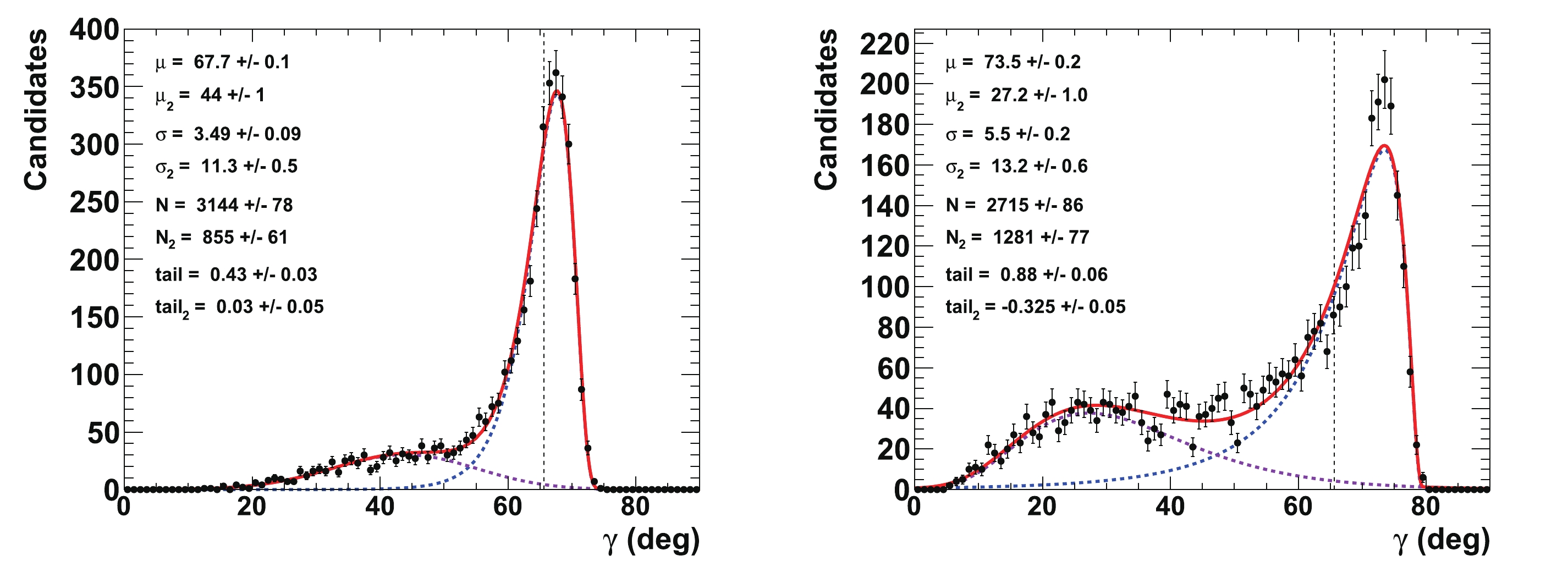
Figure 19. (color online) Fit to distributions of
$\gamma$ obtained from 4000 pseudoexperiments for expected Run$1-3$ LHCb dataset. The initial configuration is$\gamma=65.66^{\circ}$ ,${r^{(*)}_{B}}=0.4$ (left) and 0.22 (right),${\delta_{B}}=171.9^\circ$ (3 rad), and${\delta^*_{B}}=114.6^\circ$ (2 rad). The purple dashed curve represents the tails generated by the correlations with the nuisance parameters${r^{(*)}_{B}}$ and$\delta _B^{(*)}$ , whereas the blue dashed curve indicates the core part of the distribution, and the plain red line is the sum of the two components of the fit.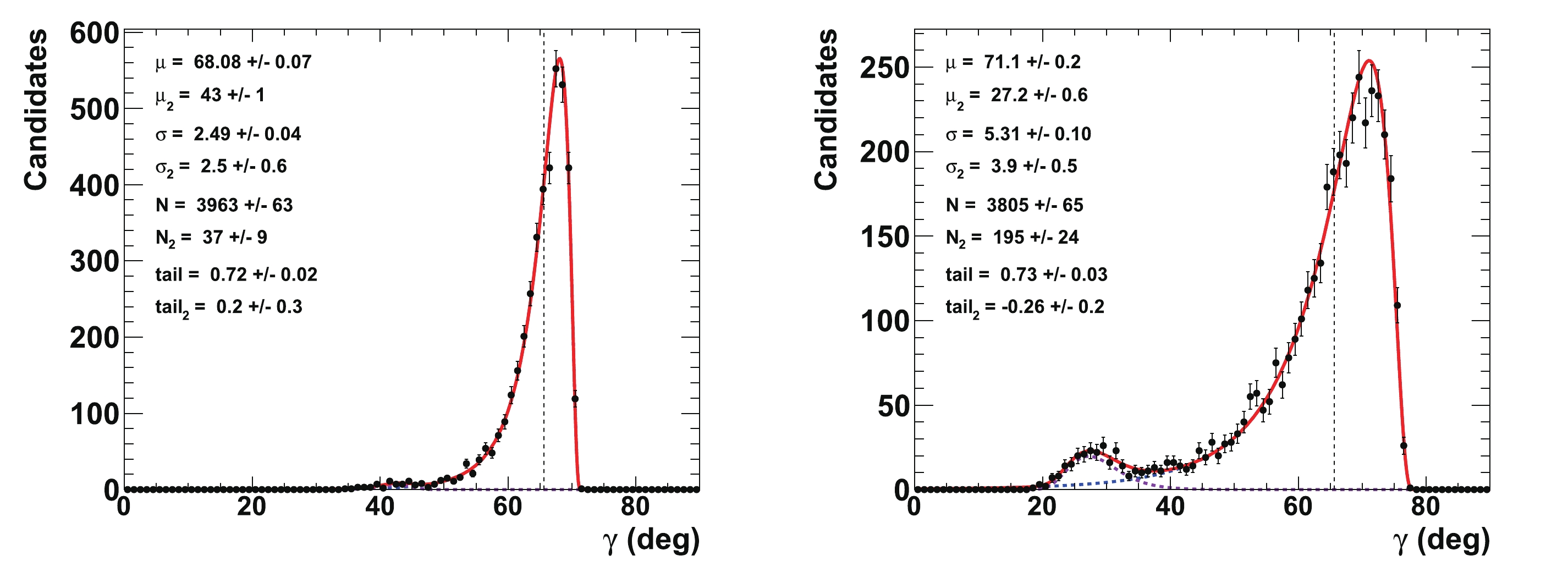
Figure 21. (color online) Fit to distributions of
$\gamma$ obtained from 4000 pseudoexperiments for expected full HL-LHC LHCb dataset. The initial configuration is$\gamma=65.66^{\circ}$ ,${r^{(*)}_{B}}=0.4$ (left) and 0.22 (right),${\delta_{B}}=171.9^\circ$ (3 rad), and${\delta^*_{B}}=114.6^\circ$ (2 rad). The purple dashed curve represents the tails generated by the correlations with the nuisance parameters${r^{(*)}_{B}}$ and$\delta _B^{(*)}$ , whereas the blue dashed curve is the core part of the distribution, and the plain red line is the sum of the two components of the fit.It must also be remembered that
$ {\mathtt{TMath::Prob}}$ still exhibits some under-coverage, namely 79$ (91) $ % and 94$ (89) $ % for$ {{r^{(*)}_{B}}} = 0.4 $ (0.22), with respect to the full frequentist treatment on the Monte-Carlo simulation basis [50], as presented in Fig. 23, with the Run$ 1-3 $ and full expected HL-LHC LHCb datasets, respectively. The relative scale factors$ F_{K3\pi} $ ,$ F_{K\pi{{\pi^{0}}}} $ ,$ F_{KK} $ , and$ F_{\pi\pi} $ used in this study already have a precision above 2%. The precision on the normalization factors$ C_{K\pi} $ ,$ C_{K\pi,D{{\pi^{0}}}} $ , and$ C_{K\pi,D\gamma} $ may also benefit from another improved precision of the branching fraction of the decay modes$ {{B^0_s}}\rightarrow {\kern 0.2em\overline{\kern -0.2em D}{}}^{(*)0}\phi $ and of the longitudinal polarization fraction in the mode$ {{B^0_s}}\rightarrow {\kern 0.2em\overline{\kern -0.2em D}{}}^{*0}\phi $ . However, the normalization factors are the same for all sets of Eqs. (14)-(34) for$ {{B^0_s}} \rightarrow {{\tilde{D}^0}} \phi $ or$ {{\tilde{D}^{*0}}} ({{\pi^{0}}}, \ \gamma)\phi $ , and their improved precision should be a second order effect. All of the above listed improvements are expected to occur to benefit from the total expected HL-LHC LHCb dataset fully.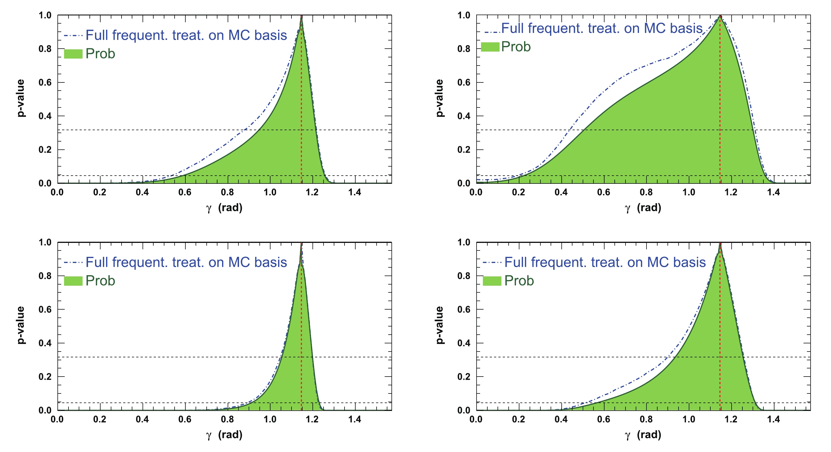
Figure 23. (color online) Profiles of p-value distributions of global
$\chi^2$ fit to$\gamma$ for set of true initial parameters$\gamma=1.146$ rad,${r^{(*)}_{B}}=0.4$ (left)$0.22$ (right),${\delta_{B}}=3.0$ rad, and${\delta^*_{B}}=2.0$ rad. The assumed integrated luminosity is that of the LHCb data expected to be collected after LHC Run 3 (top) and after the full HL-LHC (bottom) period. The corresponding distribution obtained from the full frequentist treatment on the Monte Carlo simulation basis [50] is superimposed on the profile obtained with$ {\mathtt{TMath::Prob}}$ . In each figure, the vertical dashed red line indicates the initial$\gamma$ true value, and the two horizontal dashed black lines refer to 68.3 and 95.4% CLs.The expected resolutions on
$ \gamma $ for the other usual configuration ($ {{\delta^{(*)}_{B}}} = 0 $ , 1, 2, 3, 4, 5 rad, and$ \gamma = 65.66^{\circ} $ (1.146 rad)) are presented in Fig. 20 for$ {{r^{(*)}_{B}}} = 0.4 $ and in Fig. 22 for$ {{r^{(*)}_{B}}} = 0.22 $ , for the Run 1 & 2, Run$ 1-3 $ , and full HL-LHC LHCb datasets. For$ {{r^{(*)}_{B}}} = 0.4 $ , the resolution mainly ranges from$ 3.4^\circ $ to$ 7.8^\circ $ for Run$ 1-3 $ and from$ 2.2^\circ $ to$ 7.1^\circ $ , or better, for the full HL-LHC dataset. For$ {{r^{(*)}_{B}}} = 0.22 $ , the resolution ranges from$ 5.5^\circ $ to$ 8.2^\circ $ for Run$ 1-3 $ and from$ 3.3^\circ $ to$ 7.8^\circ $ , or better, for the full HL-LHC dataset.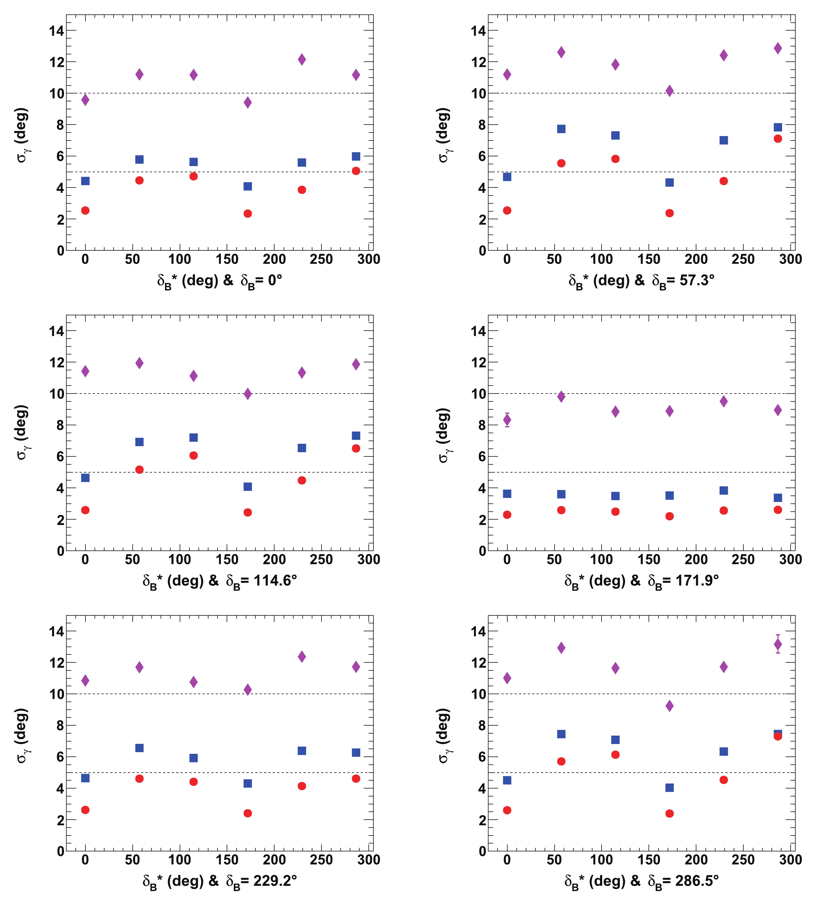
Figure 20. (color online) Fitted mean values of
$\gamma$ ($\sigma_{\gamma}$ ) for Run 1 & 2 (pink lozenges), Run$1-3$ (blue squares), and full HL-LHC (red circles) LHCb dataset as a function of$\delta _B^{(*)}$ , for${r^{(*)}_{B}}=0.4$ and initial true value of$65.66^\circ$ (1.146 rad). In each figure, the horizontal dashed black lines are guides for the eye at$\sigma_{\gamma}=5^\circ$ and$10^\circ$ .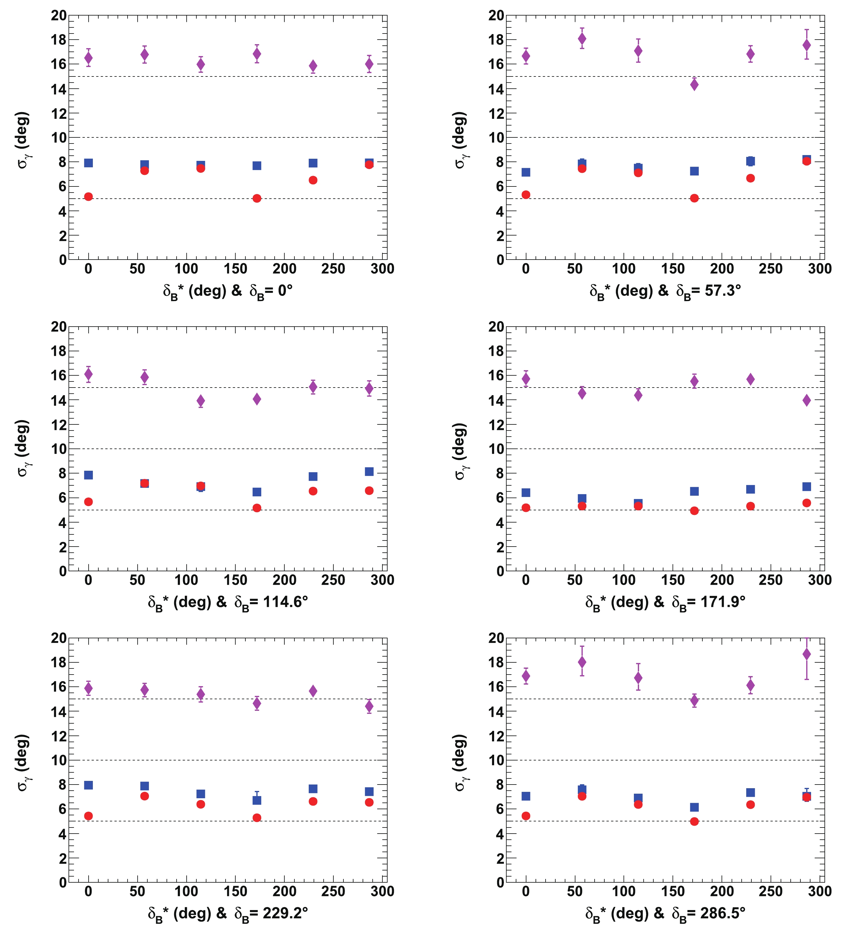
Figure 22. (color online) Fitted resolutions of
$\gamma$ ($\sigma_{\gamma}$ ) for Run 1 & 2 (pink lozenges), Run$1-3$ (blue squares), and full HL-LHC (red circles) LHCb dataset as a function of$\delta _B^{(*)}$ , for${r^{(*)}_{B}}=0.22$ and initial true value of$65.66^\circ$ (1.146 rad). In each figure, the horizontal dashed black lines are guides for the eye at$\sigma_{\gamma}=5^\circ, \ 10^\circ,$ and$15^\circ$ .Another expected improvement could arise from a time-dependent CP Dalitz plane analysis of the decay
$ {{B^0_s}} \rightarrow \tilde{D}^{(*)0}_{CP} {{K^{+}}} {{K^{-}}} $ , as anticipated in Ref. [55]. With the ultimate HL-LHC LHCb dataset, it should be possible to perform such an analysis, thus including the$ {{B^0_s}}\rightarrow \tilde{D}^{(*)0}\phi $ decay, to extract the CKM angle$ \gamma $ , as proposed a few years ago in [56].For completeness, an alternate definition of the resolution as half of the 68.3% CL frequentist intervals of the 1-D p-value profiles of a 68.3% CL is provided in Appendix E in Figs. E1 and E2. A better scaling of the performances is observed with the size of the datasets, whereas relatively worse resolutions are obtained with respect to those displayed in Figs. 20 and 22. However, the effects of the nuisance parameters
$ {{r^{(*)}_{B}}} $ and$ {{\delta^{(*)}_{B}}} $ are treated in a simplified manner compared to the full treatment by the generated pseudoexperiments.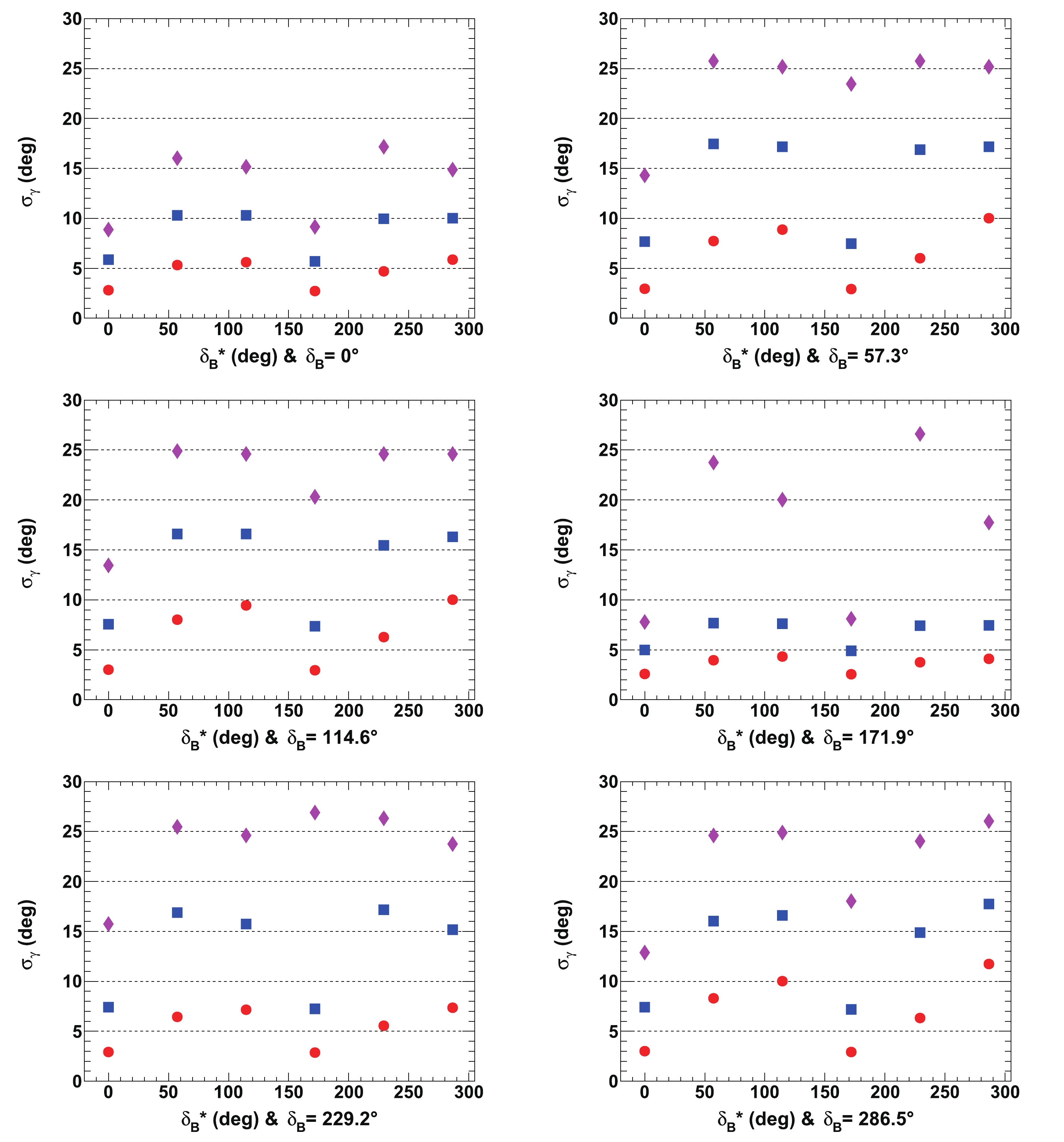
Figure E1. (color online) Half of 68.3% CL intervals of 1-D p-value profiles of
$\gamma$ for Run 1 & 2 (pink lozenges), Run$1-3$ (blue squares), and full HL-LHC (red circles) LHCb dataset as a function of$\delta _B^{(*)}$ , for${r^{(*)}_{B}}=0.4$ and initial true value of$65.66^\circ$ . In each figure, the horizontal dashed black lines are guides for the eye.
Figure E2. (color online) Half of 68.3% CL intervals of 1-D p-value profiles of
$\gamma$ for Run 1 & 2 (pink lozenges), Run$1-3$ (blue squares), and full HL-LHC (red circles) LHCb dataset as a function of$\delta _B^{(*)}$ , for${r^{(*)}_{B}}=0.22$ and initial true value of$65.66^\circ$ . In each figure, the horizontal dashed black lines are guides for the eye. -
Most of the strong parameters of the D-meson decays to
$ K\pi $ ,$ K3\pi $ , and$ K\pi{{\pi^{0}}} $ are external parameters and are obtained from beauty- or charm-factories, such as BaBar, Belle, CLEO-c, and LHCb [27]. Improvements in their determination are expected soon from the updated BES-III experiment [50] or later, from future super$ \tau $ -charm factories [57-59]. Several scenarios have been tested to verify the effects of these improvements to the$ \gamma $ sensitivity. With the set of parameters$ \gamma = 1.146 $ rad ($ 65.66^\circ $ ),$ {{r^{(*)}_{B}}} = 0.4 $ , and$ {{\delta_{B}}} = 3.0 $ rad, as well as$ {{\delta^*_{B}}} = 2.0 $ , the uncertainties of the current measurements of the D-meson parameters listed in Table 3 have been scaled down, and their effects on the fitted$ \gamma $ values from pseudoexperiments are listed in Table 7. As the uncertainties of the external parameters are not yet dominant (Run 1 & 2 data), a study has also been performed for the expected full HL-LHC dataset. However, with substantially more data, future improvements in the measurements of the strong parameters from the D-meson decays do not appear to influence the sensitivity to the CKM angle$ \gamma $ significantly.Uncertainties of D-meson params. Now $ \times 1/2 $ 

$ \times 1/5 $ 

$ \times 1/10 $ 

Run 1 & 2 ( $ {{r^{(*)}_{B}}}=0.4 $ )

$ 8.8 \pm 0.2 $ 

$ 8.1 \pm 0.3 $ 

$ 8.0\pm 0.3 $ 

$ 7.8\pm0.2 $ 

Run 1 & 2 ( $ {{r^{(*)}_{B}}}=0.22 $ )

$ 12.9 \pm 0.3 $ 

$ 13.2\pm 0.5 $ 

$ 13.1\pm0.5 $ 

$ 12.8\pm0.9 $ 

Full HL-LHC ( $ {{r^{(*)}_{B}}}=0.4 $ )

$ 2.6\pm0.1 $ 

$ 2.5\pm0.1 $ 

$ 2.5\pm0.1 $ 

$ 2.5\pm0.1 $ 

Full HL-LHC ( $ {{r^{(*)}_{B}}}=0.22 $ )

$ 5.4\pm0.1 $ 

$ 5.3\pm0.1 $ 

$ 5.2\pm0.1 $ 

$ 5.1\pm0.1 $ 

Table 7. Fitted resolutions of
$ \gamma $ ($ \sigma_{\gamma} $ ) in [deg] obtained from 4000 pseudoexperiments as a function of decreasing uncertainties of strong D-meson parameters (see Table 3).This exercise was repeated using the same initial configuration of the parameters
$ \gamma $ ,$ {{r^{(*)}_{B}}} $ , and$ {{\delta^{(*)}_{B}}} $ , for the uncertainty on$ y = \Delta\Gamma_s/2\Gamma_s $ . The results of this study are listed in Table 8, Again, no obvious sensitivity to these changes is highlighted, neither for Run 1 & 2 nor for the full HL-LHC dataset. To our knowledge, it should be stressed that the tested improvements in y have not been supported by any published prospective studies.Uncertainty on $ y=\Delta\Gamma_s/2\Gamma_s $ 

Now $ \times 1/2 $ 

$ \times 1/5 $ 

$ \times 1/10 $ 

Run 1 & 2 ( $ {{r^{(*)}_{B}}}=0.4 $ )

$ 8.8 \pm 0.2 $ 

$ 8.3 \pm 0.2 $ 

$ 8.2\pm 0.2 $ 

$ 8.1\pm0.3 $ 

Run 1 & 2 ( $ {{r^{(*)}_{B}}}=0.22 $ )

$ 12.9 \pm 0.3 $ 

$ 12.6\pm 0.4 $ 

$ 12.5\pm0.5 $ 

$ 12.5\pm0.5 $ 

Full HL-LHC ( $ {{r^{(*)}_{B}}}=0.4 $ )

$ 2.5\pm0.1 $ 

$ 2.5\pm0.1 $ 

$ 2.5\pm0.1 $ 

$ 2.5\pm0.1 $ 

Full HL-LHC ( $ {{r^{(*)}_{B}}}=0.22 $ )

$ 5.3\pm0.1 $ 

$ 5.3\pm0.1 $ 

$ 5.2\pm0.1 $ 

$ 5.2\pm0.1 $ 

Table 8. Fitted resolutions of
$ \gamma $ ($ \sigma_{\gamma} $ ) in [deg] obtained from 4000 pseudoexperiments as function of decreasing uncertainties of$ y = \Delta\Gamma_s/2\Gamma_s $ . For the full HL-LHC dataset, the uncertainties for the strong D-meson parameters are divided by 2 with respect to the current measurements (see Table 3).From the above studies, it can be concluded that the possibly large correlations of
$ \gamma $ with respect to the nuisances parameters$ {{r^{(*)}_{B}}} $ and$ {{\delta^{(*)}_{B}}} $ definitely dominate the ultimate precision on$ \gamma $ for the extraction with the$ {{B^0_s}}\rightarrow \tilde{D}^{(*)0}\phi $ modes. -
It has been demonstrated in Ref. [22] that the decays
$ {{B^0_s}} \rightarrow {{\tilde{D}^{*0}}}\phi $ can be reconstructed in a clean manner together with$ {{B^0_s}} \rightarrow {{\tilde{D}^0}}\phi $ , with a similar rate and a partial reconstruction method, where the$ \gamma $ or$ {{\pi^{0}}} $ produced in the decay of$ {{\tilde{D}^{*0}}} $ are omitted. Thus far, these modes have been included in the sensitivity studies. Figures F1-F6 in Appendix F present the 2-D p-value profiles of the nuisance parameters$ {{r_{B}}} $ and$ {{\delta_{B}}} $ as a function of$ \gamma $ as well as the fit to the distributions of$ \gamma $ obtained from 4000 pseudoexperiments for the Run 1 & 2, Run$ 1-3 $ , and full HL-LHC LHCb datasets for the initial true values$ \gamma = 65.66^\circ $ (1.146 rad),$ {{\delta_{B}}} = 171.9^\circ $ (3.0 rad),$ {{\delta_{B}}} = 114.6^\circ $ (2.0 rad), and$ {{r^{(*)}_{B}}} = 0.4 $ (0.22). The information from$ {{B^0_s}} \rightarrow {{\tilde{D}^{*0}}}\phi $ decays has not been included in these figures. According to Figs. F2, F4, and F6 in Appendix F, there is a relative loss in the precision of the unfolded value of$ \gamma $ of approximately 20 (40%) when the$ {{B^0_s}} \rightarrow {{\tilde{D}^{*0}}}\phi $ decays are not used for$ {{r^{(*)}_{B}}} = 0.4 $ (0.22). For future datasets, the improvement obtained by including the$ {{B^0_s}} \rightarrow {{\tilde{D}^{*0}}}\phi $ modes is less significant, but not negligible, and aids in improving the measurement of$ \gamma $ .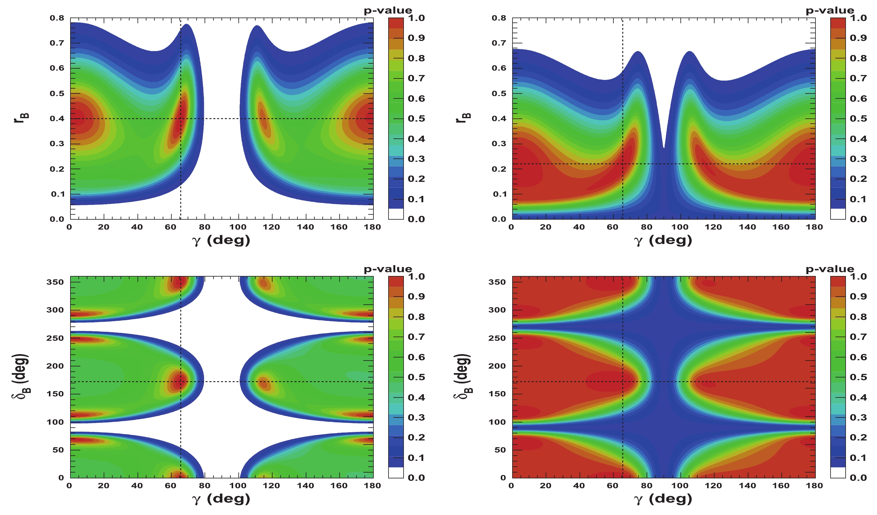
Figure F1. (color online) 2-D p-value profiles of nuisance parameters
${r_{B}}$ and${\delta_{B}}$ , for the Run 1 & 2 LHCb dataset, as a function of$\gamma$ . In each figure, the dashed black lines indicate the initial true values$\gamma=65.66^\circ$ (1.146 rad),${\delta_{B}}=171.9^\circ$ (3.0 rad), and${r_{B}}=0.4$ (left) and 0.22 (right) (w/o${B^0_s} \rightarrow {D^{*0}}\phi$ ).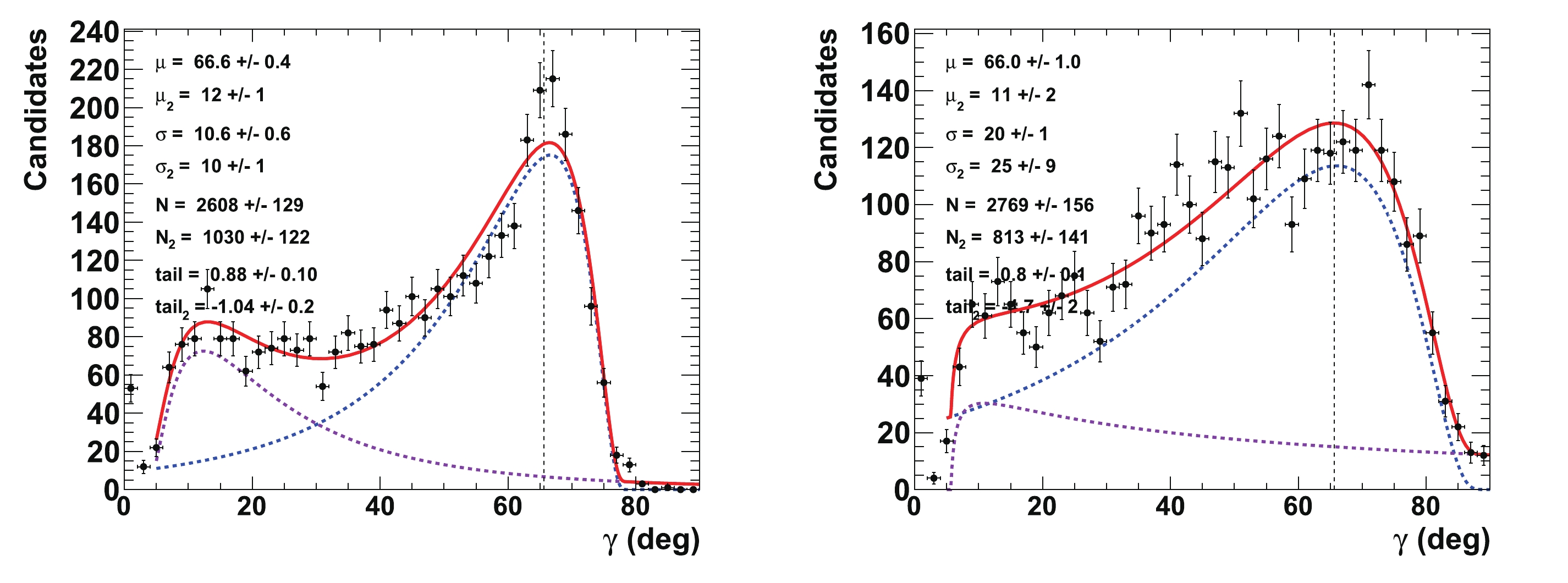
Figure F2. (color online) Fit to distributions of
$\gamma$ obtained from 4000 pseudoexperiments for Run 1 & 2 LHCb dataset. The initial configuration is$\gamma=65.66^{\circ}$ ,${r_{B}}=0.4$ (left) and 0.22 (right), and${\delta_{B}}=171.9^\circ$ (3 rad) (w/o${B^0_s} \rightarrow {D^{*0}}\phi$ ). The purple dashed curve represents the tails generated by the correlations with the nuisance parameters${r^{(*)}_{B}}$ and$\delta _B^{(*)}$ , whereas the blue dashed curve indicates the core part of the distribution, and the plain red line is the sum of the two components of the fit.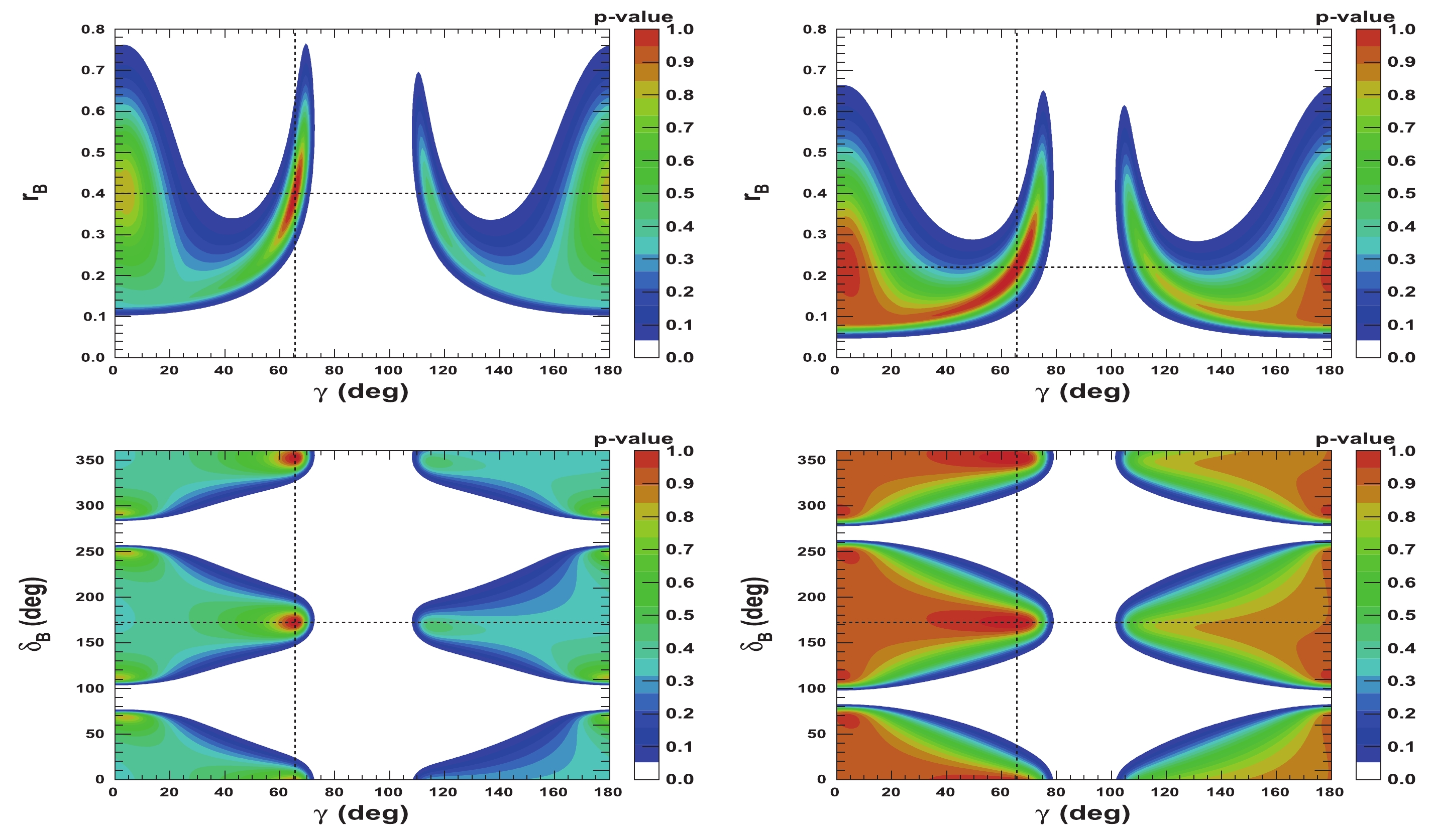
Figure F3. (color online) 2-D p-value profiles of nuisance parameters
${r_{B}}$ and${\delta_{B}}$ (Run$1-3$ LHCb) as function of$\gamma$ . In each figure, the dashed black lines indicate the initial true values$\gamma=65.66^\circ$ (1.146 rad),${\delta_{B}}=171.9^\circ$ (3.0 rad), and${\delta^*_{B}}=114.6^\circ$ (2.0 rad), as well as${r_{B}}=0.4$ (left) and 0.22 (right) (w/o${B^0_s} \rightarrow {D^{*0}}\phi$ ).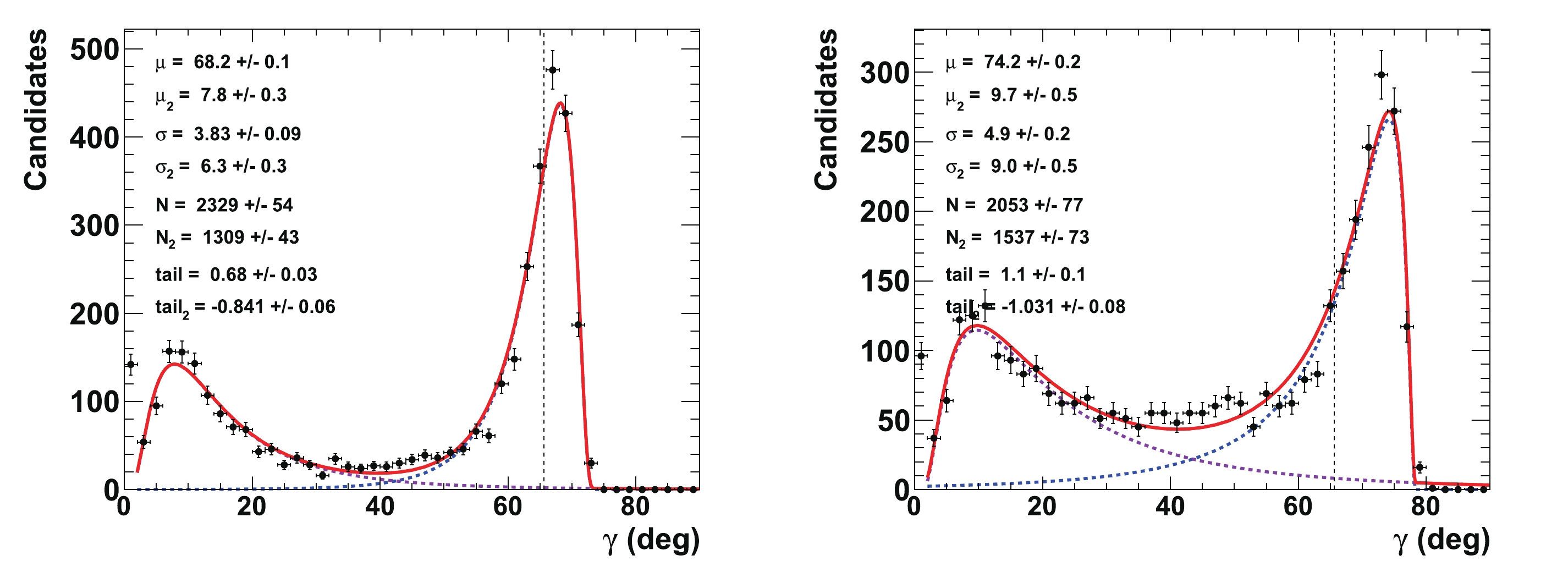
Figure F4. (color online) Fit to distributions of
$\gamma$ obtained from 4000 pseudoexperiments (Run$1-3$ LHCb). The initial configuration is$\gamma=65.66^{\circ}$ ,${r_{B}}=0.4$ (left) and 0.22 (right), and${\delta_{B}}=171.9^\circ$ (3 rad) (w/o${B^0_s} \rightarrow {D^{*0}}\phi$ ). The purple dashed curve represents the tails generated by the correlations with the nuisance parameters${r^{(*)}_{B}}$ and$\delta _B^{(*)}$ , whereas the blue dashed curve indicates the core part of the distribution, and the plain red line is the sum of the two components of the fit.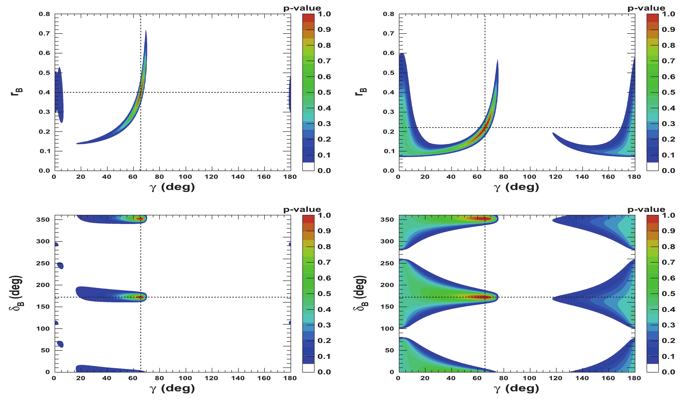
Figure F5. (color online) 2-D p-value profiles of nuisance parameters
${r_{B}}$ and${\delta_{B}}$ (full HL-LHC LHCb) as function of$\gamma$ . In each figure, the dashed black lines indicate the initial true values$\gamma=65.66^\circ$ (1.146 rad) and${\delta_{B}}=171.9^\circ$ (3.0 rad), as well as${r_{B}}=0.4$ (left) and 0.22 (right) (w/o${B^0_s} \rightarrow {D^{*0}}\phi$ ).
Figure F6. (color online) Fit to distributions of
$\gamma$ obtained from 4000 pseudoexperiments (full HL-LHC LHCb). The initial configuration is$\gamma=65.66^{\circ}$ ,${r_{B}}=0.4$ (left) and 0.22 (right), and${\delta_{B}}=171.9^\circ$ (3 rad) (w/o${B^0_s} \rightarrow {D^{*0}}\phi$ ). The purple dashed curve represents the tails generated by the correlations with the nuisance parameters${r^{(*)}_{B}}$ and$\delta _B^{(*)}$ , whereas the blue dashed curve indicates the core part of the distribution, and the plain red line is the sum of the two components of the fit. -
Untagged
$ {{B^0_s}}\rightarrow \tilde{D}^{(*)0}\phi $ decays provide another theoretically clean pathway to the measurement of the CKM-angle$ \gamma $ . By using the expected event yields for D decays on$ K\pi $ ,$ K3\pi $ ,$ K\pi{{\pi^{0}}} $ ,$ KK $ , and$ \pi\pi $ , we have demonstrated that a precision on$ \gamma $ of approximately$8^{\circ}$ to$ 19^{\circ} $ can be achieved with LHCb Run 1 & 2 data. With additional data, a precision on$ \gamma $ of$3^{\circ}-8^{\circ}$ can be achieved with the LHCb Run$ 1-3 $ dataset (23 fb-1 in 2025). Ultimately, a precision of the order of$2^{\circ}-7^{\circ}$ is expected with the full HL-LHC LHCb dataset (300 fb-1 in 2038). The asymptotic sensitivity is dominated by the possibly large correlations of$ \gamma $ with respect to the nuisance parameters$ {{r^{(*)}_{B}}} $ and$ {{\delta^{(*)}_{B}}} $ . The use of this method can improve our knowledge of$ \gamma $ from$ {{B^0_s}} $ decays and aid in understanding the discrepancy of$ \gamma $ between measurements with$ {{B^+}} $ and$ {{B^0_s}} $ modes.We are grateful to all members of the CKMfitter group for their comments and providing us with their private software based on a frequentist approach for computing the many pseudoexperiments performed for this study. In particular, we would like to thank J. Charles for his helpful comments on starting this analysis.
Study of the CKM angle γ sensitivity using flavor untagged $ {{B^0_s}} {\rightarrow} \tilde{{D}}^{{(*)0}} {\phi} $ decays
- Received Date: 2020-08-03
- Accepted Date: 2020-11-03
- Available Online: 2021-02-15
Abstract: A sensitivity study on the measurement of the CKM angle


 DownLoad: