Origin of hardening in spectra of cosmic ray nuclei at a few hundred GeV using AMS-02 data

Cosmic ray (CR) physics has entered a precision-driven era. More and more fine structures have been confirmed by a new generation of space-borne and ground-based experiments in recent years. For the spectra of CR nuclei, the most obvious fine structure is the spectral hardening at $ \sim $ 300 GeV, which has been observed by ATIC-2 [1], CREAM [2], and PAMELA [3].

The space-based Alpha Magnetic Spectrometer (AMS-02) experiment, which was launched in May 2011, has improved the measurement precision of CR fluxes by an order of magnitude [4]. To date, AMS-02 has released the spectra of different nuclear species, including the primary CR species (protons [5], helium (He), carbon (C), oxygen (O) [6], neon (Ne), magnesium (Mg), and silicon (Si) [7]), secondary CR species (lithium (Li), beryllium (Be), and boron (B) [8]), and hybrid CR species (nitrogen (N) [9]). All these CR species show spectral hardening in the region of $ 100-1000 $ GeV, which confirms the previous observational results. Moreover, it shows that the spectra of secondary nuclei harden even more than those of primary nuclei at a few hundred GeV. The spectral index of the N spectrum hardens rapidly at high rigidities and becomes identical to the spectral indices of primary He, C, and O CRs.

This spectral hardening phenomenon has been studied in many previous works. Generally speaking, the spectral hardening could come from: (i) primary source acceleration (see e.g. Refs. [10-21]); (ii) propagation (see e.g. Refs. [16, 19, 20, 22-31]); or (iii) the superposition of different kinds of sources, such as different populations of sources or local and distant sources (see e.g. Refs. [28, 31-44]). Based on the galactic CR diffusion model, all these scenarios could provide good fits to specific data sets. No scenario has stood out yet.

Although most previous studies use a uniform injection spectrum for all the primary CR nuclei, or employ an independent injection spectrum for protons because of the proton-to-helium ratio anomaly [24], some pioneering works (such as Refs. [17, 19, 20]) introduce different injection spectra for different primary CR nuclei. Considering the different data sets and propagation models used in these works, it is natural that the injection spectral parameters of the same primary component are different. However, all these works show different primary CR injection spectral parameters for different primary CR species. This result should be given more attention. In particular, the break rigidities and the spectral index differences less than and greater than the break of the species could directly provide important information about the origin of the hardening. The observed CR spectra are physically produced by the injection spectra and the propagation process; even so, it is helpful to analyze all the observed/propagated AMS-02 spectra directly via a uniform method, which could provide us some robust conclusions about the primary source acceleration and the propagation of CRs (The recent works which focus on the injection spectra (before propagation) based on specific propagation models can be found in Refs. [17, 19, 20] and related references therein).

In the following, we analyze the spectra in Section II. Discussion is given in Section III, and conclusions and outlook are presented in Section IV.

We focus on the spectral hardening at a few hundred GeV. Therefore, data points with rigidity less than 45 GeV are not used in this work; they are also affected by solar modulation and cannot be fitted by a simple broken power law. When the rigidity is greater than 45 GeV (up to a few thousand GeV), all the spectra can be well fitted by a broken power law or smooth broken power law [5-9]. Considering the precision of the AMS-02 data, it is unnecessary to employ a smoothing factor to describe the spectral index transformation^②.

Consequently, the following formula is used to describe each of the AMS-02 spectra for CR nuclei (including primary, secondary and hybrid CR species) when the rigidity is greater than 45 GeV:

where F is the CR flux, N is a normalization constant, $ \nu_{1} $ and $ \nu_{2} $ are the spectral indexes less than and greater than the break rigidity $ \,R_{\mathrm{br}} $ , respectively, and $ \mathrm{i} $ denotes the species of nuclei. The errors used in our fitting are the quadratic sum of statistical and systematic errors.

The Markov Chain Monte Carlo (MCMC) algorithm is employed to determine the posterior probability distribution of the spectral parameters belonging to different CR species (The PYTHON module emcee [45] is employed to perform the MCMC sampling. Some such examples can be referred to Refs. [13, 16, 46] and references therein). The best-fit values and the allowed intervals from the 5th to the 95th percentile of the parameters $ \nu_1 $ , $ \nu_2 $ , $ \,R_{\mathrm{br}} $ , and $ \Delta \nu \equiv \nu_2 - \nu_1 $ are listed in Table 1, together with the reduced $ \chi^2 $ of each fitting^④. The best-fit results and the corresponding residuals of the primary, secondary, and hybrid CR species are shown in Figs. A1, A2, and A3 of Appendix A, respectively.

Species	$\nu_1$	$\nu_2$	$R_{\rm{br} }/\mathrm{GV}$	$\Delta \nu$	$\chi^2 / \mathrm{d.o.f}$
proton	−2.815 [−2.823,−2.806]	−2.71 [−2.76,−2.62]	379 [300, 544]	0.10 [0.06,0.19]	1.21/27 = 0.045
Helium	−2.725 [−2.733,−2.715]	−2.62 [−2.65,−2.56]	331 [281, 448]	0.10 [0.07,0.16]	2.65/28 = 0.095
Carbon	−2.74 [−2.76,−2.72]	−2.64 [−2.68,−2.59]	202 [148, 299]	0.10 [0.05,0.15]	5.26/28 = 0.188
Oxygen	−2.696 [−2.712,−2.680]	−2.49 [−2.63,−2.27]	664 [488, 964]	0.21 [0.07,0.43]	1.91/28 = 0.068
Neon	−2.74 [−2.76,−2.72]	−2.33 [−2.61,−1.98]	670 [405, 995]	0.41 [0.13,0.76]	6.01/27 = 0.222
Magnesium	−2.74 [−2.76,−2.72]	−2.61 [−2.79,−2.31]	410 [287, 978]	0.13 [-0.06,0.42]	4.68/27 = 0.173
Silicon	−2.71 [−2.73,−2.69]	−2.79 [−3.24,−2.51]	922 [491, 988]	-0.08 [-0.53,0.21]	7.21/27 = 0.267
Lithium	−3.18 [−3.20,−3.10]	−2.98 [−3.01,−2.72]	123 [112, 351]	0.20 [0.14,0.41]	22.51/27 = 0.834
Beryllium	−3.13 [−3.16,−3.08]	−2.95 [−3.06,−2.77]	199 [173, 438]	0.17 [0.04,0.34]	18.29/27 = 0.677
Boron	−3.10 [−3.13,−3.07]	−2.84 [−2.96,−2.66]	275 [194, 422]	0.26 [0.14,0.44]	11.42/27 = 0.430
Nitrogen	−2.93 [−2.95,−2.87]	−2.66 [−2.70,−2.34]	208 [188, 454]	0.27 [0.21,0.56]	10.96/27 = 0.406

Table 1.  Fitting results of spectral parameters for different nuclear species. Best-fit values and allowed 5th to 95th percentile intervals (in square brackets) are listed for each of the parameters.

Generally speaking, the $ \chi^2 $ s of primary CR species are smaller than the other 2 types of species, due to the dispersion of the data points (especially in the high rigidity region) in the latter cases.

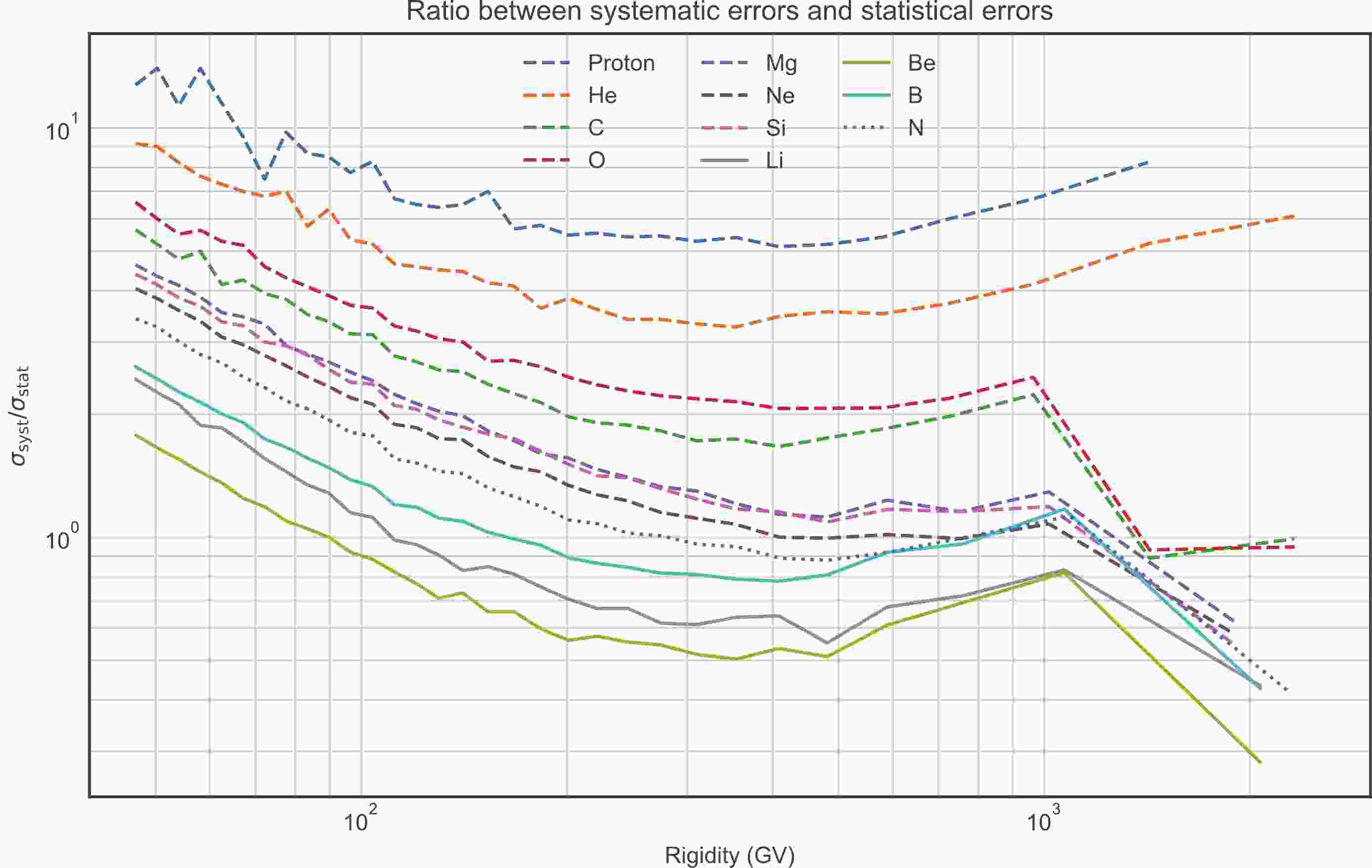
Here, one should note that the $ \chi^2/\mathrm{d.o.f} $ of the best-fit result for the primary species (especially for protons, helium and oxygen) are much smaller than 1.0, which indicates an improper treatment of the data errors in the fitting process. In the AMS-02 data [5-9], we find that the systematic errors are always dominant (see Fig. 1), which will lead to smaller $ \chi^2 $ if we ignore the energy correlations for them. Figure 1 shows the ratio between the systematic errors ( $ \sigma_{\mathrm{syst}} $ ) and statistical errors ( $ \sigma_{\mathrm{stat}} $ ) with the variation of rigidity. It is clear that the species with the largest 3 $ \sigma_{\mathrm{syst}}/\sigma_{\mathrm{stat}} $ values (proton, helium and oxygen) correspond to the smallest 3 $ \chi^2 / \mathrm{d.o.f.} $ values in Table 1. In such a case, we need the correlation matrix of systematic errors of AMS-02 data if we want reasonable $ \chi^2 / \mathrm{d.o.f.} $ s for the fitting results. Unfortunately, the AMS-02 collaboration does not provide correlation matrices of systematic errors. Consequently, the values of $ \chi^2/\mathrm{d.o.f} $ in Table 1 do not have the absolute meaning of goodness-of-fit. Further data analysis needs more information about the systematic errors. Some detailed discussions of this topic can be found in Refs. [47-49].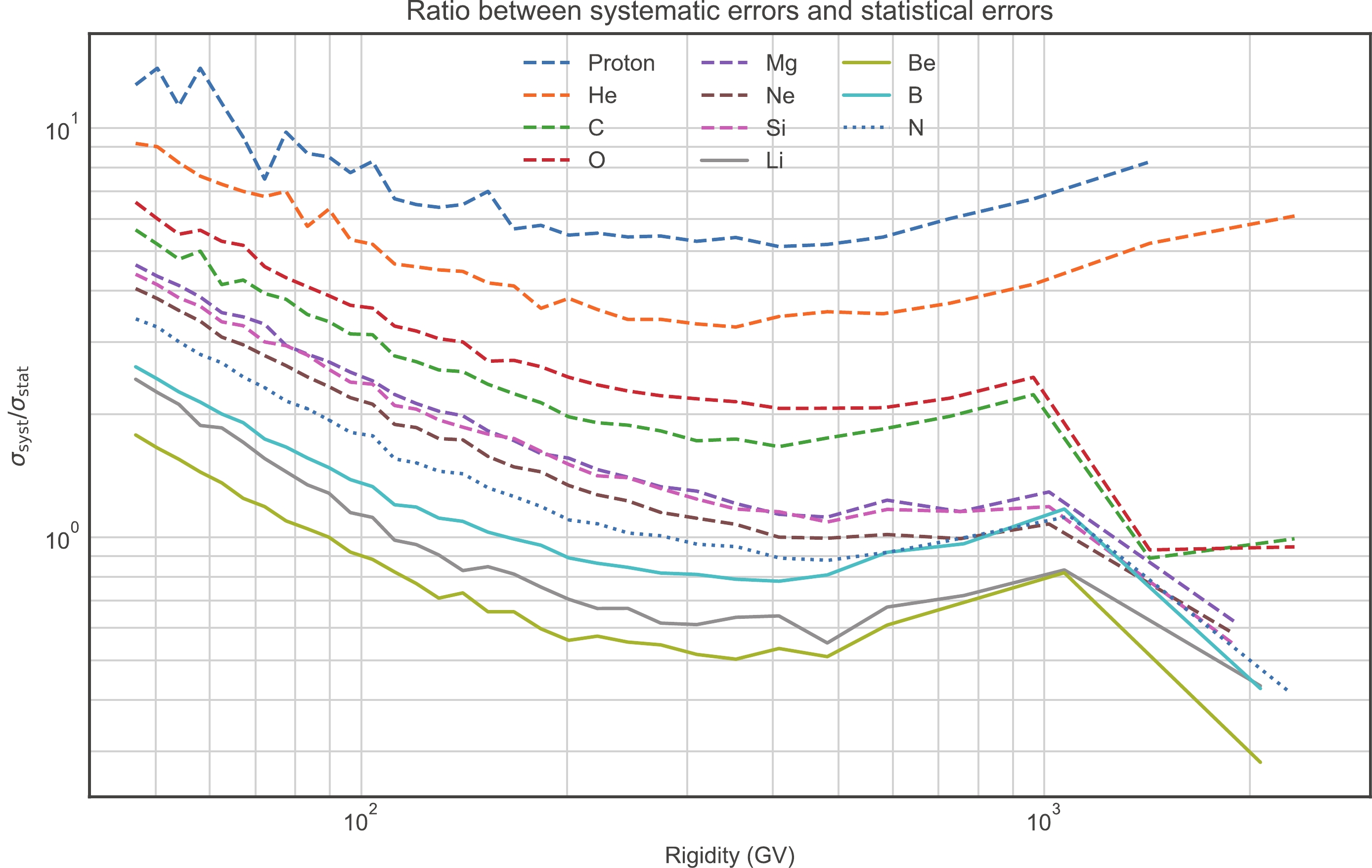

Figure 1.  (color online) Ratio between systematic errors and statistical errors $ \sigma_{\mathrm{syst}}/\sigma_{\mathrm{stat}} $ with variation of rigidity for different species. Primary CR species are represented by dashed lines, secondary CR species by solid lines, and the hybrid CR species is represented by a dotted line.

In order to get a clear representation of the fitting results, we use a boxplot^⑤ to show all the distributions of $ \nu_1 $ , $ \nu_2 $ , $ \,R_{\mathrm{br}} $ and $ \Delta \nu $ in Fig. 2.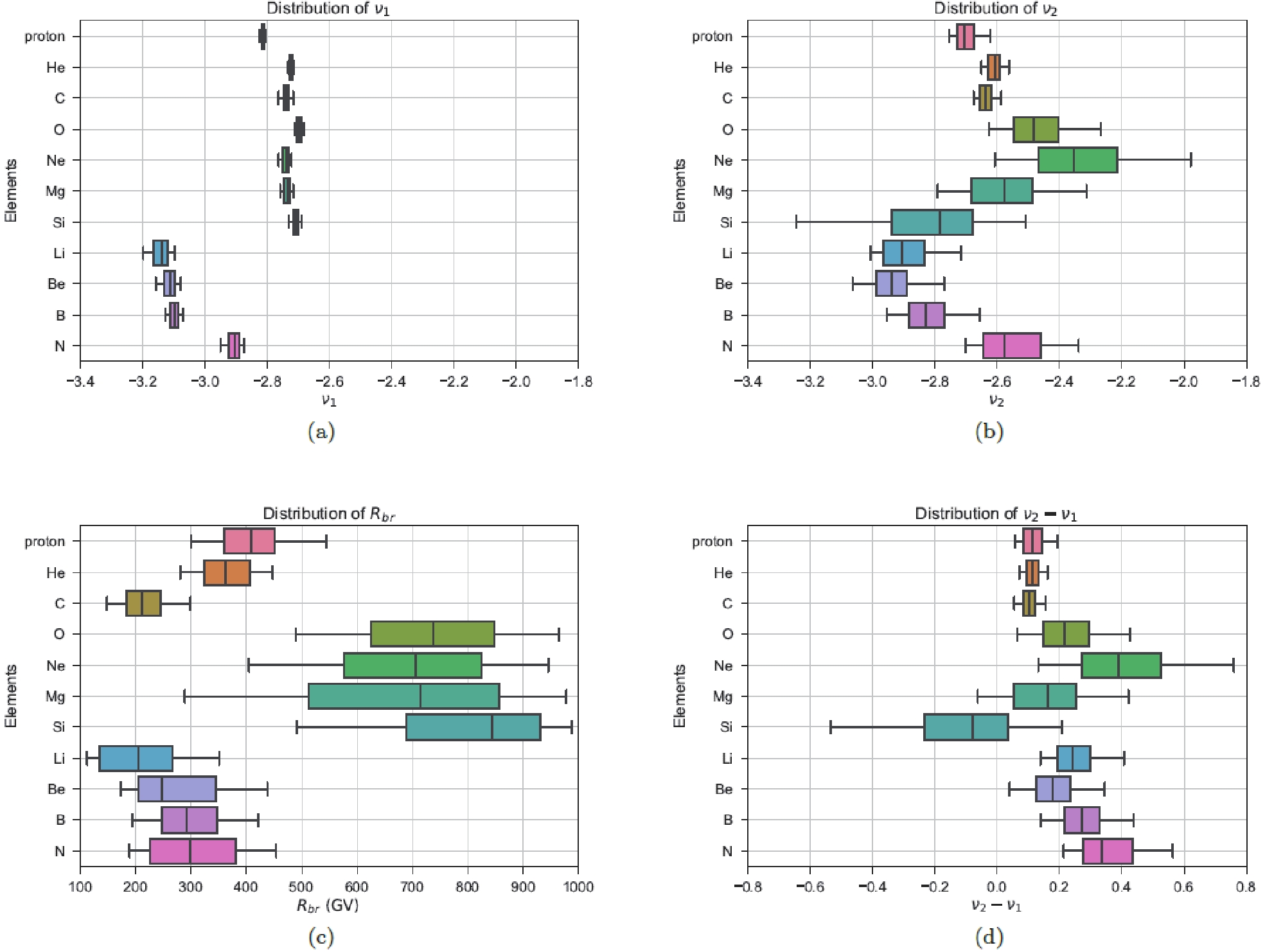

Figure 2.  (color online) Boxplots for $ \nu_1 $ , $ \nu_2 $ , $ \,R_{\mathrm{br}} $ , and $ \nu_2-\nu_1 $ . The band inside each box shows the median value of the dataset, the box shows the quartiles, and the whiskers extend to show the rest of the distribution which are edged by the 5th and 95th percentile.

In Fig. 2, it is obvious that the values of $ \nu_1 $ can be divided into 3 groups, which correspond to the primary, secondary, and hybrid CR species. As the transition between the primary and secondary CR species, it is reasonable that the hybrid species (N) has a value of $ \nu_1 $ between the other 2 species. Moreover, the proton has a distinct value of $ \nu_1 $ compared with other CR primary species. More interestingly, $ \nu_1 $ for O and Si (especially O) is larger than for other species. Based on the above principle of classification, O and Si CR spectra should have the fewest secondary components, while all the other primary nuclear species (especially the proton) should have considerable secondary components which could influence the spectral index significantly in this rigidity region (such as C, which has about 20% secondary component in its flux [50]). Another explanation for the different $ \nu_1 $ values of primary CR species is their different primary source injections. In such a case, it might be straightforward to ascribe the specific $ \nu_1 $ of the proton to its charge-to-mass ratio, but it is difficult to find a universal mechanism to explain the different $ \nu_1 $ values for other primary species.

In the subfigure (b) of Fig. 2, the uncertainties of $ \nu_2 $ are larger than those of $ \nu_1 $ , because there are fewer data points with larger uncertainties in the high rigidity region in the AMS-02 CR spectra. The 3 clear groups in Fig. 2(a) are replaced by complicated relationships. Different from the relationships of $ \nu_1 $ for primary species, the $ \nu_2 $ of Ne, Mg, and Si have even larger uncertainties and cover a large interval, from that of the primary species (protons, He, C, and O) to the secondary species (Li, Be, and B). The $ \nu_2 $ of N is somewhat consistent with the primary component dominating the N spectra in the high rigidity region [9].

In Fig. 2(c), it is shown that the values of $ \,R_{\mathrm{br}} $ can be divided into 2 groups: proton, He, C, Li, Be, B, and N in one group; and O, Ne, Mg, and Si in another group. As the daughter species of C, N (The break here is mainly determined by its primary component [9]), O, Ne, Mg, and Si, the secondary species (Li, Be, and B) have similar $ \,R_{\mathrm{br}} $ values to C and N, but show systematically different $ \,R_{\mathrm{br}} $ intervals from O, Ne, Mg, and Si. For the primary CR species, it is interesting that the $ \,R_{\mathrm{br}} $ values of the proton, He, C, and N are different from those of O, Ne, Mg, and Si. The above different rigidities of the breaks deny the propagation scenario, which introduces a unique break in the diffusion coefficient to reproduce the hardening in all these CR species.

In the subfigure (d) of Fig. 2(d), the values of $ \Delta \nu $ inherit large uncertainties from $ \nu_2 $ , especially for N, O, Ne, Mg, and Si. As in the case of $ \nu_2 $ , the $ \Delta \nu $ values of Ne, Mg, and Si have even larger uncertainties and cover a large interval, from that of the primary species (proton, He, C, and O) to the secondary species (Li, Be, and B). Additionally, the $ \Delta \nu $ of Si even has a negative best-fit value (In the Figure 5 of Ref. [7], AMS-02 collaboration get a positive $ \Delta \nu $ for the Si spectrum, because they use a power law function with same spectral indexes and break to fit the spectra of Ne, Mg, and Si simultaneously (with different normalization factors), while we use independent power law functions to fit the spectra). Moreover, it shows that the $ \Delta \nu $ values of some primary species whose spectra have relatively small uncertainties (proton, He, and C) are systematically smaller than those of the secondary species (Li, Be, and B), which is why the AMS-02 spectral data favor a break in the diffusion coefficient index rather than a break in the primary source injection (see e.g. Refs. [18, 27]). However, if we note how much the flux of the parent species (mainly from C, N, and O) contributes to the daughter species (Li, Be, and B), an absolutely different conclusion can be obtained.

The CR flux of Li has the ratio of contribution from its parent species (Of course, Ne, Mg, Si, and Fe also contribute to the flux of Li, Be, and B. Here, we just list the dominating parents species, more details can be found in Ref. [50]) of $ \mathrm{C}:\mathrm{N}:\mathrm{O} \simeq 0.931:1.203:1.672 $ ; for Be, $ \mathrm{C}:\mathrm{N}:\mathrm{O} \simeq 1.178:1.215:2.300 $ ; and for B, $ \mathrm{C}:\mathrm{N}:\mathrm{O} \simeq 0.956:0.864:1.265 $ (see Table IV in Ref. [50]). The contributions from the N and O flux are about 2 to 3 times larger than that from the C flux. At the same time, the ranges of $ \Delta \nu $ of Li, Be, and B are perfectly covered by those of C, N, and O (especially N and O). All of the evidence shows that the parents and their daughter species have some ranges of $ \Delta \nu $ , and it is unnecessary to produce an “extra hardening” in the daughter species' spectra via introducing a break in the diffusion coefficient. The conclusions obtained in some previous works (such as Refs. [18, 27]) can be explained as: (i) just using the B/C ratio to check the propagation models, while the $ \Delta \nu $ of C is coincidentally half of that of B; (ii) the use of proton and helium data with small uncertainties (which also have relatively small values of $ \Delta \nu $ like that of C) dilutes the impacts of the real parent species (Especially N and O. In a recent work Ref. [21], the authors use the primary spectra of C and O to reproduce the secondary spectra of Li, Be, and B successfully without adding an extra break in the diffusion coefficient, which can be naturally explained by the above discussions).

It is shown that not only are the values of $ \nu_1 $ , $ \nu_2 $ and $ \Delta \nu $ different for different primary CR species, but the relationships of $ \nu_1 $ (low rigidity region) and $ \nu_2 $ (high rigidity region) between different primary species are also obviously different. In particular, the CR spectra of Ne, Mg, and Si represent different properties compared with other primary species, which infers that they might come from different sources in a different rigidity region.

Consequently, if the spectral hardening comes from primary source acceleration or propagation, it is necessary to first introduce independent primary source injection for each of the primary CR species. For the propagation case, independent breaks and relevant diffusion coefficient indexes are also needed to reproduce the observed spectra precisely. However, except for the proton, which has a different charge-to-mass ratio, there is no clear physical motivation for other primary CR nuclei to have different source injections, let alone independent breaks and indexes in their diffusion coefficients.

Moreover, considering that the flux of B is mainly contributed by N and O rather than C (whose flux itself has about 20% secondary component), it is a more reasonable choice to use B/O (or Li/O, Be/O) ratio to check the propagation models.

In summary, the spectra of CR nuclei observed by AMS-02 show complicated relationships in the spectral indexes less than and greater than the rigidity of the hardening (break) at a few hundred GeV between the primary CR species. This disfavors the spectral hardening simply coming from primary source acceleration or propagation, if we adhere to the principles of naturality and simplicity for our CR models.

Fortunately, the superposition of different kinds of sources could naturally reproduce all the spectral indexes ( $ \nu_1 $ and $ \nu_2 $ ) and breaks ( $ \,R_{\mathrm{br}} $ ) for different CR nuclear species with a simple and natural assumption that each kind of source could have a unique spectral index for all the primary source injection, and have different element abundances than other kinds of source (see e.g. Refs. [32, 43, 44]). Considering the different kinds of potential CR sources (such as the different populations of supernovae), this assumption is consistent with real astrophysical situations. In this scenario, the values of $ \nu_1 $ indicate that one kind of source dominates in this rigidity region, and the values of $ \nu_2 $ and $ \,R_{\mathrm{br}} $ are the results of superposition of other kind of sources with different spectral indexes and element abundances which have considerable flux in this rigidity region (see e.g. Refs. [43, 44]).

Because of the small number and large uncertainties of the data points greater than the break rigidity, the fitting values of $ \nu_2 $ and $ \,R_{\mathrm{br}} $ (which is closely related to the detailed properties of the second type of sources) have large uncertainties. Furthermore, the differences in systematics between different experiments (mainly from the energy calibration process) prevent precise fitting of a collection of data from more than one experiment, covering different rigidity regions. As a result, spectra of CR nuclei from a single experiment (such as DAMPE) are needed to do cross checks and reveal the properties of the different kinds of sources in future.

The author would like to thank the referees for their valuable and detailed suggestions, which led to great progress in this work.

Note that in the lower panels of the subfigures in Figs. A1, A2, and A3, $ \sigma_{\mathrm{eff}} $ is defined as

Figure A1.  (color online) Ratio between systematic errors and statistical errors $ \sigma_{\mathrm{syst}}/\sigma_{\mathrm{stat}} $ with the variation of rigidity for different species. The primary CR species are represented in dashed lines, the secondary CR species are represented in solid lines, and the hybrid CR species is represented in dotted line.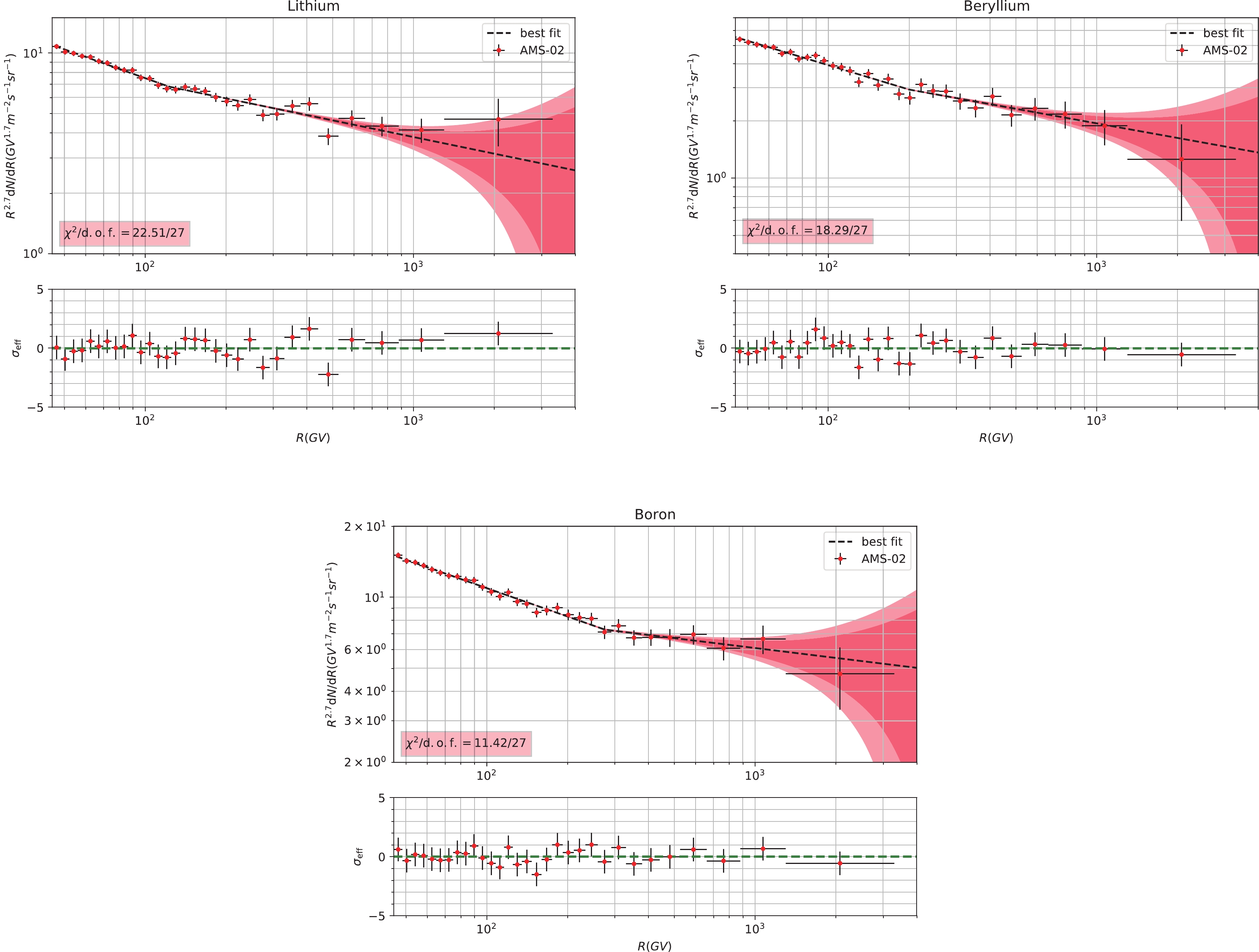

Figure A2.  (color online) Fitting results and corresponding residuals to the primary CR nuclei spectra (proton, He, C, O, Ne, Mg, and Si). The 2 $ \sigma $ (deep red) and 3 $ \sigma $ (light red) bounds are also shown in the subfigures. The relevant reduced $ \chi^2 $ of each spectrum is given in the subfigures as well.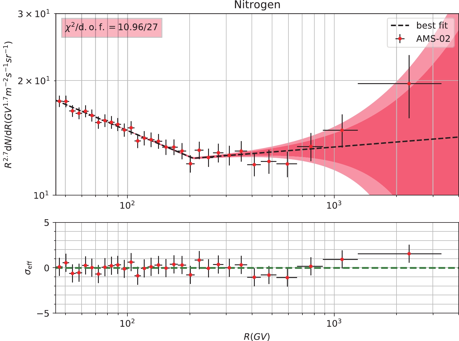

Figure A3.  (color online) Fitting results and corresponding residuals to the hybrid CR nuclei spectra (N). The 2 $ \sigma $ (deep red) and 3 $ \sigma $ (light red) bounds are also shown in the subfigures. The relevant reduced $ \chi^2 $ of each spectrum is given in the subfigures as well.

where $ f_\mathrm{obs} $ and $ f_\mathrm{cal} $ are the points which come from the observation and model calculation, and $ \sigma_\mathrm{stat} $ and $ \sigma_\mathrm{syst} $ are the statistical and systematic standard deviations of the observed points. This quantity can clearly show us the deviations between the best-fit result and observed values at each point, based on its uncertainty.