


 Abstract
 HTML
HTML Reference
 Related
 PDF
PDF


-
The Cabibbo-Kobayashi-Maskawa (CKM) matrix can accommodate CP violation (CPV) in a natural way with a complex phase in the quark mixing sector [1, 2]. Experimentally, CPV has been observed in the meson sector, first in the K meson [3-5], subsequently in the B meson [6-11] and most recently in charm meson decays [12]. All results to date are consistent with the predictions of the CKM mechanism in the Standard Model (SM).
However, the origin of CPV has remained an unsolved problem, as it is not clear whether the CKM mechanism is the unique source. The matter-antimatter asymmetry of the universe [13, 14] indicates that there must be non-SM CPV sources, and such additional sources are indeed incorporated in many extensions of the SM [15, 16]. Currently, CPV has not been observed in the lepton sector, and any significant observation would be a clear indication of physics beyond the SM. In an intriguing scenario [17], baryogenesis is argued to be mainly driven by leptogenesis, and then CPV is required in leptodynamics. Thus, exploration of CPV in the lepton sector provides a different and complementary landscape, at least. In the lepton sector,
$ \tau $ decay is a good place to seek for CPV either within or beyond the SM [18-22], since it has abundant hadronic decay channels with sizable branching ratios. Furthermore, half of the matrix element is purely electroweak and the hadrons involved are generated by quark-antiquark pairs, such that they are factorized, avoiding the complications of pure hadronic decay.In this paper, we will discuss the specific channel
$ \tau^{-}\to K_{S}\pi^{-}\nu_{\tau} $ and concentrate on CPV and related New Physics (NP) searches. This channel is also of great importance for the measurements of form factors and extraction of the$ |V_{us}| $ element in the CKM matrix. It also has rich intermediate resonances which provide an important playground for non-perturbative QCD studies. Experimentally, a rich source of$ \tau $ leptons comes from electron-positron colliders, and the physics programs related to$ \tau $ decays are usually performed at a B-factory or Z-factory. There are a lot of prospects for the potential of$ \tau $ decays at future such factories [23]. However,$ \tau $ decays are rarely investigated in the tau-charm energy region, due to the low statistics available and the difficulty in reconstruction. A feasibility study of$ \tau $ decays in the tau-charm region will be of great importance to complete the global picture of whole$ \tau $ physics. The proposed STCF [24] in China is designed to have a peak luminosity of$ >0.5\times10^{35} $ cm$ ^{-2} $ s$ ^{-1} $ at$ \sqrt{s} = 4 $ GeV. It is a symmetric electron-positron beam collider designed to provide$ e^{+}e^{-} $ interactions at c.m. energy$ \sqrt{s} $ from 2.0 to 7.0 GeV. The$ \tau $ leptons are selected via the process$ e^{+}e^{-}\to\tau^{+}\tau^{-} $ , where the cross-section of$ e^{+}e^{-}\to\tau^{+}\tau^{-} $ peaks at 3.5 nb, around$ \sqrt{s} = $ 4.26 GeV [25]. The number of$ \tau $ pairs produced at STCF is estimated to be$ 3.5\times10^{9} $ , with an expected integrated luminosity of 1 ab$ ^{-1} $ per year.This paper is organized as follows. In Sec. II, we elaborate the physical significance of investigating the channel
$ \tau^{-}\to K_{S}\pi^{-}\nu_{\tau} $ . In Sec. III, the detector concept for STCF is introduced, as well as the Monte Carlo (MC) samples used for this study. The event selection for the signal process and detector optimization are presented in Sec. IV and Sec. V respectively. Section VI discusses the results and Sec. VII gives our conclusion. -
Within the SM, there is no direct CPV in hadronic
$ \tau $ decays at tree level in weak interactions. However, the well-measured CPV in$ K_{L}\to\pi^{\mp}l^{\pm}\nu $ $ (l = e,\mu) $ produces a difference in$ \Gamma(\tau^{+}\to K_{L}\pi^{+}\bar{\nu}_{\tau}) $ vs.$ \Gamma(\tau^{-}\to K_{L}\pi^{-}{\nu_{\tau}}) $ due to the$ K^0-\bar K^0 $ oscillation. The same asymmetry also appears in$ \Gamma(\tau^{+}\to K_{S}\pi^{+}\bar{\nu}_{\tau}) $ vs.$ \Gamma(\tau^{-}\to K_{S}\pi^{-}{\nu_{\tau}}) $ , and is calculated to be [26, 27]:$ \begin{aligned}[b] A_{CP}(\tau^-\to K_{S}\pi^-\nu_{\tau}) =& \frac{\Gamma(\tau^+\to K_{S}\pi^+\bar\nu_{\tau})-\Gamma(\tau^-\to K_{S}\pi^-\nu_{\tau})}{\Gamma(\tau^+\to K_{S}\pi^+\bar\nu_{\tau})+\Gamma(\tau^-\to K_{S}\pi^-\nu_{\tau})} \\ = &(0.33\pm0.01)\%. \end{aligned} $

(1) Experimentally, the BaBar experiment has found evidence for CPV in
$ \tau $ decays [28]:$ A_{CP}(\tau^-\to K_{S}\pi^-\nu_{\tau}[\geqslant 0\pi^{0}]) = (-0.36\pm0.23\pm0.11)\%, $

(2) and there is a
$ 2.8 $ standard deviation difference from the theoretical prediction in Eq. (1). It should be noted that the$ K^0-\bar K^0 $ oscillation leads to the same value of CPV for inclusion of any$ \pi^0 $ s in$ \tau $ decays from the SM prediction.Motivated by the above CPV disagreement, various NP scenarios have been proposed, e.g. introducing a non-standard tensor interaction [29, 30]. In Ref. [30], a very large angular-weighted CPV is predicted additionally, with such a tensor interaction. However, those conclusions are questioned in Ref. [31], where the authors point out the tensor contributions used in Refs. [29, 30] are overestimated due to the lack of the well-known Watson theorem of final-state interactions, resulting in very large values of the imaginary parts of the Wilson coefficients to explain the
$ CP $ anomaly; those large values of Wilson coefficients contradict the bound from the neutron electric dipole moment (EDM) and$ D-\bar D $ mixing (unless NP occurs below the electroweak breaking scale). The standpoint of Ref. [31] is adopted later in Refs. [32, 33], and especially, Ref. [33] finds that once the combined constraints from the branching ratio and decay spectrum are imposed, it is hard to explain the experimental values of CPV. But again, Ref. [31] is questioned by the authors of Ref. [34] – they point out that the tensor operator used in Ref. [31] corresponds only to a specific way of imposing gauge invariance, and instead, introducing a new type of tensor operator could account for the$ CP $ anomaly while evading bounds from the neutron EDM and keeping the extraction of$ |V_{us}| $ from exclusive$ \tau $ decay unaffected. In brief, BaBar's CPV observables lead to a series of theoretical discussions, and those theoretical discussions are in a state of confusion. Therefore, a new measurement on the experimental side is essential to approach any conclusive statement on the NP signal. We stress the importance of precision here.Moreover, as discussed in Ref. [19], probing
$ A_{CP}(\tau^{-}\to [K\pi]^{-}\nu_{\tau}) $ ,$ A_{CP}(\tau^{-}\to [K 2\pi]^{-}\nu_{\tau}) $ and$ A_{CP}(\tau^{-}\to $ $ [K3\pi]^{-}\nu_{\tau}) $ separately can help to establish the existence of new dynamics, since the global CPV as expressed in Eq. (2) is often much reduced, and one needs to understand the basis of the observed data on$ \tau^{-}\to K_{S}\pi^{-}\nu_{\tau}[\geqslant 0\pi^{0}] $ vs.$ \tau^{-}\to [K\pi]^{-}\nu_{\tau} $ ,$ \tau^{-}\to [K 2\pi]^{-}\nu_{\tau} $ and$ \tau^{-}\to [K3\pi]^{-}\nu_{\tau} $ . In the SM, the same CPV holds for decays including any number of$ \pi^0 $ mesons, due to the sole source from$ K^0-\bar K^0 $ oscillation. However, the situation will change in the presence of NP. For example, the two-Higgs doublet model has been used to show its influence on the different observable sets for the channels$ \tau^{-}\to K \pi^{-} \pi^{0} \nu_\tau $ and$ \tau^{-}\to K \pi^{-} \nu_\tau $ [35, 36]. Certainly, a more complicated impact of resonances appears in the multibody channels, and more data is needed in this case. We also note that in four- and five-body decays, one can also access CPV by T-odd observables [37-39].Apart from the above BaBar measurement, the CLEO [40] and Belle [41] experiments have also focused on the CPV that could arise from a charged scalar boson exchange [42]. This type of CPV can be detected by measuring the
$ \tau^{\pm} $ decay angular distributions. The CPV is found to be compatible with zero with a precision of$ {\cal{O}}(10^{-3}) $ [41]. However, current experimental sensitivity cannot make a conclusion on the CPV from$ \tau $ decay, due to the large uncertainty. Therefore, a higher-precision result is required to hunt for signals of NP. At Belle II, CPV is studied in the angular distribution of$ \tau^{-}\to K_{S}\pi^{-}\nu_{\tau} $ decays, and the precision is expected to be$ \sqrt{70} $ times improved with a 50 ab$ ^{-1} $ data sample [43].In order to capture a faint NP signal, or instead, to constrain a NP model, accurate knowledge of the form factor is also an essential input [30, 32]. The process
$ \tau^{-}\to K_s\pi^{-}\nu_{\tau} $ decay in the SM is described by vector and scalar form factors. The vector form factor receives mainly the contribution of$ K^{*}(892) $ , while$ K^{*}(1410) $ is needed in the higher-energy region tail. For the scalar form factor, there is no clear dominance of a single resonance. Currently the most sophisticated theoretical description of the form factors is obtained by the model-independent dispersive representation, imposing constraints from chiral symmetry and their asymptotic QCD behavior [44-46]. However, other descriptions are available [36, 47]. In Ref. [36], the form factors are calculated up to one-loop level using the chiral Lagrangian. The resulting shape differs from the dispersive one in Ref. [44]. Such a difference may be attributed to the perturbative vs. non-perturbative treatment. Reference [47] aims to achieve a satisfactory description of experimental data in a phenomenological way, and then a superposition of Breit-Wigner functions is used. As already commented in Ref. [31], the resulting phase does not vanish at threshold and also violates the Watson theorem before the inelasticity sets in. In short, the shapes of the P-wave form factor agree, while the S-wave shapes can differ dramatically in different model calculations. However, from a pragmatic point of view, all these variants of form factor could describe the data for the total mass spectrum almost equally well. A partial-wave analysis will certainly help to pin down this issue, which again needs more high-quality data. This point has been noted by the Belle collaboration [47]: in future, more data on the invariant mass spectrum of$ K_s\pi $ combined with angular analysis will elucidate the nature of the scalar form factor and check various theoretical approaches. At STCF, high statistics of$ \tau^{-}\to K_{S}\pi^{-}\nu_{\tau} $ can put strong constraints on the vector and scalar form factors. Meanwhile, the precision in the determination of the form factor parameters can be improved.On the other hand,
$ |V_{us}| $ can be extracted from the measurement of the$ \tau^{-}\to K_{S}\pi^{-}\nu_{\tau} $ decay. Indeed, the decay rate of$ \tau^{-}\to K_{S}\pi^{-}\nu_{\tau} $ can be expressed as [48]:$ \Gamma = G^{2}_{F}NC^{2}_{K,\tau}S_{EW}(|V_{us}|f^{K^{0}\pi^-}_+(0))^{2}I_{K}(1+\delta_{EM}+\delta_{SU(2)})^{2}, $

(3) where N is a normalization coefficient (
$ N = m^{3}_{\tau}/(48\pi^{3}) $ ),$ G_{F} $ is the Fermi constant,$ C_{K,\tau} $ is the Clebsch-Gordan coefficient,$ I_{K} $ is the phase space integrals,$ S_{EW} $ is the electroweak short-distance,$ \delta_{EM} $ is the electromagnetic long-distance,$ \delta_{SU(2)} $ is the isospin breaking corrections, and$ f^{K^{0}\pi^{-}}_{+}(0) $ is the form factor at zero momentum transfer. According to the above equation, the measurement of$ |V_{us}| $ requires: i) accurate measurement of$ \Gamma $ ; ii) precise calculation of$ I_{K} $ ; iii) good knowledge of the radiative corrections, which are$ S_{EW} $ ,$ \delta_{EM} $ and$ \delta_{SU(2)} $ ; and iv) a determination of the value of$ f^{K^{0}\pi^{-}}_{+}(0) $ . In general, with higher precision for$ \tau^{-}\to K_{S}\pi^{-}\nu_{\tau} $ branching fraction measurements, the error on$ |V_{us}| $ will be reduced [49].In short, the physical importance of measuring
$ \tau^{-}\to K_{S}\pi^{-}\nu_{\tau} $ is discussed from three aspects: i) probing the CPV of this process and testing several NP scenarios; ii) the resonance parameters (mass and width) can also be determined, which is itself an important topic of the hadron spectrum, assisting us to understand more of the strong impact of intermediate resonances and their interference; we also notice that a large strong phase will be rendered in the resonance region, which together with the weak phase is a requisite for generating large CPV; and iii) the$ |V_{us}| $ element can also be determined, which is worth doing, at least as another cross check for the extraction from exclusive decay modes. For a review see Ref. [21]. As has been stressed, to make a conclusive remark the precision in the measurement is an essential ingredient. We indeed need to enter the era of high precision. A detailed analysis of points ii) and iii) will be presented in a future study. In this paper, we will investigate the reconstruction strategy for$ \tau $ decays at STCF, and will focus on the sensitivity estimation of CPV by measuring the decay rate difference between$ \tau^{+}\rightarrow K_{S}\pi^{+}\bar{\nu}_{\tau} $ and$ \tau^{-}\rightarrow K_{S}\pi^{-} \nu_{\tau} $ . Moreover, to make the best use of the large statistics, it is necessary to have a compatibly sophisticated detector at STCF to precisely detect and measure particles, where the process$ \tau^{-}\to K_{S}\pi^{-}\nu_{\tau} $ can serve as a benchmark physics process to offer constraints to the detector design. -
The STCF detector is a general purpose detector designed for an
$ e^{+}e^{-} $ collider. It includes a tracking system composed of inner and outer trackers, a particle identification (PID) system with$ 3\sigma $ charged$ K/\pi $ separation up to 2 GeV/c, an electromagnetic calorimeter (EMC) with excellent energy resolution and good time resolution, a super-conducting solenoid, and a muon detector (MUD) that provides good charged$ \pi/\mu $ separation. The detailed conceptual design for each sub-detector can be found in Ref. [50]. Currently, the STCF detector and the corresponding offline software system are in the research and development (R&D) phase, and it is necessary to have a reliable simulation tool which can access the physics reaches. A fast simulation tool for STCF has been developed [50], which takes the most common event generator as input to perform a fast and realistic simulation. The simulation includes resolution and efficiency responses for the tracking of final state particles, the PID system and kinematic fit related variables. The fast simulation also provides a flexible interface for adjusting the performance of each sub-system, which can be used to optimize the detector design according to physical requirements.The process
$ \tau^{-}\to K_{s}\pi^{-}\nu_{\tau} $ is studied for 1 ab$ ^{-1} $ integrated luminosity at$ \sqrt{s} = 4.26 $ GeV, where the cross-section of$ e^{+}e^{-}\to \tau^{+}\tau^{-} $ is the largest. Unless specified, the charge conjugate decays are always implied throughout the analysis. The MC events for$e^{+}e^{-}\to $ $ l^{+}l^{-}\; (l = e,\mu)$ and$ e^{+}e^{-}\to\gamma\gamma $ are generated with BABAYAGA [51, 52], and hadronic production processes$ (e^{+}e^{-}\to q\bar{q})\; (q = u,d,s,c) $ are generated with LUNDARLW [53]. The$ e^{+}e^{-}\to \tau^{+}\tau^{-} $ process is generated with KKMC [54], which implements TAUOLA to describe$ \tau $ decays inclusively. All the MC samples described above are generated according to the expected amount of 1 ab$ ^{-1} $ integrated luminosity and no CPV is assigned. Passage of the particles through the detector is simulated by the fast simulation software [50].The signal process
$ \tau^{-}\to K_{S}\pi^{-}\nu_{\tau} $ is generated with vector and scalar configurations of$ K_{S}\pi^{-} $ , and the parameterized spectrum is described by:$ \begin{aligned}[b] \frac{{\rm d}\Gamma}{{\rm d}\sqrt{s}} \propto & \frac{1}{s}\left(1-\frac{s}{m^{2}_{\tau}}\right)^{2}\left(1+\frac{2s}{m^{2}_{\tau}}\right)P(s)\\ &\times \left\{P^{2}(s)\vert F_{V}\vert^{2}+\frac{3(m^{2}_{K_{S}}-m^{2}_{\pi})^{2}\vert F_{S}\vert^{2}}{4s(1+\frac{2s}{m^{2}_{\tau}})}\right\}, \end{aligned} $

(4) where s is the squared invariant mass of
$ K_{S}\pi^{-} $ , and$ m_{\tau}, m_{K_{S}} $ and$ m_{\pi} $ are the masses of$ \tau, K_{S} $ and charged$ \pi^{-} $ from PDG [55].$ P(s) $ is the momentum of$ K_{S} $ in the ($ K_{S}\pi^{-} $ ) c.m. frame, given by:$ P(s) = \frac{\sqrt{(s-(m_{K_{S}}+m_{\pi})^{2})(s-(m_{K_{S}}-m_{\pi})^{2})}}{2\sqrt{s}}. $

(5) $ F_{S} $ and$ F_{V} $ are the scalar and vector form factors to parameterize the amplitudes of$ K^{*}_{0}(800) $ ,$ K^{*}(892) $ and$ K^{*}(1410) $ :$ F_{S} = a_{K^{*}_{0}(800)}\cdot BW_{K^{*}_{0}(800)}, $

(6) $ F_{V} = \frac{BW_{K^{*}(892)}+a_{K^{*}(1410)}\cdot BW_{K^{*}(1410)}}{1+a_{K^{*}(1410)}}, $

(7) where BW denotes the Breit-Wigner function, and
$ a_{K^{*}_{0}(800)} $ and$ a_{K^{*}(1410)} $ are complex coefficients for the fractions of the$ K^{*}_{0}(800) $ and$ K^{*}(1410) $ resonances as presented in Ref. [47]. -
The signal events are selected with
$ \tau^{+} $ decay to leptons,$ \tau^{+}\to l^{+}\nu_{l}\bar{\nu}_{\tau}\; (l = e,\mu) $ , denoted as the tag side, and$ \tau^{-}\to K_{S}\pi^{-}\nu_{\tau} $ with$ K_{S}\to\pi^{+}\pi^{-} $ , denoted as the signal side. At least four charged tracks are required in one event after passing fast simulation, with only the requirement of acceptance applied, i.e.$ |\cos\theta|<0.93 $ , where$ \theta $ is the polar angle with respect to the beam direction. The$ K_{S} $ candidates are selected from pairs of oppositely charged tracks, which satisfy a vertex-constrained fit to a common point. The two charged tracks with minimum$ \chi^{2} $ of vertex fit are assumed to be pions produced from$ K_{S} $ . The$ K_{S} $ is required to have an invariant mass in the range$ 0.485<M_{\pi^{+}\pi^{-}}<0.512 $ GeV/$ c^{2} $ . Furthermore, considering the finite decay length of$ K_{S} $ [55], the significance of the flight length of$ K_{S} $ candidates is required to be larger than 2 and the flight length of$ K_{S} $ should be larger than 0.5 cm, as shown in Fig. 1. Background processes with the same final states as the signal process but which contain no$ K_{S} $ , such as$ \tau^{-}\to\pi^{+}\pi^{-}\pi^{-}\nu_{\tau} $ , can be significantly suppressed by the above selections.
Figure 1. (color online) Flight length of
$K_{S}$ candidates for signal and background, where the solid line in red is the signal process, the square-hatched area in blue is hadronic final states$e^{+}e^{-}\to q\bar{q}$ (hadrons), and the diagonally hatched area in yellow is other$\tau$ decay channels in$e^{+}e^{-}\to\tau^{+}\tau^{-}$ , excluding the signal process (ditau), respectively. MC samples are normalized to 1 ab$^{-1}$ integrated luminosity and all other selection criteria have been applied.After
$ K_{S} $ selection, a stricter vertex requirement is performed on other charged tracks than the pions in$ K_{S} $ decay, and the number of these tracks satisfying the vertex requirement should equal 2. The lepton candidate on the tag side and the bachelor pion on the signal side will be further selected. For electron candidates,$ E/p $ is required to be larger than 0.8, where E is the deposited energy in the EMC and p is the momentum of the charged track. In fast simulation, there are two efficiency curves provided for muon identification. One is from the responses of the reference detector [56], e.g. a mixing requirement with$ P(\mu)>0.001 $ ,$ P(\mu)>P(K) $ and$ P(\mu)>P(e) $ in the PID system, where$ P(X) $ is the probability of a candidate identified as particle X,$ 0.1<E<0.3 $ GeV in the EMC, and a layer requirement in the MUD. The efficiency curve is represented by the black dots in Fig. 2. The second efficiency curve is the response from preliminary R&D results for the MUD detector, where three kinds of$ \pi/\mu $ separation levels are provided, 3%, 1.7% and 1%, according to different requirements on$ \pi/\mu $ responses. The efficiency curve of muon identification of the STCF MUD is also shown in Fig. 2 by the red dots, for the 3%$ \pi/\mu $ mis-identification requirement. After the selection of lepton candidates, the remaining track is identified as a pion if it satisfies$ P(\pi)>P(K) $ and$ P(\pi)>P(p) $ . Finally, a signal event is required to have one lepton, one pion and one$ K_{S} $ .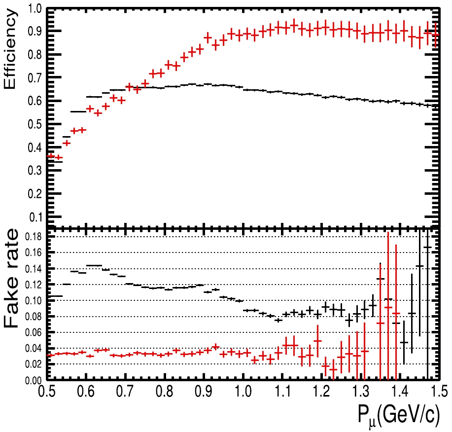
Figure 2. (color online) Detection efficiency of muon and the mis-identification rate of
$\pi/\mu$ for two efficiency curves provided by fast simulation.To suppress the background from
$ \tau^{-}\to K_{S}\pi^{-}(\geqslant 1 \pi^{0})\nu_{\tau} $ processes,$ \pi^{0} $ is reconstructed by selecting two good photons, and the event is rejected if the invariant mass of any two photons is located in the region between 0.12 and 0.15 GeV/$ c^{2} $ . The good photon candidates are selected with the efficiency sampled from fast simulation.After the above selection, the distribution of
$ K_{S}\pi^{-} $ mass spectrum from generic MC is shown in Fig. 3(a). There are huge backgrounds from other$ \tau $ decay channels in$ e^{+}e^{-}\to\tau^{+}\tau^{-} $ , excluding the signal process and the hadronic final states containing multiple$ \pi $ final states. The selection efficiency of the signal and the suppression rate of backgrounds with the above selection criteria are listed in Table 1.
Figure 3. (color online) Invariant mass spectra of
$K_{S}\pi^{-}$ with combined e-tag and$\mu$ -tag. (a) Distribution without detector optimization or likelihood requirement$y_{L}$ . (b) Distribution with likelihood requirement but no detector optimization. (c) Distribution with likelihood requirement and detector optimization. MC samples are normalized to 1 ab$^{-1}$ integrated luminosity.Process $\varepsilon_{\rm{raw} }(\%)$ 

$\varepsilon_{y_{L} }(\%)$ 

$\varepsilon_{y_{L}\&{\rm{optimization}}}(\%)$ 

$e^{+}e^{-}\to \tau^{+}\tau^{-}$ ,

$\tau^{+}\to l^{+}\nu_{l}\bar{\nu}_{\tau}, \tau^{-}\to K_{S}\pi^{-}\nu_{\tau}$ 

$22.80\pm0.02$ 

$22.22\pm0.02$ 

$32.82\pm0.02$ 

$e^{+}e^{-}\to \tau^{+}\tau^{-}$ (excluding signal process)

$0.182$ 

$0.0403$ 

$0.0422$ 

hadronic final states $0.304$ 

$0.0211$ 

$0.0179$ 

Table 1. Selection efficiencies for signal and background processes, with neither detector optimization nor likelihood requirement
$\varepsilon_{\rm{raw}}$ , with no detector optimization but applying likelihood requirement$\varepsilon_{{y_{L}}}$ , and with both detector optimization and likelihood requirement$\varepsilon_{{y_{L}}\&{\rm{optimization}}}$ . The errors are statistical only. For background processes, the statistical uncertainties are too small and can be neglected.To further suppress the background events, a likelihood ratio
$ y_{L} $ is used, defined by$ y_{L}(\vec{x}) = \frac{L_{S}(\vec{x})}{L_{S}(\vec{x})+L_{B}(\vec{x})}, $

(8) where
$ L_{S} $ and$ L_{B} $ are the likelihood functions for signal and background events, respectively.$ \vec{x} $ is a set of variables used for likelihood. Each likelihood function$ L_{S/B} $ is the product of the probability density function (PDF) of the input variables, defined by$ {L_{S/B}} = \prod\limits_{k = 1}^{{n_{var}}} {{P_{S/B,k}}} ({x_k}), $

(9) where
$ P_{S/B,k} $ is the signal/background PDF of the k-th input variable$ x_{k} $ . For this analysis, the set of variables$ \vec{x} $ includes the number of neutral clusters, momenta of decay products of$ K_{S} $ , decay length of$ K_{S} $ , mass spectrum of$ K_{S} $ ,$ \chi^{2} $ of$ K_{S} $ from secondary vertex fit,$ E/p $ ratio of the electron, momentum of$ \mu $ , cosine of the polar angle of$ \mu $ , and momenta of$ \pi $ and$ K_{S}\pi $ . The likelihood ratio$ y_{L}(\vec{x}) $ from these variables between signal and backgrounds is shown in Fig. 4, as well as the figure-of-merit. The classifier requirement on$ y_{L}(\vec{x}) $ is determined, by optimizing the figure-of-merit, to be 0.9979. The mass spectrum of$ K_{S}\pi^{-} $ after the above selections is shown in Fig. 3(b), and it is obvious that after likelihood requirements, the background level has been significantly suppressed. The selection efficiencies for signal and background processes with likelihood requirement are also shown in Table 1.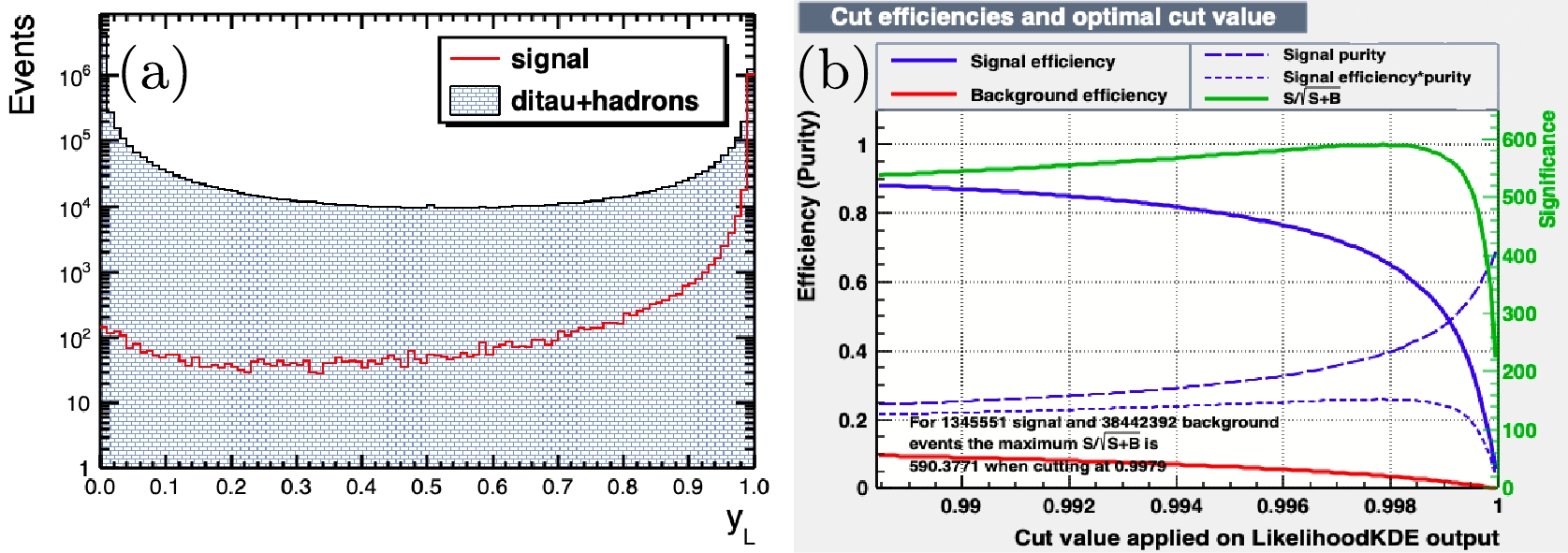
Figure 4. (color online) (a) Training and test sample distributions. The x-axis denotes
$y_{L}$ and the y-axis, which is set at log scale, denotes the entries. The signal is the process$\tau^{-}\to K_{S}\pi^{-}\nu_{\tau}$ . The backgrounds are$e^{+}e^{-}\to\tau^{+}\tau^{-}$ with$\tau$ decays excluding the signal processes and the hadronic final states. (b) The figure-of-merit for the likelihood selection. MC samples are normalized to 1 ab$^{-1}$ integrated luminosity.The background events surviving the above selection criteria come from hadronic final states or
$e^{+}e^{-}\to $ $ \tau^{+}\tau^{-}$ decay products, where$ e^{+}e^{-}\to\tau^{+}\tau^{-} $ is mainly from the final processes with one additional$ \pi^{0} $ , or multiple pion final states. At higher c.m. energies, the thrust T can be used to separate the hadronic final states from the signal process, defined as$ T\equiv \max\nolimits_{\overrightarrow{n}}\frac{\sum_i |\overrightarrow{\,n}\cdot\overrightarrow{p}_{i}|}{\sum_i |\overrightarrow{\,p}_{i}|}, $

(10) where
$ \overrightarrow{p}_{i} $ is the 3-momenta of the final state particles,$ \overrightarrow{n} $ is a 3-vector with unit norm. Finding$ \overrightarrow{n} $ in any direction of space makes the thrust T maximum. The typical distributions of thrust T at c.m. energy$ \sqrt{s} = 4.26 $ and 7.0 GeV are shown in Fig. 5 for both signal and hadronic processes. It is found that the thrust T can distinguish clearly between signal and hadronic background at high c.m. energies such as$ \sqrt{s} = 7.0 $ GeV. At lower c.m. energies, it is hard to distinguish the signal from background due to insufficient boost. However, with a good description of the hadronic final states from LUNDARLW, these backgrounds can be described well with MC simulation.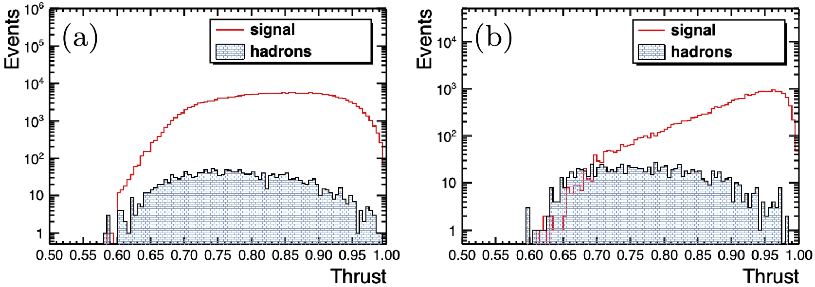
Figure 5. (color online) Distribution of thrust T (log scale in y-axis) at c.m.energy (a)
$\sqrt{s}=4.26$ GeV and (b)$\sqrt{s}=7.0$ GeV. The solid red line shows the signal process and the blue shaded area shows hadronic processes. MC samples are normalized to 1 ab$^{-1}$ integrated luminosity. -
After the above selection criteria, the signal process is selected with an efficiency of 22.22%, where the main loss of efficiency comes from the effects of track selection, reconstruction of
$ K_{S} $ , and particle identification of leptons. These effects correspond to the sub-detectors of the inner tracker, the PID system, and the MUD. By studying the signal-to-background ratios in the selection of the signal process with varying sub-detector responses, the requirements of detector design can be optimized accordingly. With the interfaces provided by fast simulation software, four kinds of detector response can be studied.a.Tracking efficiency The tracking efficiency in fast simulation is characterized by two dimensions: transverse momentum
$ P_{T} $ and polar angle$ \cos\theta $ , which are correlated with the level of track bending and the hit positions of tracks in the tracker system. For low-momentum tracks ($ P_{T}<0.2 $ GeV/c), it is difficult to reconstruct efficiently due to stronger electromagnetic multiple scattering, electric field leakage, energy loss, etc. However, with different techniques of inner tracker design at STCF, or with advanced track-finding algorithms, the reconstruction efficiency of low-momentum tracks can be improved.In this analysis, the efficiency is scaled in the fast simulation, with a ratio from 1 to 1.4 for low-momentum tracks, which indicates increasing the tracking efficiency by a factor of 10% to 40%. For high-momentum tracks or tracks with efficiency approximately 100%, the tracking efficiency remains the same. The figure-of-merit for each scale factor of low-momentum tracking efficiency is shown in Fig. 6, defined by
$ \dfrac{S}{\sqrt{S+B}} $ , where S denotes the signal yields of$ \tau^{-}\to K_{S}\pi^{-}\nu_{\tau} $ , and B denotes the backgrounds, both normalized to 1 ab$ ^{-1} $ integrated luminosity. From Fig. 6, it is found that the efficiency can be significantly improved with an optimization factor of 1.1 to 1.2.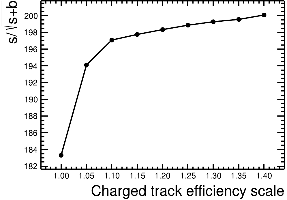
Figure 6. The figure-of-merit for optimization of the tracking efficiency for low-momentum tracks.
In fast simulation, the default tracking efficiency is sampled from the performance of the helium-gas-based cylindrical main drift chamber [50]. There are several alternative options for the tracker technique, especially for the inner tracker, such as a silicon pixel detector [57] or micro-pattern gaseous detector [58]. From the current R&D activities, the tracking efficiency for low-momentum tracks is expected to fulfill the request from our analysis of these techniques at STCF.
b. Momentum/spatial resolution The momentum and spatial resolution can also be optimized in fast simulation with proper scaling factors. A better resolution will improve the significance of signal with the improvement of resolution in the
$ K_{S}\pi^{-} $ mass spectrum. The effects of momentum and position resolutions on$ K_{S} $ reconstruction efficiency are also studied, and it is found that the spatial resolution is more sensitive than the momentum resolution for$ K_{S} $ reconstruction. From the reconstruction method for a charged track, these two resolutions are related to the same sources, which are the position resolution of a single wire in the$ xy $ plane and z direction, and multiple scattering. Micro-pattern gaseous detectors can achieve excellent position accuracy [58]. Besides, a MC study on the silicon pixel detector shows that the momentum resolution and tracking efficiency can be significantly improved due to its good spatial resolution [59].c.
$ \pi/\mu $ separation As discussed before, there are two efficiency curves provided for$ \mu $ identification. The default muon identification in the fast simulation has a large$ \pi/\mu $ mis-identification rate, as shown by the black points in Fig. 2. As the fast simulation provides a function for optimizing the$ \pi/\mu $ mis-identification, we can vary the mis-identification rate for$ \pi/\mu $ based on the provided efficiency curves. The signal-to-background ratio can be significantly improved with a better$ \pi/\mu $ mid-identification rate. The$ \pi/\mu $ separation power can also be significantly improved with a hybrid design for MUD [50], and the efficiency curves are shown by the red points in Fig. 2 for the requirement of$ \pi/\mu $ mis-identification to be 3%. Three mis-identification rates are provided for the MUD, with different efficiencies for$ \mu $ . Table 2 summarizes the selection efficiency for these three efficiency responses. The detector efficiency for the signal process is highest for the$ \pi/\mu $ mis-identification at 3%, because a moderate selection on the performance of the MUD is applied with this requirement. Moreover, at STCF, the Ring Imaging CHerenkov detector (RICH) can be used to identify muons from pions at low momentum.FR(%) Eff. $\mu$ (%)

Eff. bkg(%) Final eff.(%) 3 $76.80\pm0.02$ 

0.385 $32.82\pm0.02$ 

1.7 $66.79\pm0.02$ 

0.375 $31.40\pm0.02$ 

1 $58.63\pm0.03$ 

0.370 $30.20\pm0.02$ 

Table 2. Efficiency of selecting
$\mu$ and final selection efficiency using a hybrid design for MUD at STCF with different$\pi/\mu$ fake rate (FR) requirements.d. Position/energy resolution for photons. In this analysis, processes including
$ \pi^{0} $ are suppressed by vetoing events with a reconstructed$ \pi^{0} $ . The position and energy resolutions for neutral tracks are optimized with the fast simulation. It is found that the current resolutions provided in the fast simulation, 6 mm for position resolution and 2.5% for energy resolution of a 1 GeV photon, can satisfy the physical requirements for this analysis.From the above study, a set of optimization factors for sub-detector responses for this analysis is provided: an improvement of tracking efficiency by a factor of
$10\% \sim 20\%$ for low-momentum tracks; a good momentum/spatial resolution for charged tracks; a good muon identification with the mis-identification rate of$ \pi/\mu $ to be less than 3%; and a good position/energy resolution for photons. With these optimization factors applied, the selection efficiency for signal process is improved from 22.22% to 32.82%. The invariant mass of$ K_{S}\pi^{-} $ after optimization is shown in Fig. 3(c). The background level is significantly suppressed, where the dominant$ \tau $ pair decay background events are$ \tau^{-}\to\pi^{+}\pi^{-}\pi^{-}\nu_{\tau} $ and$ \tau^{-}\to K_{S}\pi^{-}\pi^{0}\nu_{\tau} $ . The optimized selection efficiency and the background levels are summarized in Table 1. The detailed selection efficiencies for each step are listed in Table 3, where the improvement of the selection efficiency compared to the MC without optimization is given.Selection $\varepsilon$ (%)

$\varepsilon_{\rm{rela}}$ (%)

$\Delta\varepsilon_{\rm{rela}}$ (%)

$N_{\rm{charged\_track}}$ 

$69.75\pm0.02$ 

$69.75$ 

7.52 select $K_{S}$ 

$54.34\pm0.03$ 

$77.90$ 

$13.10$ 

lepton ID $37.89\pm0.03$ 

$87.31$ 

19.13 $\pi$ ID

$36.64\pm0.03$ 

$96.70$ 

2.66 veto $\pi^{0}$ 

$36.64\pm0.03$ 

$99.99$ 

− $K_{S}$ flight length

$33.45\pm0.02$ 

$91.38$ 

0.27 likelihood method $32.82\pm0.02$ 

$98.10$ 

0.52 Total $32.82\pm0.02$ 

$-$ 

$ -$ 

Table 3. Cut flow for each selection criterion for the signal process, where
$\varepsilon$ is the overall efficiency,$\varepsilon_{\rm{rela}}$ is the relative efficiency for each criterion, and$\Delta\varepsilon_{\rm{rela}}$ is the relative improvement of optimized detector response compared to the original. -
With the above selection criteria and optimization procedure, the numbers of signal events from
$ \tau^{-} $ and$ \tau^{+} $ decays with generic MC normalized to 1 ab$ ^{-1} $ integrated luminosity are obtained by fitting the$ K_{S}\pi $ invariant mass with the RooFit tool, where the signal can be parameterized by the function shown in Eq. (4) and the background is described with simulated background. The efficiency-corrected numbers for$ \tau^{-}\to K_{S}\pi^{-}\nu_{\tau} $ and$ \tau^{+}\to K_{S}\pi^{+}\bar{\nu}_{\tau} $ are$ 3681017\pm5034 $ and$ 3681127\pm5091 $ , respectively. This shows a good consistency with the input values. The statistical sensitivity of CPV with decay rate can be calculated, using Eq. (1), to be$ 9.7\times10^{-4} $ . Since the cross-section of$ e^{+}e^{-}\to\tau^{+}\tau^{-} $ is around 3.5 nb in the energy region from$ \sqrt{s} = 4.0 $ to 5.0 GeV, we studied the selection efficiency for the signal process in this energy region, as shown in Fig. 7. The efficiencies in this energy region vary from 32.82% to 32.03%, with a relative difference of less than 3%. Therefore, the statistics of the signal process increase linearly with more data collected. As the event selection is not background-free, the sensitivity of CPV is proportional to$ 1/\sqrt{L} $ , as shown in Fig. 7(b), where different sizes of MC samples, from 0.1 ab$ ^{-1} $ to 1.0 ab$ ^{-1} $ are applied for the study. Finally, we can conclude that, with 10 ab$ ^{-1} $ integrated luminosity collected at STCF from$ \sqrt{s} = 4.0 $ to 5.0 GeV, the sensitivity of CPV for the process$ \tau^{-}\to K_{S}\pi^{-}\nu_{\tau} $ is$ 3.1\times10^{-4} $ .
Figure 7. (a) Selection efficiencies for the signal process at different c.m. energies from
$\sqrt{s}=4.0$ GeV to 5.0 GeV. (b) CPV sensitivity of$\tau^{-}\to K_{S}\pi^{-}\nu_{\tau}$ for varying integrated luminosity L, following$1/\sqrt{L}$ extrapolation.Though this analysis is performed purely with MC simulation, we need to discuss possible systematic uncertainties which may bias the decay-rate asymmetry measurement between
$ \tau^{-}\to K_{S}\pi^{-}\nu_{\tau} $ and$ \tau^{+}\to K_{S}\pi^{+}\bar{\nu}_{\tau} $ . The sources of uncertainty are estimated as follows. i) The detection asymmetry for charged particles, which can be studied from a control sample of$ \tau^{-}\to \pi^{+}\pi^{-}\pi^{-}\nu_{\tau} $ . The difference from the detector can be corrected by comparing the asymmetry between MC simulation and data, and the remaining uncertainty is related to the statistical uncertainty of the control sample. Since the branching fraction of the control sample is over one order of magnitude larger than the signal process, the uncertainty will be significantly smaller than the statistical uncertainty of$ \tau^{-}\to K_{S}\pi^{-}\nu_{\tau} $ . ii) Uncertainty related to the selection criteria, which can be studied by varying the selection criteria. By performing the Barlow test [60], any bias from selection will be studied and corrected until the systematic accuracy matches the statistical precision. iii) Uncertainty from the MC generator. In this analysis, no CPV is modeled and the output asymmetry in MC is about$ 3\times10^{-5} $ , which can be neglected. iv) Uncertainty from background contamination. In this analysis, there is no decay-rate asymmetry observed in the background, and the uncertainty can be tested by applying different criteria to the background between data and MC simulation. v) The different nuclear-interaction cross sections of the$ K^{0} $ and$ \bar{K}^{0} $ meson. In Ref. [28], a correction to the asymmetry accounting from$ K^{0} $ and$ \bar{K}^{0} $ mesons with material in the detector was applied by taking the$ K^{\pm} $ nucleon cross-sections as an analogy under the assumption of isospin invariance [61]. We take an uncertainty of 0.01% for this uncertainty, similar to that from Ref. [28], ignoring the material difference at STCF. As a consequence of the above discussion, the systematic uncertainty for a decay-rate asymmetry study of$ \tau^{-}\to K_{S}\pi^{-}\nu_{\tau} $ will be at the same level as its statistical uncertainty.As introduced before, the sensitivity of CPV in the processes of
$ \tau^{-}\to K_{S}\pi^{-}\nu_{\tau} $ at the Belle II experiment is expected to be$ 1/\sqrt{70} $ of the current precision of the Belle experiment with a 50 ab$ ^{-1} $ data sample collected [43], which is better than the sensitivity obtained at STCF with one year of data taking, but comparable with that at STCF with ten years of data taking. The study of$ \tau^{-}\to K_{S}\pi^{-}\nu_{\tau} $ at a B-factory benefits from a larger luminosity, and a good separation of the two hemispheres from$ \tau^{+} $ and$ \tau^{-} $ decay. However, at STCF, the cross section of$ e^{+}e^{-}\to\tau^{+}\tau^{-} $ is the largest and the selection efficiency for the signal process is better with high detection/PID efficiency for low-momentum tracks. When the c.m. energy goes up, e.g. at$ \sqrt{s} = 7 $ GeV, the two hemispheres from$ \tau^{+} $ and$ \tau^{-} $ decays can also be separated well, as shown in Fig. 5. Therefore, it is of great potential to study the CPV and relevant physics program of the process$ \tau^{-}\to K_{S}\pi^{-}\nu_{\tau} $ at STCF. -
In this paper, the sensitivity of the decay-rate asymmetry in
$ \tau^{-}\to K_{S}\pi^{-}\nu_{\tau} $ decays is studied at$ \sqrt{s} = 4.26 $ GeV with 1 ab$ ^{-1} $ inclusive MC. Benefitting from the largest cross-section of 3.5 nb for$ e^{+}e^{-}\to\tau^{+}\tau^{-} $ at$ \sqrt{s} = 4.26 $ GeV, and the optimized efficiency with the fast simulation, the statistical sensitivity of CPV is$ 9.7\times10^{-4} $ , which is 2.3 times better than that of BaBar [28]. With 10 ab$ ^{-1} $ luminosity collected at STCF, the sensitivity is expected to be at a level of$ 3.1\times10^{-4} $ , which is comparable to the uncertainty of theoretical prediction in the SM. A new round of measurements of$ A_{CP} $ defined by the decay rate difference is important and desirable, c.f. Eq. (2), and will certainly shed light on the existence of the NP signal. Several theoretical models discussed in Sec. II will be reexamined. CPV in the exchange of charged Higgs bosons has also been explored in experiments, and is defined by the difference between angular observables, as a helpful complement. With this precision of$ 10^{-4} $ , re-measurement of this channel will be pursued. Meanwhile, the other prospects mentioned (form factors,$ |V_{us}| $ extraction etc.) could be examined. -
The authors thank the USTC Supercomputing Center and the Hefei Comprehensive National Science Center for their strong support.
Feasibility study of CP violation in ${{{\mathit{\boldsymbol{\tau^-}}}} {\mathit{\boldsymbol{\rightarrow K_{S}}}\pi^{-} \nu_{\tau}}}$ decays at the Super Tau Charm Facility
- Received Date: 2020-12-15
- Available Online: 2021-05-15
Abstract: We report a feasibility study for violation in


 DownLoad: