


 Abstract
 HTML
HTML Reference
 Related
 PDF
PDF


-
The Schwinger pair production of charged particles is an important QED phenomenon that is related to the vacuum instability and persistence in the presence of strong external electromagnetic fields [1]. Another important spontaneous pair production phenomenon is the Hawking radiation from black holes, which can be viewed as a tunneling process through the black hole horizon [2]. A charged black hole thus provides a natural lab in which both the Schwinger pair production and the Hawking radiation can occur and mix with each other. Usually the equation of motions (EoMs) of quantum fields in a general black hole background is difficult to solve analytically in full spacetime. However, when the symmetry of the spacetime geometry is enhanced under some conditions, the problem becomes manageable; for this reason, in a series of recent studies, the spontaneous pair production of charged particles has been systematically studied in near extremal charged black holes, including the RN black hole [3-5] and the Kerr-Newman (KN) black hole [6, 7], in which the near horizon geometry is enhanced into AdS2 or warped AdS3 in the near extremal limit. Owing to the enhanced near horizon symmetry, the explicit forms of the pair production rate and other 2-point correlation functions have been obtained and their holographic descriptions have been found based on the RN/CFT [8-13] and KN/CFTs dualities [14-16]. In addition to charged black hole backgrounds, pair production has also been investigated in pure AdS or dS spacetime, see, e.g., [17-20], whereas in the absence of a gravitational field, the pure Schwinger effect has been efficiently analyzed by using the phase-integral method [21-24].
However, previous studies mainly focused on analyzing spontaneous pair production in the near horizon region of black holes in an asymptotically flat spacetime. A charged black hole in AdS spacetime has an additional AdS symmetry at the asymptotical boundary. From the holographic point of view, the CFT description of pair production has been revealed only in the near horizon region in terms of AdS2/CFT1 (or warped AdS3/CFT2). Although particle pairs produced in the near horizon region of black holes indeed provide important contributions to those in full spacetime, an understanding of the whole picture is still lacking. In the present paper, we extend the study of pair production to a full near extremal RN-AdS5 black hole background, which possesses an AdS5 geometry at the asymptotic spatial boundary as well as an AdS2 structure in the near horizon region. It is shown that the radial equation of the charged scalar field propagating in this spacetime can be transformed into a Heun-like differential equation and thus be solved by matching its solutions in the near and far spacetime regions, using the low temperature limit. Consequently, analytical forms of the full solutions for the pair production rate, the absorption cross section ratio, and the retarded Green's functions are obtained, and they are shown to have concise relations with their counterparts calculated in the near horizon region. Based on these concise relations, numerical analysis can easily be performed, and the pair production rate in full spacetime is shown to be smaller than that in the near horizon region, which is consistent with the assumption that pair production mainly comes from the black hole near horizon region.
A near extremal RN-AdS5 black hole is also a very useful background for studying holographic dualities. As the near horizon AdS2 (or warped AdS3) spacetime is dual to a 1D CFT (or chiral CFT2), while asymptotical AdS5 spacetime is dual to another 4D CFT, the former is called IR CFT, while the latter is called UV CFT, and they are connected with each other via the holographic renormalization group (RG) flow along the radial direction [25-27]. For example, it has been shown that a near extremal RN-AdS black hole acts as a holographic model in describing typical properties of a (non)Fermi liquid at the quantum critical point [28-31]. It is thus natural and interesting to find holographic descriptions of pair production in an RN-AdS5 black hole both in the IR CFT1 in the near horizon region and the UV CFT4 at the asymptotical AdS5 boundary. We show that the picture in the IR CFT1 is very similar to those in the near extremal RN and KN black holes, and that the pair production rate and the absorption cross section ratio calculated from the AdS2 spacetime can be matched with those from the dual IR CFT. Regarding the UV 4D CFT, a direct comparison of calculations between the bulk and the boundary in terms of the AdS5/CFT4 is not made due to a lack of information on the dual finite temperature CFT4 side. However, from the bulk gravity side, the condition for pair production in the full near extremal RN-AdS5 spacetime is the violation of the Breitenlohner-Freedman (BF) bound [32, 33] in AdS5 spacetime. This, on the dual 4D CFT side, corresponds to a complex conformal weight for the scalar operator dual to the bulk charged scalar field, which indeed indicates instabilities for the scalar operator on the boundary and is consistent with the situation in the IR CFT. Furthermore, we determined an interesting relation between the full pair production rate and the absorption cross section ratio via changing the roles of sources and operators simultaneously both in the IR and the UV CFTs.
The rest of the paper is organized as follows. In Sec. II, we provide a brief review of the bulk theory and consider the near horizon geometry of an RN-
$ {\rm{AdS}}_{d+1} $ black hole and the EoMs of the probe charged scalar field. In Sec. III, spontaneous pair production in the near horizon region of near extremal RN-$ {\rm{AdS}}_{d+1} $ black holes is discussed, and the 2-point functions of the charged scalar field (such as the retarded Green's function), pair production rate, and absorption cross section ratio are calculated. In Sec. IV, the full analytical solution for the radial equation of the charged scalar field in RN-AdS5 black holes is obtained by applying the matching technique. Consequently, the full analytical forms of the pair production rate, absorption cross section ratio, and retarded Green's function are found, and the connections with their counterparts in the near horizon region of the black hole are discussed. Then, in Sec. V, the dual CFTs descriptions of spontaneous pair production are both analyzed in terms of the AdS2/CFT1 correspondence in the IR region and the AdS5/CFT4 correspondence in the UV region, and their connections are also revealed. Finally, the conclusion and physical implications are provided in Sec. VI. -
The
$ d+1 $ dimensional Einstein-Maxwell theory has an action (in units of$ c = \hbar = 1 $ ) as$ I = \int {\rm d}^{d+1}x \sqrt{-g} \left[ \frac{1}{16 \pi G_{d+1}} \left( R + \frac{d(d-1)}{L^2} \right) - \frac1{g_{\mathrm s}^2} F_{\mu\nu} F^{\mu\nu} \right], $

(1) where L is the curvature radius of the asymptotical
$ {\rm{AdS}}_{d+1} $ spacetime, and$ g_{\mathrm s} $ is the dimensionless coupling constant of the$ U(1) $ gauge field. The dynamical equations$ \begin{aligned}[b] R_{\mu\nu} \!-\! \frac12 g_{\mu\nu} R \!-\! \frac{d(d-1)}{2L^2} g_{\mu\nu} & \!=\! \frac{8 \pi G_{d+1}}{g_{\mathrm s}^2} \left( 4 F_{\mu\lambda} F_{\nu}{}^{\lambda} \!-\! g_{\mu\nu} F_{\alpha\beta} F^{\alpha\beta} \right), \\ \partial_\mu \left( \sqrt{-g} F^{\mu\nu} \right) & = 0, \end{aligned} $

(2) admit the Reissner-Nordström-Anti de Sitter (RN-
$ {\rm{AdS}}_{d+1} $ ) black brane (or the planar black hole) solution [34]$ \begin{aligned}[b] {\rm d}s^2 & = \frac{L^2}{r^2 f(r)} {\rm d}r^2 + \frac{r^2}{L^2} \left( -f(r) {\rm d}t^2 + {\rm d}x_i^2 \right), \\ A & = \mu \left( 1 - \dfrac{r_{\mathrm o}^{d-2}}{r^{d-2}} \right) {\rm d}t, \end{aligned} $

(3) with
$\begin{aligned}[b] f(r) =& 1 - \frac{G_{d+1} L^2 M}{r^d} + \frac{G_{d+1} L^2 Q^2}{r^{2d-2}}, \qquad {} \\ \mu =& \sqrt{\frac{d-1}{2(d-2)}} \frac{g_{\mathrm s} Q}{r_{\mathrm o}^{d-2}},\end{aligned} $

(4) where
$ r_{\mathrm o} $ is the radius of the outer horizon ($ f(r_{\mathrm o}) = 0 $ ),$ \mu $ is the chemical potential with dimension$ [\mu] = \mathrm{length}^{-(d-1)/2} $ , M is the mass, and Q is the charge of the black brane. We may find an explicit expression of$ r_{\mathrm o} $ for$ d = 4 $ from a solution of the cubic equation, which is complicated, but$ r_\mathrm{o} $ has a general expression in the extremal case, i.e.,$ r_* $ in IIB. The condition$ f(r_{\mathrm o}) = 0 $ gives$ M = \dfrac{r_{\mathrm o}^d}{G_{d+1} L^2} + \dfrac{Q^2}{r_{\mathrm o}^{d-2}} $ (which is the Smarr-like relation related to the first law of thermodynamics of the black brane); temperature T and “surface” entropy density s of the black brane are, respectively,$\begin{aligned}[b] T =& \frac{r_{\mathrm o} \, d}{4\pi L^2} \left( 1 - \frac{d-2}{d} \frac{G_{d+1} L^2 Q^2}{r_{\mathrm o}^{2d-2}} \right), \qquad {\rm{}} \\ s = &\frac{1}{4G_{d+1}} \left( \frac{r_{\mathrm o}}{L} \right)^{d-1}. \end{aligned} $

(5) Moreover, the first law of thermodynamics of the dual boundary d-dimensional quantum field is
$ \delta \epsilon = T \delta s + \mu \delta\rho_{\mathrm c}, $

(6) where the “surface” energy and charge densities are, respectively,
$ \begin{aligned}[b]& \epsilon = \frac{d - 1}{16 \pi L^{d-1}} M, \qquad {\rm{}} \qquad \\&\rho_{\mathrm c} = \frac{\sqrt{2(d-1)(d-2)}}{8 \pi g_{\mathrm s} L^{d-1}} Q. \end{aligned} $

(7) Then, it is straightforward to check the Euler relation
$ \left( \frac{d}{d-1} \right) \epsilon = \epsilon + p = T s + \mu \rho_{\mathrm c}, $

(8) where the pressure is
$ p = \dfrac{\epsilon}{d-1} $ , which shows that the dual d-dimensional quantum field theory on the asymptotic boundary is conformal, as expected. -
To make the following analysis convenient, let us introduce the length scale
$ r_*^{2d-2} \equiv \dfrac{d-2}{d} G_{d+1} L^2 Q^2 $ ; then, the temperature can be rewritten as$ T = \frac{r_{\mathrm o} d}{4\pi L^2} \left( 1 - \frac{r_*^{2d-2}}{r_{\mathrm o}^{2d-2}} \right). $

(9) Note that
$ r_* $ may be treated as the “effective” radius of the inner black hole horizon though$ f(r_*) \neq 0 $ in general and$ r_* < r_{\mathrm o} $ . The extremal condition for a degenerate horizon at$ r_\mathrm{o} = r_* $ is$ M = M_0 \equiv \dfrac{2 (d-1)}{d-2} \dfrac{r_*^d}{G_{d+1} L^2} $ . The near extremal limit of the near horizon is obtained by taking the limit$ \varepsilon \to 0 $ of the transformations$ \begin{aligned}[b]& M - M_0 = \frac{d (d-1) r_*^{d-2}}{G_{d+1} L^2} \varepsilon^2 \rho_\mathrm{o}^2, \\& r_{\mathrm o} - r_* = \varepsilon \rho_{\mathrm o}, \quad r - r_{\mathrm o} = \varepsilon (\rho - \rho_0), \quad t = \frac{\tau}{\varepsilon}, \end{aligned}$

(10) where in general
$ \rho_{\mathrm o} $ is finite and$ \rho \in [\rho_0, \infty) $ .Expanding
$ f(r) $ around$ r = r_{\mathrm o} $ , we have$ f(r) \simeq \frac{{d(d - 1)}}{{r_{\rm{o}}^2}}({\rho ^2} - \rho _{\rm{o}}^2){\varepsilon ^2} + O\left( {{\varepsilon ^3}} \right), $

(11) the near horizon geometry is given by
$ \begin{aligned}[b] {\rm d}s^2 & = - \frac{\rho^2 - \rho_{\mathrm o}^2}{\ell^2} {\rm d}\tau^2 + \frac{\ell^2 {\rm d}\rho^2}{\rho^2 - \rho_{\mathrm o}^2} + \frac{r_{\mathrm o}^2}{L^2} {\rm d}x_i^2, \\ A & = \frac{(d-2) \mu}{r_{\mathrm o}} (\rho - \rho_{\mathrm o}) {\rm d}\tau, \end{aligned} $

(12) where
$ \ell^2 \equiv \dfrac{L^2}{d (d - 1)} $ is defined as the square of the curvature radius of the effective AdS2 geometry. The limit$ \rho_{\mathrm o} \to 0 $ yields the extremal limit.The solution in Eq. (12) can also be written in the Poincaré coordinates in terms of
$ \xi = \ell^2/\rho $ , ($ |\xi| \leqslant \xi_{\mathrm o} = $ $ \ell^2/\rho_\mathrm{o} $ ),$ \begin{aligned}[b] {\rm d}s^2 & = \frac{\ell^2}{\xi^2} \left( - \left( 1 - \frac{\xi^2}{\xi_{\mathrm o}^2} \right) {\rm d}\tau^2 + \frac{{\rm d}\xi^2}{1-\dfrac{\xi^2}{\xi_{\mathrm o}^2}} \right) + \frac{r_{\mathrm o}^2}{L^2} {\rm d}x_i^2, \\ A & = \frac{(d-2) \mu \ell^2}{r_{\mathrm o}} \left( \frac{1}{\xi} - \frac{1}{\xi_{\mathrm o}} \right) {\rm d}\tau. \end{aligned} $

(13) The above geometry is a black brane with both local and asymptotical topology
$ {\rm{AdS}}_2 \times {{R}}^{d-1} $ (AdS2 has the$ SL(2,R)_R $ symmetry). The horizons of the new black brane are located at$ \xi = \pm \xi_{\mathrm o} $ , and its temperature is$ T_{ {{n}}} = \dfrac{1}{2 \pi \xi_{\mathrm o}} $ . Note that if we adopt the new coordinates$ z \equiv \xi/\xi_{\mathrm o} $ with$ |z| \leqslant 1 $ and$ \eta = \tau/\xi_{\mathrm o} $ , the metric becomes$ {\rm d}s^2 = \frac{\ell^2}{z^2} \left( - (1 - z^2) {\rm d}\eta^2 + \frac{{\rm d}z^2}{1-z^2} \right) + \frac{r_{\mathrm o}^2}{L^2} {\rm d}x_i^2, $

(14) and the temperature associated with the inverse period of
$ \eta $ is normalized to$ \tilde{T}_{ n} = \dfrac{1}{2\pi} $ . -
The action of a bulk probe charged scalar field
$ \Phi $ with mass m and charge q is$ S = \int {{{\rm d}^{d + 1}}} x\sqrt { - g} \left( { - \frac{1}{2}{D_\alpha^* }{\Phi ^*}{D^\alpha }\Phi - \frac{1}{2}{m^2}{\Phi ^*}\Phi } \right), $

(15) where
$ D_{\alpha} \equiv \nabla_{\alpha} - {\rm i} q A_{\alpha} $ with$ \nabla_\alpha $ being the covariant derivative in curved spacetime. The corresponding Klein-Gordon (KG) equation is$ (\nabla_\alpha - {\rm i} q A_\alpha) (\nabla^\alpha - {\rm i} q A^\alpha) \Phi = m^2 \Phi. $

(16) Moreover, the radial flux of the probe field is
$ {\cal F} = {\rm i}\sqrt { - g} {g^{rr}}(\Phi D_r^*{\Phi ^*} - {\Phi ^*}{D_r}\Phi ). $

(17) In the RN-
$ {\rm{AdS}}_{d+1} $ background (3), assuming$ \Phi(t, \vec{x}, r) = $ $ \phi(r) \mathrm{e}^{-{\rm i} \omega t + {\rm i} \vec{k} \cdot \vec{x}} $ , the KG Eq. (16) has the radial form$ \begin{aligned}[b]& \left(\frac{L}{r}\right)^{d-1} \partial_r \left( \frac{r^{d+1}}{L^{d+1}} f(r) \partial_r \right) \phi(r) \\& + \left(\frac{L^2 (\omega + q A_t)^2}{r^2 f(r)} - m^2 - \frac{L^2}{r^2} \vec{k}^2 \right) \phi(r) = 0. \end{aligned}$

(18) The solutions to Eq. (18) cannot be directly found in terms of special functions in the full spacetime region. In what follows, we solve it in different regions and match these solutions to obtain the full solution.
-
Firstly, we analyze the near horizon, near extreme region (13) and solve the KG Eq. (16) by expanding the scalar field as
$ \Phi(\tau, \vec{x}, \xi) = \phi(\xi) \mathrm{e}^{-{\rm i} w \tau + {\rm i} \vec{k} \cdot \vec{x}}. $

(19) Then, the KG equation reduces to ①
$\begin{aligned}[b] \xi^2 \left( 1 - \frac{\xi^2}{\xi_{\mathrm o}^2} \right) \phi''(\xi) - \frac{2\xi^3}{\xi_{\mathrm o}^2} \phi'(\xi) + \xi^2 \frac{(w + q A_\tau)^2}{1 - \dfrac{\xi^2}{\xi_{\mathrm o}^2}} \phi(\xi) = m_\mathrm{eff}^2 \ell^2 \phi(\xi), \end{aligned} $

(20) where the effective mass square is defined as
$ m_\mathrm{eff}^2 = $ $ m^2 + \dfrac{L^2 \vec{k}^2}{r_{\mathrm o}^2} $ , or the KG equation can be expressed in the z coordinate as$ \begin{aligned}[b] z^2 (1 - z^2) \phi''(z) - 2 z^3 \phi'(z) &+ \frac{z^2}{1 - z^2} \left[ \left( w \xi_{\mathrm o} + q_\mathrm{eff} \ell \frac{1 - z}{z} \right)^2\right. \\&\left.- m_\mathrm{eff}^2 \ell^2 \frac{1 - z^2}{z^2} \right] \phi(z) = 0, \end{aligned} $

(21) where the effective charge of the probe field is
$ q_\mathrm{eff} \equiv $ $ (d-2) \dfrac{\mu \ell}{r_{\mathrm o}} q $ . The singularities of Eq. (21) are located at$ z = 0, z = \pm 1 $ and$ z = \infty $ .To find the solutions, we determine the indices at each singular point. For
$ z \to 0 $ , setting$ \phi(z) \sim z^{\bar{\alpha}} $ , the leading terms in Eq. (21) are$ z^2 \phi''(z) + (q_\mathrm{eff}^2 - m_\mathrm{eff}^2) \ell^2 \phi(z) = 0, $

(22) which gives
$ \begin{aligned}[b] \bar{\alpha} = &\frac12 \pm \frac12 \sqrt{1 + 4 ( m_\mathrm{eff}^2 - q_\mathrm{eff}^2 ) \ell^2} \\\equiv &\frac12 \pm \frac12 \sqrt{1 + 4 \tilde{m}_\mathrm{eff}^2 \ell^2} \equiv \frac12 \pm \nu. \end{aligned} $

(23) For
$ z \to -1 $ , setting$ \phi(z) \sim (1 + z)^{\bar{\beta}} $ , Eq. (21) reduces to$ 2 (1 + z) \phi''(z) + 2 \phi'(z) + \frac{(w \xi_{\mathrm o} - 2 q_\mathrm{eff} \ell)^2}{2 (1 + z)} \phi(z) = 0, $

(24) and the index is
$ \bar{\beta} = \pm {\rm i} \left( \frac{w \xi_{\mathrm o}}{2} - q_\mathrm{eff} \ell \right) = \pm {\rm i} \left( \frac{w}{4 \pi T_{\mathrm n}} - q_\mathrm{eff} \ell \right). $

(25) Finally, for
$ z \to 1 $ , setting$ \phi(z) \sim (1 - z)^{\bar{\gamma}} $ , Eq. (21) reduces to$ 2 (1 - z) \phi''(z) - 2 \phi'(z) + \frac{(w \xi_{\mathrm o})^2}{2 (1 - z)} \phi(z) = 0, $

(26) from which
$ \bar{\gamma} = \pm {\rm i} \frac{w \xi_{\mathrm o}}{2} = \pm {\rm i} \frac{w}{4 \pi T_{\mathrm n}} = \pm {\rm i}\frac{\omega/\varepsilon}{4\pi /(2\pi \xi_{\mathrm o})} = \pm {\rm i}\frac{\omega}{2\varepsilon\rho_{\mathrm o}/\ell^2} = \pm {\rm i}\frac{\omega}{4\pi T} $

(27) is obtained. Further, imposing the ingoing boundary condition at the black brane horizon
$ z = 1 $ requires$ \bar{\gamma} = $ $ -{\rm i} \dfrac{w \xi_{\mathrm o}}{2} = -{\rm i} \dfrac{w}{4\pi T_{\mathrm n}} $ .Also, note that Eq. (21) can be rewritten in a more explicit form as
$ \begin{aligned}[b] \phi''(z) + \left( \frac{1}{z+1} + \frac{1}{z-1} \right) \phi'(z) + \left( \frac{\tilde{m}_\mathrm{eff}^2 \ell^2}{z} + \frac{\dfrac{1}{2} (w \xi_{\mathrm o} - 2 q_\mathrm{eff} \ell)^2}{z+1} + \frac{\dfrac12 w^2 \xi_{\mathrm o}^2}{z-1} \right) \frac{\phi(z)}{z (z+1) (z-1)} = 0, \end{aligned} $ 
(28) which becomes the Fuchs equation with three canonical singularities
$ a_1 $ ,$ a_2 $ and$ a_3 $ , as follows:$ \begin{aligned}[b] \phi''(z) &+ \left( \frac{1-\bar{\alpha}_1-\bar{\alpha}_2}{z-a_1} + \frac{1-\bar{\beta}_1-\bar{\beta}_2}{z-a_2} + \frac{1-\bar{\gamma}_1-\bar{\gamma}_2}{z-a_3} \right) \phi'(z) + \left( \frac{\bar{\alpha}_1 \bar{\alpha}_2 (a_1-a_2) (a_1-a_3)}{z-a_1} + \frac{\bar{\beta}_1 \bar{\beta}_2 (a_2-a_3) (a_2-a_1)}{z-a_2}\right. \\&\left.+ \frac{\bar{\gamma}_1 \bar{\gamma}_2 (a_3-a_1) (a_3-a_2)}{z-a_3} \right) \frac{\phi(z)}{(z-a_1)(z-a_2)(z-a_3)} = 0, \end{aligned} $

(29) where
$ a_1 = 0 $ ,$ a_2 = -1 $ , and$ a_3 = 1 $ and$ \begin{aligned}[b]& \bar{\alpha}_1 = \frac12 \pm \nu, \quad \bar{\alpha}_2 = \frac12 \mp \nu, \quad \bar{\beta}_1 = - \bar{\beta}_2 = \pm {\rm i} \frac{w \xi_{\mathrm o} - 2 q_\mathrm{eff} \ell}2, \\& \bar{\gamma}_1 = - \bar{\gamma}_2 = \pm {\rm i} \frac{w \xi_{\mathrm o}}2, \end{aligned}$

(30) and
$ \bar{\alpha}_1 + \bar{\alpha}_2 + \bar{\beta}_1 + \bar{\beta}_2 + \bar{\gamma}_1 + \bar{\gamma}_2 = 1 $ is satisfied. The Fuchs Eq. (29) can be transformed into the standard hypergeometric function$ \zeta (1 - \zeta) \psi''(\zeta) + \left[ \tilde{\gamma} - (1 + \tilde{\alpha} + \tilde{\beta}) \zeta \right] \psi'(\zeta) - \tilde{\alpha} \tilde{\beta} \psi(\zeta) = 0, $

(31) via the conformal coordinate transformation
$ \zeta = \frac{(a_2-a_3)(z-a_1)}{(a_2-a_1)(z-a_3)}, \quad {\rm{}} \;\; \phi(z) = \left(\frac{z-a_1}{z-a_3}\right)^{\bar{\alpha}_1} \left(\frac{z-a_2}{z-a_3}\right)^{\bar{\beta}_1} \psi(\zeta), $

(32) where
$ \tilde{\alpha} = \bar{\alpha}_1 + \bar{\beta}_1 + \bar{\gamma}_1, \tilde{\beta} = \bar{\alpha}_1 + \bar{\beta}_1 + \bar{\gamma}_2 $ and$ \tilde{\gamma} = 1 + \bar{\alpha}_1 - \bar{\alpha}_2 $ . (Note that one can freely choose the indices$ i = 1,\; 2 $ for$ \bar{\alpha}_i $ ,$ \bar{\beta}_i $ and$ \bar{\gamma}_i $ .)For Eq. (28), we have
$ \zeta = 2z/(z-1) $ ,$\tilde{\alpha} = \dfrac12 \pm \nu + $ $ {\rm i} w \xi_{\mathrm o} - {\rm i} q_\mathrm{eff} \ell, \;\;\;\;\tilde{\beta} = \dfrac12 \pm \nu - {\rm i} q_\mathrm{\rm eff} \ell, \;\;\;\; \tilde{\gamma} = 1 \pm 2\nu$ . Therefore, the explicit solutions in the near horizon near extreme region are$ \begin{aligned}[b] \phi(z) =& c_1 \left(\frac{z}{z-1}\right)^{\frac12 + \nu} \left(\frac{z+1}{z-1}\right)^{{\rm i} \frac{w \xi_{\mathrm o}}{2} - {\rm i} q_\mathrm{eff} \ell} {_2F_1}\left(\frac12 + \nu + {\rm i} w \xi_{\mathrm o} - {\rm i} q_\mathrm{eff} \ell, \frac12 + \nu - {\rm i} q_\mathrm{eff} \ell; 1 + 2 \nu; \frac{2z}{z-1} \right) \\ & + c_2 \left(\frac{z}{z-1}\right)^{\frac12 - \nu} \left(\frac{z+1}{z-1}\right)^{{\rm i} \frac{w \xi_{\mathrm o}}{2} - {\rm i} q_\mathrm{eff} \ell} {_2F_1}\left(\frac12 - \nu + {\rm i} w \xi_{\mathrm o} - {\rm i} q_\mathrm{eff} \ell, \frac12 - \nu - {\rm i} q_\mathrm{eff} \ell; 1 - 2 \nu; \frac{2z}{z-1} \right).\\ \end{aligned} $ 
(33) -
At the horizon of the AdS2 black brane,
$ z = 1 $ , Eq. (33) is expanded as follows:$ \phi(z) = c_H^{(\mathrm {in})}(1-z)^{-{\rm i} \frac{w}{4\pi T_{ n}}} + c_H^{(\mathrm {out})} (1-z)^{{\rm i} \frac{w}{4\pi T_{n}}}, $

(34) where
$ \begin{aligned}[b] c_H^{(\mathrm {in})} = c_1 (-)^{-\frac12 - \nu - {\rm i} \frac{w}{2 \pi T_{ n}} + {\rm i} q_\mathrm{eff} \ell} \, 2^{-\frac12 - \nu + {\rm i} \frac{w}{4\pi T_{ n}}} \frac{\Gamma\left(1 + 2\nu\right) \Gamma\left({\rm i} \dfrac{w}{2\pi T_{ n}}\right)}{\Gamma\left(\dfrac12 + \nu + {\rm i} q_\mathrm{eff} \ell\right) \Gamma\left(\dfrac12 + \nu + {\rm i} \dfrac{w}{2\pi T_{ n}} - {\rm i} q_\mathrm{eff} \ell\right)}\end{aligned} $ 
$ \begin{aligned}[b]+ c_2 (-)^{-\frac12 + \nu - {\rm i} \frac{w}{2 \pi T_{ n}} + {\rm i} q_\mathrm{eff} \ell} \, 2^{-\frac12 + \nu + {\rm i} \frac{w}{4\pi T_{ n}}} \frac{\Gamma\left(1 - 2\nu\right) \Gamma\left({\rm i} \dfrac{w}{2\pi T_{ n}}\right)}{\Gamma\left(\dfrac12 - \nu + {\rm i} q_\mathrm{eff} \ell\right) \Gamma\left(\dfrac12 - \nu + {\rm i} \dfrac{w}{2\pi T_{ n}} - {\rm i} q_\mathrm{eff} \ell\right)}, \end{aligned} $

(35) and
$ \begin{aligned}[b] c_H^{(\mathrm {out})} =& c_1 (-)^{-\frac12 - \nu - {\rm i} \frac{w}{2 \pi T_{ n}} + {\rm i} q_\mathrm{eff} \ell} \, 2^{-\frac12 - \nu - {\rm i} \frac{w}{4 \pi T_{ n}}} \frac{\Gamma\left(1 + 2\nu\right) \Gamma\left(-{\rm i} \dfrac{w}{2\pi T_{ n}}\right)}{\Gamma\left(\dfrac12 + \nu - {\rm i} q_\mathrm{eff} \ell\right) \Gamma\left(\dfrac12 + \nu - {\rm i} \dfrac{w}{2\pi T_{n}} + {\rm i} q_\mathrm{eff} \ell\right)} \\ &+ c_2 (-)^{-\frac12 + \nu - {\rm i} \frac{w}{2 \pi T_{ n}} + {\rm i} q_\mathrm{eff} \ell} \, 2^{-\frac12 + \nu - {\rm i} \frac{w}{4\pi T_{ n}}} \frac{\Gamma\left(1 - 2\nu\right) \Gamma\left(-{\rm i} \dfrac{w}{2\pi T_{ n}}\right)}{\Gamma\left(\dfrac12 - \nu - {\rm i} q_\mathrm{eff} \ell\right) \Gamma\left(\dfrac12 - \nu - {\rm i} \dfrac{w}{2\pi T_{ n}} + {\rm i} q_\mathrm{eff} \ell\right)}. \end{aligned} $

(36) In contrast, at the AdS2 boundary,
$ z \rightarrow 0 $ , the asymptotic expansion of Eq. (33) is$ \begin{aligned}[b] \phi(z) =& c_2 (-)^{\frac12 - \nu + {\rm i} \frac{w}{4\pi T_{ n}} - {\rm i} q_\mathrm{eff} \ell} z^{\frac{1}{2}- \nu} + c_1 (-)^{\frac12 + \nu + i \frac{w}{4\pi T_{\mathrm n}} - {\rm i} q_\mathrm{eff} \ell} z^{\frac{1}{2}+ \nu} \\=& {\cal A}(w, \vec{k})z^{\frac{1}{2}- \nu}+{\cal B}(w, \vec{k})z^{\frac{1}{2}+ \nu},\end{aligned} $

(37) where
$ {\cal A} $ is the source of the charged scalar field in the bulk AdS2, while$ {\cal B} $ is the response or the operator$ {\cal \hat{O}}(w,\vec{k}) $ (in the momentum space) of the boundary CFT1 (i.e., the IR CFT) dual to the charged scalar field in the bulk AdS2 background. Note that in order to obtain the propagating modes,$ \nu $ should be purely imaginary, which can be set as$ \nu \equiv {\rm i} |\nu| $ , i.e.,$ \phi(z) = c_B^{(\mathrm {out})} z^{\frac{1}{2} - {\rm i}|\nu|} + c_B^{(\mathrm {in})} z^{\frac{1}{2} + {\rm i}|\nu|} $ . It was shown in [3] that the condition of an imaginary$ \nu $ is equivalent to the violation of the BF bound in AdS2 spacetime, namely$ \begin{aligned} \tilde{m}_\mathrm{eff}^2 < -\frac{1}{4\ell^2}, \end{aligned} $

(38) which corresponds to a complex conformal weight of the scalar operator in the dual IR CFT.
-
The Schwinger pair production rate
$ |\mathfrak{b}|^2 $ and the absorption cross section ratio$ \sigma_{\mathrm{abs}} $ can be calculated from the radial flux by imposing different boundary conditions$ \begin{align} {\cal F} = {\rm i} \left(\frac{r_{\mathrm o}}{L}\right)^{d-1} (1-z^2) (\Phi \partial_z \Phi^* - \Phi^* \partial_z \Phi), \end{align} $

(39) which gives
$ \begin{aligned}[b] {\cal F}_B^{(\mathrm {in})} =& 2 |\nu| \left(\frac{r_{\mathrm o}}{L}\right)^{d-1} |c_B^{(\mathrm {in})}|^2,\\ {\cal F}_B^{(\mathrm {out})} =& -2 |\nu| \left(\frac{r_{\mathrm o}}{L}\right)^{d-1} |c_B^{(\mathrm {out})}|^2, \\ {\cal F}_H^{(\mathrm {in})} =& \frac{w}{2\pi T_{\mathrm n}} \left(\frac{r_{\mathrm o}}{L}\right)^{d-1} |c_H^{(\mathrm {in})}|^2, \\ {\cal F}_H^{(\mathrm {out})} =& -\frac{w}{2\pi T_{\mathrm n}} \left(\frac{r_{\mathrm o}}{L}\right)^{d-1} |c_H^{(\mathrm {out})}|^2, \end{aligned} $

(40) where
$ {\cal F}_B^{(\mathrm {in})} $ and$ {\cal F}_B^{(\mathrm {out})} $ are the ingoing and outgoing fluxes at the AdS2 boundary, while$ {\cal F}_H^{(\mathrm {in})} $ and$ {\cal F}_H^{(\mathrm {out})} $ are the ingoing and outgoing fluxes at the AdS2 black brane horizon, respectively.The Schwinger pair production rate
$ {{{\left| {{\mathfrak{b}^{{\text{Ad}}{{\text{S}}_{\text{2}}}}}} \right|}^{\text{2}}}} $ can be computed either by choosing the inner boundary condition or the outer boundary condition, which gives the same result [3], e.g., by adopting the outer boundary condition, i.e.,$ {\cal F}_B^{(\mathrm {in})} = 0 $ , ($ c_B^{(\mathrm {in})} = 0 \Rightarrow c_1 = 0 $ ),$ \begin{aligned}[b] {{{\left| {{\mathfrak{b}^{{\text{Ad}}{{\text{S}}_{\text{2}}}}}} \right|}^{\text{2}}}}& = \frac{{\cal F}_B^{(\mathrm {out})}}{{\cal F}_H^{(\mathrm {in})}} = \frac{4 \pi T_{ n} |\nu|}{w} \left|\frac{c_B^{(\mathrm {out})}}{c_H^{(\mathrm {in})}}\right|^2 = \frac{ 8 \pi T_{ n} |\nu|}{w} \left| \frac{\Gamma\left(\dfrac12 - {\rm i}|\nu| + {\rm i} q_\mathrm{eff} \ell\right) \Gamma\left(\dfrac12 - {\rm i}|\nu| + {\rm i} \dfrac{w}{2\pi T_{ n}} -{\rm i} q_\mathrm{eff} \ell\right)}{\Gamma\left(1 - 2{\rm i}|\nu|\right) \Gamma\left({\rm i} \dfrac{w}{2\pi T_{ n}}\right)}\right|^2\\ & = \frac{2\sinh\left(2\pi|\nu| \right)\sinh\left(\dfrac{w}{2T_{ n}}\right)}{\cosh\pi\left(|\nu|-q_\mathrm{eff} \ell\right)\cosh\pi\left(|\nu|-\dfrac{w}{2\pi T_{ n}}+q_\mathrm{eff} \ell\right)}. \end{aligned} $ 
(41) Similarly, by adopting the outer boundary condition, the absorption cross section ratio is computed as
$ \begin{aligned}[b] \sigma _{{\text{abs}}}^{{\text{Ad}}{{\text{S}}_{\text{2}}}}& = \frac{{\cal F}_B^{(\mathrm {out})}}{{\cal F}_H^{(\mathrm {out})}} = \frac{4 \pi T_{ n} |\nu|}{w} \left|\frac{c_B^{(\mathrm {out})}}{c_H^{(\mathrm {out})}}\right|^2 = \frac{ 8 \pi T_{ n} |\nu|}{w} \left| \frac{\Gamma\left(\dfrac12 - {\rm i}|\nu| - {\rm i} q_\mathrm{eff} \ell\right) \Gamma\left(\dfrac12 - {\rm i}|\nu| - {\rm i} \dfrac{w}{2\pi T_{ n}} +{\rm i} q_\mathrm{eff} \ell\right)}{\Gamma\left(1 - 2{\rm i}|\nu|\right) \Gamma\left(-{\rm i} \dfrac{w}{2\pi T_{ n}}\right)}\right|^2\\ & = \frac{2\sinh\left(2\pi|\nu| \right)\sinh\left(\dfrac{w}{2T_{ n}}\right)}{\cosh\pi\left(|\nu|+q_\mathrm{eff} \ell\right)\cosh\pi\left(|\nu|+\dfrac{w}{2\pi T_{ n}}-q_\mathrm{eff} \ell\right)}. \end{aligned} $

(42) The pair production rate and the absorption cross section ratio are connected by the simple relation
$ {{{\left| {{\mathfrak{b}^{{\text{Ad}}{{\text{S}}_{\text{2}}}}}} \right|}^{\text{2}}}} =-\sigma_{\mathrm{abs}}(|\nu|\rightarrow -|\nu|). $

(43) It was shown that the abovementioned relation also holds for a charged scalar field [11] and for a charged spinor field [4], both in a four-dimensional near extremal RN black hole.
-
The two-point retarded Green's function of the boundary operator dual to the bulk charged scalar field is computed through
$ \begin{aligned}[b] G_R^{\mathrm {AdS_2}}(w, \vec{k}) \equiv & \langle {\cal \hat{O}} {\cal \hat{O}} \rangle_R\\ =& -2 {\cal F}|_{z\rightarrow 0} \sim \frac{{\cal B}(w, \vec{k})}{{\cal A}(w, \vec{k})} \\&+ \rm{contact\; terms} \end{aligned}$

(44) by taking the inner boundary condition, i.e.,
$ {\cal F}_H^{(\mathrm {out})} = 0 $ , which gives$ \frac{c_2}{c_1} = (-)^{1 - 2\nu} \, 2^{-2\nu} \frac{\Gamma\left(1 + 2\nu\right) \Gamma\left(\dfrac12 - \nu - {\rm i} q_\mathrm{eff} \ell\right) \Gamma\left(\dfrac12 - \nu - {\rm i} \dfrac{w}{2\pi T_{\mathrm n}} + {\rm i} q_\mathrm{eff} \ell\right)}{\Gamma\left(1 - 2\nu\right) \Gamma\left(\dfrac12 + \nu - {\rm i} q_\mathrm{eff} \ell\right) \Gamma\left(\dfrac12 + \nu - {\rm i} \dfrac{w}{2\pi T_{\mathrm n}} + {\rm i} q_\mathrm{eff} \ell\right)}. $ 
(45) Thus, the two-point retarded Green's function is
$ G_R^{\mathrm {AdS_2}}(w, \vec{k}) \sim \frac{{\cal B}(\omega, \vec{k})}{{\cal A}(\omega, \vec{k})} = (-)^{2\nu} \frac{c_1}{c_2} = (-)^{4\nu-1} \, 2^{2\nu} \frac{\Gamma\left(1 - 2\nu\right) \Gamma\left(\dfrac12 + \nu - {\rm i} q_\mathrm{eff} \ell\right) \Gamma\left(\dfrac12 + \nu - {\rm i} \dfrac{w}{2\pi T_{\mathrm n}} + {\rm i} q_\mathrm{eff} \ell\right)}{\Gamma\left(1 + 2\nu\right) \Gamma\left(\dfrac12 - \nu - {\rm i} q_\mathrm{eff} \ell\right) \Gamma\left(\dfrac12 - \nu - {\rm i} \dfrac{w}{2\pi T_{\mathrm n}} + {\rm i} q_\mathrm{eff} \ell\right)}. $

(46) In addition, the corresponding boundary condition (
$ {\cal F}_B^{(\mathrm {in})} = 0 $ and$ {\cal F}_H^{(\mathrm {out})} = 0 $ ) is used to obtain the quasinormal modes of the charged scalar field in AdS2 spacetime, which correspond to the poles of the retarded Green's function of dual operators (with complex conformal weight$ h_R = \dfrac12+\nu $ ) in the IR CFT, namely$ \begin{aligned}[b]& \frac12 +\nu - {\rm i} \frac{w}{2\pi T_{ n}} + {\rm i} q_\mathrm{eff} \ell = -N \Rightarrow w\\ =& 2\pi T_{ n}\left(q_\mathrm{eff} \ell-{\rm i}N-{\rm i}h_R\right),\quad N = 0,1,\cdots. \end{aligned} $

(47) Eq. (47) gives the quasinormal modes of the charged scalar field perturbation.
-
In this section, we describe our study of the pair production for the whole spacetime of RN-AdS5. Like before, we need to solve the corresponding radial Klein equation for the scalar field.
To find the solution in the full region, we focus on
$ d = 4 $ and the near extremal cases. By introducing the coordinate transformation$ \varrho = \dfrac{{{r^2}}}{{M'}} $ (and denoting$ M'{\text{ = }} $ $ {{\text{G}}_{d + 1}}{L^2}M $ ,$ \varrho_{\mathrm o} = \dfrac{r_{\mathrm o}^2}{M'} $ and$ \varrho _* = \dfrac{r_*^2}{M'} $ ), the radial Eq. (18) can be expressed as$ \phi ''(\varrho ) + \left( {\frac{1}{{\varrho - {\varrho _1}}} + \frac{1}{{\varrho - {\varrho _2}}} + \frac{1}{{\varrho - {\varrho_{\mathrm o} }}}} \right)\phi '\left( \varrho \right) + \left( {\frac{{\varrho {{\left( {\tilde \omega \varrho - \tilde q\mu {\varrho_{\mathrm o} }} \right)}^2}}}{{{{\left( {\varrho - {\varrho _1}} \right)}^2}{{\left( {\varrho - {\varrho _2}} \right)}^2}{{\left( {\varrho - {\varrho_{\mathrm o} }} \right)}^2}}} - \frac{{{{\tilde m}^{\rm{2}}}\varrho + {{\tilde k}^2}}}{{\left( {\varrho - {\varrho _1}} \right)\left( {\varrho - {\varrho _2}} \right)\left( {\varrho - {\varrho_{\mathrm o} }} \right)}}} \right)\phi \left( \varrho \right) = 0, $ 
(48) where the parameters are
$ \tilde \omega = \dfrac{{{L^2}(\omega + q\mu )}}{{2\sqrt {M'} }} $ ,$ \tilde q = \dfrac{{{L^2}q}}{{2\sqrt {M'} }} $ ,$ \tilde m = \dfrac{Lm}{2} $ ,$ \tilde k = \dfrac{{{L^2}\left| {\vec k} \right|}}{{2\sqrt {M'} }} $ and$ \begin{aligned}[b] \varrho _1 & = - \frac{1}{2}{\varrho_{\mathrm o} } - \frac{1}{2}\sqrt {{\varrho_{\mathrm o} }^{\text{2}} + 8\frac{{{\varrho _*}^{\text{3}}}}{{{\varrho_{\mathrm o} }}}}, \\ \varrho _2 & = - \frac{1}{2}{\varrho_{\mathrm o} }{\text{ + }}\frac{1}{2}\sqrt {{\varrho_{\mathrm o} }^{\text{2}} + 8\frac{{{\varrho _*}^{\text{3}}}}{{{\varrho_{\mathrm o} }}}}. \end{aligned} $

(49) Further, defining another coordinate
$ y\equiv \frac{{\varrho - {\varrho_{\mathrm o} }}}{{{\varrho_{\mathrm o} }}},\quad a\equiv \frac{\varrho _2-\varrho _{\mathrm{o}}}{\varrho _{\mathrm{o}}},\quad {} b\equiv \frac{\varrho _1-\varrho _{\mathrm{ o }}}{\varrho _{\mathrm{ o }}}, $

(50) the metric of the RN-AdS5 black hole becomes
$ \begin{aligned}[b] {\rm d}s^2& = \frac{L^2 {\rm d}y^2}{4(1+y)^2 f(y)}+\frac{r_{\mathrm{o}}^2}{L^2}(1+y)\left(-f(y){\rm d}t^2+{\rm d}x_i^2 \right),\\ A& = \frac{\mu y}{1+y}{\rm d}t, \end{aligned} $

(51) where
$\begin{aligned}[b] f(y) =& 1-\frac{M'}{r_{\mathrm{o}}^4}(1+y)^{-2}+\frac{Q'^2}{r_{\mathrm{o}}^6}(1+y)^{-3}, \\ {{Q'}^2} =& {{\text{G}}_{d + 1}}{L^2}{Q^2}. \end{aligned}$

(52) Moreover, Eq. (48) transforms into
$\begin{aligned}[b] \phi ''(y) &+ \left( {\frac{1}{y} + \frac{1}{{y - a}} + \frac{1}{{y - b}}} \right)\phi '\left( y \right) \\&+ \left( \frac{{{{\left( {\tilde \omega (y + 1) - \tilde q\mu } \right)}^2}(y + 1)}}{{{y^2}{{\left( {y - a} \right)}^2}{{\left( {y - b} \right)}^2}}}\right.\\&\left. - \frac{{{{\tilde m}^2}(y + 1){\varrho_{\mathrm o} } + {{\tilde k}^2}}}{{y\left( {y - a} \right)\left( {y - b} \right)}} \right)\frac{{\phi \left( y \right)}}{{{\varrho_{\mathrm o} }}} = 0.\end{aligned}$

(53) To solve
$ \phi(y) $ , first, we determine its exponents at the corresponding singularities$ 0 $ , a, b, and$ \infty $ , which are$ \alpha _{1,2} $ ,$ \beta _{1,2} $ ,$ \gamma _{1,2} $ , and$ \delta _{1,2} $ , respectively,$ \begin{aligned}[b] &\alpha _{1,2} = \pm {\rm i}\frac{(\tilde \omega - \tilde q\mu) }{ab\sqrt {\varrho_{\mathrm o}}} = \pm\frac{{\rm i}\omega}{4\pi T},\\ &\beta _{1,2} = \pm {\rm i}\frac{{(\tilde \omega (1 + b) - \tilde q\mu )\sqrt {1 + b} }}{{(a - b)b\sqrt {{\varrho_{\mathrm o} }} }},\\& \gamma _{1,2} = \pm {\rm i}\frac{{(\tilde \omega (1 + a) - \tilde q\mu )\sqrt {1 + a} }}{{(b - a)a\sqrt {{\varrho_{\mathrm o} }} }}, \end{aligned} $

(54) where the index “1” corresponds to the “
$ + $ ” sign, and the index “2” corresponds to the “$ - $ ” sign. Then, decomposing$ \phi \left( y \right) $ as$ \phi \left( y \right) = {\left( {\frac{y}{{y - b}}} \right)^{{\alpha _1}}}{\left( {\frac{{y - a}}{{y - b}}} \right)^{{\gamma _1}}}R(y), $

(55) we obtain
$ \begin{aligned}[b] R''(y) &+ \left( {\frac{1}{y} + \frac{1}{{y - a}} + \frac{1}{{y - b}} - \frac{{2b{\alpha _1}}}{{y(y - b)}} + \frac{{2(a - b){\gamma _1}}}{{(y - a)(y - b)}}} \right)R'\left( y \right) \\&+ {V_2}R(y) = 0, \end{aligned} $

(56) where
$ {V_2} \equiv - \frac{{(2 + 3a - {a^2}y){{\tilde \omega }^{\rm{2}}} - {\rm{4}}\left( {a + 1} \right)\tilde \omega \tilde q\mu {\rm{ + }}\left( {a + {\rm{2}}} \right){{\tilde q}^{\rm{2}}}{\mu ^{\rm{2}}}}}{{{\varrho _{\rm{o}}}{a^2}y\left( {y - a} \right){{\left( {y - b} \right)}^2}}} - {M_1}, $

(57) and
$\begin{aligned}[b] M_1 =& \frac{{\left( {b - a} \right){\gamma _1}}}{{y\left( {y - a} \right)(y - b)}} + \frac{{2b\left( {a - b} \right){\alpha _1}{\gamma _1}}}{{y\left( {y - a} \right){{(y - b)}^2}}} + \frac{{{{\tilde m}^2}(y + 1){\varrho_{\mathrm o} } + {{\tilde k}^2}}}{{{\varrho_{\mathrm o} }y\left( {y - a} \right)\left( {y - b} \right)}}\\& + \frac{{b{\alpha _1}}}{{y\left( {y - a} \right)(y - b)}}. \end{aligned}$

(58) -
We divide the regions into a near region
$ y = \frac{{\varrho - {\varrho_{\mathrm o} }}}{{{\varrho_{\mathrm o} }}} \ll 1, $

(59) and a far region
$ y = \frac{{\varrho - {\varrho_{\mathrm o} }}}{{{\varrho_{\mathrm o} }}}\gg -a, $

(60) and an overlapping region, in which
$ -a \ll 1. $

(61) The physical reasoning of
$ -a \ll 1 $ relies on the observation that the temperature of a black hole is$ T = \frac{{{r_{\mathrm o} }}}{{\pi {L^2}}}\left( {1 - \frac{{{\varrho _*}^3}}{{{\varrho_{\mathrm o} }^3}}} \right), $

(62) which gives
$ -a \to 0 $ for$ T \to 0 $ , as$ - a = \frac{3}{2} - \frac{1}{2}\sqrt {9 - \frac{8\pi L^2 T}{r_{\mathrm o} }}. $

(63) We want to point out that the matching condition in Eq. (61) indicates that the near extremal condition is essential for matching the solutions in the near and far regions. It is not necessary for the frequency to be infinitely small; however, the frequency should definitely not be very large compared with the temperature T; otherwise, the backreaction to the background geometry cannot be ignored.
Now we find the approximate solutions in different regions. First, by using the near region condition (
$ y \ll 1 $ ), Eq. (53) reduces to$\begin{aligned}[b] \phi ''(y) &+ \left( {\frac{1}{y} + \frac{1}{{y - a}}} \right)\phi '\left( y \right) \\&+ \left( { - \frac{{{{(a{\alpha _1} - {\rm i}{q_{{\rm{eff}}}}\ell y)}^2}}}{{{y^{\rm{2}}}{{\left( {y - a} \right)}^{\rm{2}}}}} + \frac{{{{\tilde m}^2}{\varrho _{\rm{o}}} + {{\tilde k}^2}}}{{{\varrho _{\rm{o}}}by(y - a)}}} \right)\phi (y) = 0. \end{aligned} $

(64) Obviously Eq. (64) can be solved by the hypergeometric function as
$\begin{aligned}[b] \phi \left( y \right) =& {\left( {y - a} \right)^{{\alpha _1} - {\rm i}{q_{{\rm{eff}}}}\ell}}\bigg( {{c_3}{y^{{\alpha _1}}}_2{F_1}\left( {\alpha ,\beta ;\gamma ;\frac{y}{a}} \right)} \\&+ {c_4}{y^ - }^{{\alpha _1}}{}_2{F_1}\left( {1 - \gamma + \alpha ,1 - \gamma + \beta ;2 - \gamma ;\frac{y}{a}} \right) \bigg), \end{aligned}$

(65) where
$\alpha = \dfrac{1}{2} + \nu + 2{\alpha _1} - {\rm i}{q_{{\rm{eff}}}}\ell$ ,$\beta = \dfrac{1}{2} - \nu + 2{\alpha _1} - {\rm i}{q_{{\rm{eff}}}}\ell$ , and$ \gamma = 1 + 2{\alpha _1} $ , and$ \ell = L/\sqrt{12} $ is the radius of the effective AdS2 geometry in the near horizon region of the RN-AdS5 black hole. Second, in the far region, by using the condition ($ y \gg -a $ ), Eq. (56) can turn into$ R''(y) + \left( {\frac{2}{y} + \frac{1}{{y - b}} - \frac{{4b{\alpha _1}}}{{y(y - b)}}{\rm{ + }}\frac{{2{\rm i}b{q_{{\rm{eff}}}}\ell }}{{y(y - b)}}} \right)R'\left( y \right) + {V_3}R(y) = 0, $

(66) where
$ \begin{aligned}[b] {V_3} \equiv & \frac{{{{\tilde \omega }^2}}}{{{\varrho _{\rm{o}}}y{{(y - b)}^2}}} + \frac{{4{b^2}{\alpha _1}\left( {{\alpha _1} - {\rm i}{q_{{\rm{eff}}}}\ell } \right)}}{{{y^2}{{(y - b)}^2}}} \\&- \frac{{b\left( {2{\alpha _1} - {\rm i}{q_{{\rm{eff}}}}\ell } \right)}}{{{y^2}(y - b)}} - \frac{{{{\tilde m}^2}(y + 1){\varrho _{\rm{o}}} + {{\tilde k}^2}}}{{{\varrho _{\rm{o}}}{y^2}(y - b)}},\end{aligned} $

(67) (where the relation
$ {\gamma _1} \approx {\alpha _1} + \dfrac{{{\rm i}\tilde q\mu }}{{b\sqrt {{\varrho _{\rm{o}}}} }} = {\alpha _1} - {\rm i}{q_{{\rm{eff}}}}\ell $ when$ \left| a \right| \ll 1 $ is used). Similarly, Eq. (66) has a solution in terms of the hypergeometric function as$\begin{aligned}[b] \phi \left( y \right) =& {\left( {\frac{y}{b} - 1} \right)^\lambda}\bigg( {{c_5}{y^{\nu - \frac{1}{2}}}_2{F_1}\left( {\alpha ',\beta ';\gamma ';\frac{y}{b}} \right)} \\&+ {c_6}{y^{ - \nu - \frac{1}{2}}}_2{F_1}\left( {1 - \gamma ' + \alpha ',1 - \gamma ' + \beta ';2 - \gamma ';\frac{y}{b}} \right) \bigg) \end{aligned}$

(68) in which
$ \alpha ' = \dfrac{1}{2} + \nu + \Delta + \lambda $ ,$ \beta ' = \dfrac{1}{2} + \nu - \Delta + \lambda $ ,$ \gamma ' = 1 + 2\nu $ ,$ \Delta = \sqrt {1 + {{\tilde m}^2}} $ , and$\lambda = \sqrt {{{\left( {{\rm i}{q_{{\rm{eff}}}}\ell } \right)}^2} - \dfrac{{{{\tilde \omega }^2}}}{{{\varrho _{\rm{o}}}b}}}$ . -
In the overlapping region, one has the inequalities
$- a \ll y \ll 1 < -b$

(69) (
$ 1 < - b $ since$ - b = \dfrac{3}{2}{\text{ + }}\dfrac{1}{2}\sqrt {9 - \dfrac{{8\pi {L^2}T}}{{{r_{\mathrm o} }}}} \to {\text{3}} $ , as$ T \to {\text{0}} $ ), which means$ \left| {\dfrac{a}{y}} \right| \to 0 $ and$ \left| {\dfrac{y}{b}} \right| \to 0 $ , which transforms Eqs. (65) and (68) into the following forms: the near regionsolution$ \begin{aligned}[b] \phi (y) =& \left( {{\left( { - 1} \right)}^{ - \alpha }}{c_3}\frac{{\Gamma \left( \gamma \right)\Gamma \left( {\beta - \alpha } \right)}}{{\Gamma \left( \beta \right)\Gamma \left( {\gamma - \alpha } \right)}}\right.\\&\left. + {{\left( { - 1} \right)}^{ - 1 + \gamma - \alpha }}{c_4}\frac{{\Gamma \left( {2 - \gamma } \right)\Gamma \left( {\beta - \alpha } \right)}}{{\Gamma \left( {1 - \gamma + \beta } \right)\Gamma \left( {1 - \alpha } \right)}} \right){y^{ - \frac{1}{2} - \nu }} \\ &+ \left( {{\left( { - 1} \right)}^{ - \beta }}{c_3}\frac{{\Gamma \left( \gamma \right)\Gamma \left( {\alpha - \beta } \right)}}{{\Gamma \left( \alpha \right)\Gamma \left( {\gamma - \beta } \right)}} \right.\\&+\left. {{\left( { - 1} \right)}^{ - 1 + \gamma - \beta }}{c_4}\frac{{\Gamma \left( {2 - \gamma } \right)\Gamma \left( {\alpha - \beta } \right)}}{{\Gamma \left( {1 - \gamma + \alpha } \right)\Gamma \left( {1 - \beta } \right)}} \right){y^{ - \frac{1}{2} + \nu }} \end{aligned} $

(70) and the far region solution
$ \phi (y) \to {\left( { - 1} \right)^\lambda}{c_5}{y^{ - \frac{1}{2} + \nu }} + {\left( { - 1} \right)^\lambda}{c_6}{y^{ - \frac{1}{2} - \nu }}. $

(71) Comparing these two identities, one finds the connection relations
$ \begin{aligned}[b] {c_5} =& {( - 1)^{ - \lambda}}\left( {{\left( { - 1} \right)}^{ - \beta }}{c_3}\frac{{\Gamma \left( \gamma \right)\Gamma \left( {\alpha - \beta } \right)}}{{\Gamma \left( \alpha \right)\Gamma \left( {\gamma - \beta } \right)}}\right.\\&\left. + {{\left( { - 1} \right)}^{ - 1 + \gamma - \beta }}{c_4}\frac{{\Gamma \left( {2 - \gamma } \right)\Gamma \left( {\alpha - \beta } \right)}}{{\Gamma \left( {1 - \gamma + \alpha } \right)\Gamma \left( {1 - \beta } \right)}} \right), \end{aligned}$

(72) $ \begin{aligned}[b]{c_6} =& {( - 1)^{ - \lambda}}\left( {{\left( { - 1} \right)}^{ - \alpha }}{c_3}\frac{{\Gamma \left( \gamma \right)\Gamma \left( {\beta - \alpha } \right)}}{{\Gamma \left( \beta \right)\Gamma \left( {\gamma - \alpha } \right)}}\right.\\&\left. + {{\left( { - 1} \right)}^{ - 1 + \gamma - \alpha }}{c_4}\frac{{\Gamma \left( {2 - \gamma } \right)\Gamma \left( {\beta - \alpha } \right)}}{{\Gamma \left( {1 - \gamma + \beta } \right)\Gamma \left( {1 - \alpha } \right)}} \right).\end{aligned} $

(73) -
Now we denote the radial flux of the charged scalar field in metric (51) as
$ {\cal D} $ :$ {\cal D} = \frac{2{\rm i}r_{\mathrm{o}}^4(1+y)^3 f(y)}{L^5}\bigg(\phi(y)\partial_y \phi^*(y)- \phi^*(y)\partial_y \phi(y) \bigg). $

(74) In the near horizon limit, i.e.,
$ y \to 0 $ , Eq. (65) reduces to$ \phi (y) = {c_3}{y^{{\alpha _1}}}{\left( {y - a} \right)^{{\alpha _1} - {\rm i}{q_{{\rm{eff}}}}\ell }} + {c_4}{y^{ - {\alpha _1}}}{\left( {y - a} \right)^{{\alpha _1} - {\rm i}{q_{{\rm{eff}}}}\ell }}, $

(75) where the first part is the outgoing mode, and the second part is the ingoing mode. Further, the asymptotic form of
$ \phi(y) $ at the boundary ($ y\to \infty $ ) of the AdS5 spacetime results in the form$ \phi(y) = A(\tilde{\omega}, \tilde{k})y^{- 1 + \Delta}+B(\tilde{\omega}, \tilde{k})y^{- 1 - \Delta}, $

(76) where
$ A(\tilde{\omega}, \tilde{k}) $ is the source of the charged scalar field in the bulk RN-AdS5 black hole, while$ B(\tilde{\omega}, \tilde{k}) $ is the response (the operator) of the boundary CFT4 (i.e., the UV CFT) dual to the charged scalar field in the bulk. As in the case of the AdS2 spacetime, the condition for the propagating modes requires an imaginary$ \Delta $ , i.e.,$ \Delta = {\rm i}\left| \Delta \right| $ , which means$ m^2\leqslant -\frac{4}{L^2}, $

(77) namely, the violation of the BF bound in AdS5 spacetime.
Therefore, the corresponding outgoing and ingoing fluxes at the horizon and the boundary of the near extremal RN-AdS5 black brane are
$ \begin{aligned}[b] {\cal D}_H^{(\mathrm{out})} & = \frac{{4\pi \omega T{r_{\mathrm{o}}}^2}}{{abL}}|{c_3}{|^2} = \frac{2r_{\mathrm{o}}^3\omega}{L^3}|c_3|^2 ,\\{\kern 1pt} {\cal D}_H^{(\mathrm{in})} &= - \frac{{4\pi \omega T{r_{\rm{o}}}^2}}{{abL}}|{c_4}{|^2} = -\frac{2r_{\mathrm{o}}^3\omega}{L^3}|c_4|^2, \\ {\cal D}_B^{({\mathrm{out}})} & = \frac{{4|\Delta |{r_{\rm{o}}}^4}}{{{L^5}}}\left| A( {\tilde \omega ,\tilde k})\right|^2,\\ {\cal D}_B^{({\mathrm{in}})}& = - \frac{{4|\Delta |{r_{\rm{o}}}^4}}{{{L^5}}}\left|B( {\tilde \omega ,\tilde k})\right|^2. \end{aligned} $

(78) The absorption cross section ratio
$ \sigma _{\mathrm{abs}}^{\mathrm{AdS_5}} $ and the Schwinger pair production rate$ \left|\mathfrak{b}^{\mathrm{AdS_5}}\right|^2 $ can be calculated by choosing the inner boundary condition$ {\cal D}_H^{(\mathrm{out})} = 0 $ and ($ c_3 = 0 $ ) and are given by$ \sigma _{{\rm{abs}}}^{{\rm{Ad}}{{\rm{S}}_{\rm{5}}}} = \left| {\frac{{{\cal D}_H^{({\rm{in}})}}}{{{\cal D}_B^{({\rm{in}})}}}} \right| = \frac{{{\rm{2}}T{L^{\rm{2}}}\left| \nu \right|\sinh \left( {2\pi \left| \Delta \right|} \right)}}{{{r_{\rm{o}}}{{\left| {H\left( {\nu ;\Delta ;\lambda } \right){{\left( {G_R^{{\rm{Ad}}{{\rm{S}}_{\rm{2}}}}} \right)}^{ - 1}} + H\left( { - \nu ;\Delta ;\lambda } \right)} \right|}^2}}}{\sigma _{{\rm{abs}}}}, $

(79) and
$ {\left| {{\mathfrak{b}^{{\text{Ad}}{{\text{S}}_{\text{5}}}}}} \right|^2} \!\!=\!\! \left| {\frac{{{\cal D}_H^{({\text{in}})}}}{{{\cal D}_B^{({\text{out}})}}}} \right| \!\!=\!\! \frac{{{\text{2}}T{L^{\text{2}}}\left| \nu \right|\sinh \left( {2\pi \left| \Delta \right|} \right)}}{{{r_{\rm{o}}}{{\left| {H\left( {\! -\! \nu ; \!-\! \Delta ;\lambda } \right)G_R^{{\text{Ad}}{{\text{S}}_{\text{2}}}} \!+\! H\left( {\nu ;\! -\! \Delta ;\lambda } \right)} \right|}^2}}}{\left| {{\mathfrak{b}^{{\text{Ad}}{{\text{S}}_{\text{2}}}}}} \right|^2}, $

(80) where
$ H\left( {x;y;z} \right) $ denotes a function$ H\left( {x;y;z} \right) \equiv {\left( { - 1} \right)^{2x}}{2^x}\frac{{\Gamma \left( {1 + {\rm{2}}x} \right)}}{{\Gamma \left( {\dfrac{1}{2} + x - y + z} \right)\Gamma \left( {\dfrac{1}{2} + x - y - z} \right)}}, $

(81) and
$ G_R^{\rm{AdS_2}} = {\left( { - 1} \right)^{4\nu - 1}}{2^{2\nu }}\frac{{\Gamma \left( {1 - 2\nu } \right)}}{{\Gamma \left( {1 + 2\nu } \right)}}\frac{{\Gamma \left( {\dfrac{1}{2} + \nu - {\rm i}{q_{{\rm{eff}}}}\ell } \right)}}{{\Gamma \left( {\dfrac{1}{2} - \nu - {\rm i}{q_{{\rm{eff}}}}\ell } \right)}}\frac{{\Gamma \left( {\dfrac{1}{2} + \nu - {\rm i}\dfrac{\omega }{{2\pi T}} + {\rm i}{q_{{\rm{eff}}}}\ell } \right)}}{{\Gamma \left( {\dfrac{1}{2} - \nu - {\rm i}\dfrac{\omega }{{2\pi T}}{\rm{ + }}{\rm i}{q_{{\rm{eff}}}}\ell } \right)}}, $ 
(82) which is exactly the retarded Green's function in Eq. (46) of the IR CFT in the near horizon, near extremal region. Furthermore,
$ {\sigma _{\mathrm{abs}}} $ and$ {\left| {{\mathfrak{b}^{{\text{Ad}}{{\text{S}}_{\text{2}}}}}} \right|^2} $ are exactly the absorption cross section ratio and the mean number of produced pairs of the corresponding IR CFT obtained from Eqs. (42) and (41). We find a relationship$\left|\mathfrak{b}^{\mathrm{AdS_5}}\right|^2 = -\sigma _{\mathrm{abs}}^{\mathrm{AdS_5}}\left(\left| \nu \right| \to - \left| \nu \right|, \left| \Delta \right| \to - \left| \Delta \right|\right), $

(83) which is similar to Eq. (43) except for a combined change in signs in both
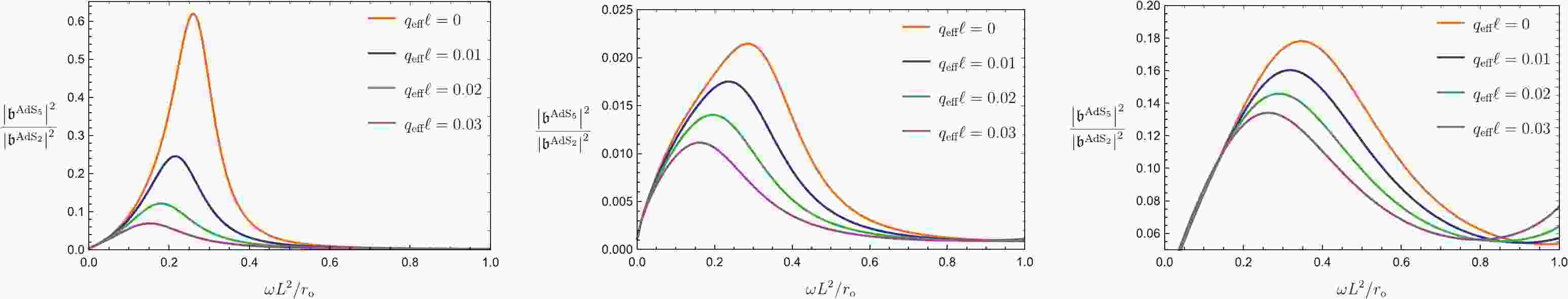
$ |\nu| $ and$ |\Delta| $ .With Eq. (80) at hand we can easily investigate the relationship between the pair production rate in the near horizon and that for the whole spacetime of RN-AdS5. As shown in Fig. 1, we can see that the mean number of produced pairs for the whole spacetime is less than that from near horizon region. Moreover, with increasing charge of the scalar field, the corresponding ratio becomes smaller, which is consistent with previous assumptions stating that the Schwinger effect mainly occurs in the near horizon region.
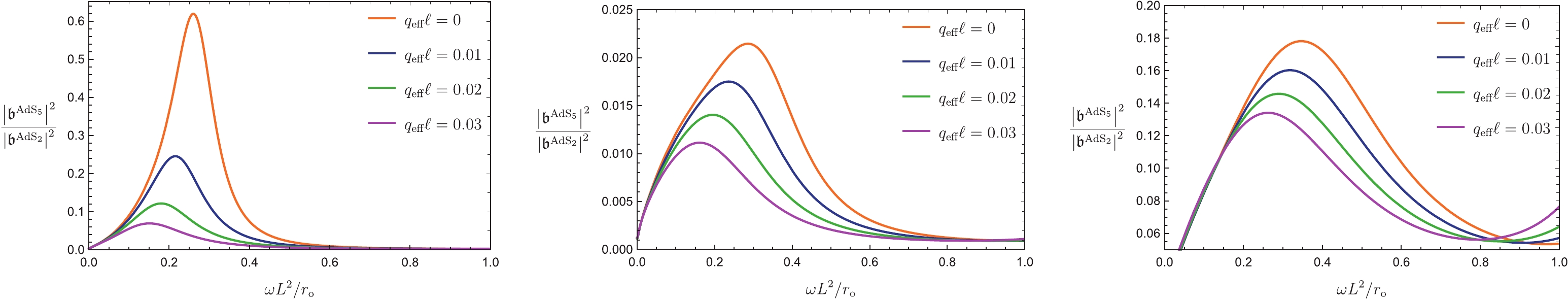
Figure 1. (color online) Ratio of mean number of produced pairs for the whole spacetime to that in the near horizon region as a function of
$ \omega {L^2}/{r_{\rm{o}}} $ for different values of$ {q_{{\rm{eff}}}}\ell $ with$ T{L^{\text{2}}}/{{r_{\text{o}}}} = 0.001 $ ,$ \nu = 0.1{\rm i} $ , and$ \Delta = 0.1{\rm i} $ (left);$ T{L^{\text{2}}}/{{r_{\text{o}}}} = 0.001 $ ,$ \nu = 0.01{\rm i} $ , and$ \Delta = 0.01{\rm i} $ (middle);$ T{L^{\text{2}}}/{{r_{\text{o}}}} = 0.01 $ ,$ \nu = 0.1{\rm i} $ , and$ \Delta = 0.1i $ (right). -
To calculate the retarded Green's function, an ingoing boundary condition is required, namely
$ c_3 = 0 $ . Then, from Eqs. (72) and (73), the connection relations are$ {c_5} = {\left( { - 1} \right)^{ - 1 + \gamma - \beta - \lambda}}{c_4}\frac{{\Gamma \left( {2 - \gamma } \right)\Gamma \left( {\alpha - \beta } \right)}}{{\Gamma \left( {1 - \gamma + \alpha } \right)\Gamma \left( {1 - \beta } \right)}}, $

(84) $ {c_6} = {\left( { - 1} \right)^{ - 1 + \gamma - \alpha - \lambda}}{c_4}\frac{{\Gamma \left( {2 - \gamma } \right)\Gamma \left( {\beta - \alpha } \right)}}{{\Gamma \left( {1 - \gamma + \beta } \right)\Gamma \left( {1 - \alpha } \right)}}. $

(85) Substituting Eqs. (84) and (85) into Eq. (68) and taking
$ y \to \infty $ , namely the boundary of the AdS5 spacetime, one obtains$ \begin{aligned}[b] A(\tilde \omega ,\tilde k) = & \left( - 1 \right)^{{\rm i} q_{\rm{eff}}\ell - 2\lambda - 1 + \Delta }c_4\bigg( \frac{{\Gamma \left( {2 - \gamma } \right)\Gamma \left( {\alpha - \beta } \right)}}{{\Gamma \left( {1 - \gamma + \alpha } \right)\Gamma \left( {1 - \beta } \right)}}\frac{{\Gamma \left( {\gamma '} \right)\Gamma \left( {\alpha ' - \beta '} \right)}}{{\Gamma \left( {\alpha '} \right)\Gamma \left( {\gamma ' - \beta '} \right)}}+ \frac{{\Gamma \left( {2 - \gamma } \right)\Gamma \left( {\beta - \alpha } \right)}}{{\Gamma \left( {1 - \gamma + \beta } \right)\Gamma \left( {1 - \alpha } \right)}}\frac{{\Gamma \left( {2 - \gamma '} \right)\Gamma \left( {\alpha ' - \beta '} \right)}}{{\Gamma \left( {1 - \gamma ' + \alpha '} \right)\Gamma \left( {1 - \beta '} \right)}} \bigg),\\ \\ B(\tilde{\omega}, \tilde{k}) = & \left( - 1 \right)^{{\rm i} q_{\rm{eff}}\ell - 2\lambda - 1 - \Delta }c_4\bigg( \frac{{\Gamma \left( {2 - \gamma } \right)\Gamma \left( {\alpha - \beta } \right)}}{{\Gamma \left( {1 - \gamma + \alpha } \right)\Gamma \left( {1 - \beta } \right)}}\frac{{\Gamma \left( {\gamma '} \right)\Gamma \left( {\beta ' - \alpha '} \right)}}{{\Gamma \left( {\beta '} \right)\Gamma \left( {\gamma ' - \alpha '} \right)}}+ \frac{{\Gamma \left( {2 - \gamma } \right)\Gamma \left( {\beta - \alpha } \right)}}{{\Gamma \left( {1 - \gamma + \beta } \right)\Gamma \left( {1 - \alpha } \right)}}\frac{{\Gamma \left( {2 - \gamma '} \right)\Gamma \left( {\beta ' - \alpha '} \right)}}{{\Gamma \left( {1 - \gamma ' + \beta '} \right)\Gamma \left( {1 - \alpha '} \right)}} \bigg). \end{aligned} $ 
(86) Therefore, the retarded Green's function of the boundary CFT4 is given by
$ G_R^{\mathrm{AdS_5}}\sim\frac{B(\tilde{\omega}, \tilde{k})}{A(\tilde{\omega}, \tilde{k})} = {\left( { - 1} \right)^{ - 2\Delta }}\frac{{\dfrac{{\Gamma \left( {\alpha - \beta } \right)}}{{\Gamma \left( {1 - \gamma + \alpha } \right)\Gamma \left( {1 - \beta } \right)}}\dfrac{{\Gamma \left( {\gamma '} \right)\Gamma \left( {\beta ' - \alpha '} \right)}}{{\Gamma \left( {\beta '} \right)\Gamma \left( {\gamma ' - \alpha '} \right)}} + \dfrac{{\Gamma \left( {\beta - \alpha } \right)}}{{\Gamma \left( {1 - \gamma + \beta } \right)\Gamma \left( {1 - \alpha } \right)}}\dfrac{{\Gamma \left( {2 - \gamma '} \right)\Gamma \left( {\beta ' - \alpha '} \right)}}{{\Gamma \left( {1 - \gamma ' + \beta '} \right)\Gamma \left( {1 - \alpha '} \right)}}}}{{\dfrac{{\Gamma \left( {\alpha - \beta } \right)}}{{\Gamma \left( {1 - \gamma + \alpha } \right)\Gamma \left( {1 - \beta } \right)}}\dfrac{{\Gamma \left( {\gamma '} \right)\Gamma \left( {\alpha ' - \beta '} \right)}}{{\Gamma \left( {\alpha '} \right)\Gamma \left( {\gamma ' - \beta '} \right)}} + \dfrac{{\Gamma \left( {\beta - \alpha } \right)}}{{\Gamma \left( {1 - \gamma + \beta } \right)\Gamma \left( {1 - \alpha } \right)}}\dfrac{{\Gamma \left( {2 - \gamma '} \right)\Gamma \left( {\alpha ' - \beta '} \right)}}{{\Gamma \left( {1 - \gamma ' + \alpha '} \right)\Gamma \left( {1 - \beta '} \right)}}}}, $

(87) which is further simplified into
$ G_R^{\rm{AdS_5}} \sim {\left( { - 1} \right)^{ - 2\Delta }}\frac{{\Gamma \left( { - 2\Delta } \right)}}{{\Gamma \left( {2\Delta } \right)}}\frac{{H\left( {\nu ;\Delta ;\lambda} \right) + H\left( { - \nu ;\Delta ;\lambda} \right)G_R^{\rm{AdS_2}}}}{{H\left( {\nu ; - \Delta ;\lambda} \right) + H\left( { - \nu ; - \Delta ;\lambda} \right)G_R^{\rm{AdS_2}}}}. $

(88) -
From the AdS/CFT correspondence, the IR CFT1 in the near horizon, near extremal limit and the UV CFT4 at the asymptotic boundary of the RN-AdS5 black hole can be connected by the holographic RG flow [26, 27]. The CFT description of the Schwinger pair production in the IR region of charged black holes has been systematically studied in a series of previous works [3, 4, 6, 7]. Herein, we address the dual CFTs descriptions in the UV region and compare them with those in the IR region.
The IR CFT1 of the RN-AdS black hole is very similar to that of the RN black hole in an asymptotically flat spacetime, as CFT1 can be viewed as a chiral part of CFT2, which has the universal structures in its correlation functions. For instance, the absorption cross section of a scalar operator
$ {\cal O} $ in 2D CFT has the universal form$ \begin{aligned}[b] \sigma \sim & \frac{(2 \pi T_{\rm L})^{2h_{\rm L}-1}}{\Gamma(2 h_{\rm L})} \frac{(2 \pi T_{\rm R})^{2 h_{\rm R}-1}}{\Gamma(2 h_{\rm R})} \sinh\left( \frac{\omega_{\rm L} - q_{\rm L} \Omega_{\rm L}}{2 T_{\rm L}} + \frac{\omega_{\rm R} - q_{\rm R} \Omega_{\rm R}}{2 T_{\rm R}} \right) \\ & \times \left| \Gamma\left( h_{\rm L} + {\rm i} \frac{\omega_{\rm L} - q_{\rm L} \Omega_{\rm L}}{2 \pi T_{\rm L}} \right) \right|^2 \left| \Gamma\left( h_{\rm R} + {\rm i} \frac{\omega_{\rm R} - q_{\rm R} \Omega_{\rm R}}{2 \pi T_{\rm R}} \right) \right|^2, \end{aligned} $

(89) where
$ (h_{\rm L}, h_{\rm R}) $ ,$ (\omega_{\rm L}, \omega_{\rm R}) $ , and$ (q_{\rm L}, q_{\rm R}) $ are the left- and right-hand conformal weights, excited energies, charges associated with operator$ {\cal O} $ , respectively, while$ (T_{\rm L}, T_{\rm R}) $ and$ (\Omega_{\rm L}, \Omega_{\rm R}) $ are the temperatures and chemical potentials of the corresponding left- and right-hand sectors of the 2D CFT. Further identifying the variations in the black hole area entropy with those of the CFT microscopic entropy, namely$ \delta S_{\rm BH} = \delta S_{\rm CFT} $ , one derives$ \frac{\delta M}{T_H} - \frac{\Omega_H \delta Q}{T_H} = \frac{\omega_{\rm L} - q_{\rm L} \Omega_{\rm L}}{T_{\rm L}} + \frac{\omega_{\rm R} - q_{\rm R} \Omega_{\rm R}}{T_{\rm R}}, $

(90) where the left hand side of Eq. (90) is calculated with coordinate (14), for which
$ \delta M = \xi_{\mathrm o}w $ ,$ \delta Q = q $ ,$ T_H = \tilde{T}_{ n} $ , and$ \Omega_H = 2\mu\ell^2/r_{\mathrm o} $ , and thus, it is equal to$ w/T_{ n}-2\pi q_{\mathrm{eff}}\ell $ . Moreover, the violation of the BF bound in AdS2 makes the conformal weights of the scalar operator$ {\cal O} $ dual to$ \phi $ a complex, which can be chosen as$ h_{\rm L} = h_{\rm R} = \dfrac 1 2+{\rm i}|\nu| $ , even without further knowledge about the central charge and$ (T_{\rm L}, T_{\rm R}) $ of the IR CFT dual to the near extremal RN-AdS5 black hole. One can also see that the absorption cross section ratio (42) in the AdS2 spacetime has the form of Eq. (89) up to some coefficients, depending on the mass and charge of the scalar field.In contrast, the absorption cross section and retarded Green's functions in a general 4D finite temperature CFT cannot be as easily calculated in momentum space as in the 2D CFT. Thus, it is not straightforward to compare the calculations between the bulk gravity and the boundary CFT sides. Nevertheless, from Eqs. (79) and (80), both the absorption cross section ratio
$ \sigma _{\mathrm{abs}}^{\mathrm{AdS_5}} $ and the Schwinger mean number of produced pairs$ \left|\mathfrak{b}^{\mathrm{AdS_5}}\right|^2 $ calculated from the bulk near extremal RN-AdS5 black hole have a simple proportional relation with their counterparts in the near horizon region. Moreover, the violation of the BF bound (77) in AdS5 spacetime indicates the complex conformal weights$ \bar{\Delta} = 2+2{\rm i}|\Delta| $ of the scalar operator$ \bar{{\cal O}} $ in the UV 4D CFT at the asymptotic spatial boundary of the RN-AdS5 black hole, which also indicates that, to have pair production in the full bulk spacetime, the corresponding operators in the UV CFT should be unstable. Interestingly, Eq. (83) shows that under the interchange between the roles of source and operator both in the IR and UV CFTs at the same time, namely$ h_{\rm L,R} = \dfrac12+ $ $ {\rm i}|\nu| \to \dfrac12-{\rm i}|\nu| $ and$ \bar{\Delta} = 2+2{\rm i}|\Delta|\to 2-2{\rm i}|\Delta| $ , the full absorption cross section ratio$ \sigma _{\mathrm{abs}}^{\mathrm{AdS_5}} $ and the Schwinger pair production rate$ \left|\mathfrak{b}^{\mathrm{AdS_5}}\right|^2 $ are interchanged with each other only up to a minus sign. Note that both the charge and the mass of the scalar particle contribute to the conformal weights$ h_{\rm L,R} $ of the scalar operator in the dual IR CFT; however, only the mass contributes to the conformal weight$ \bar{\Delta} $ of the scalar operator in the dual UV CFT. Actually, it can be seen from the expressions of the conformal weights that the non-zero charge and mass for the scalar field are crucial for the violation of the BF bound in the corresponding AdS spacetimes and hence guarantee the existence of the Schwinger pair production. However, when the charge of the particle is zero, there will be no Schwinger effect, except for an exponentially suppressed Hawking radiation in near extremal black holes. -
In this paper, we describe our study of the spontaneous scalar pair production in a near extremal RN-AdS5 black hole that possesses an AdS2 structure in the IR region and an AdS5 geometry in the UV region.
We firstly calculated the mean number of produced pairs (see Eq. (41)) in the near horizon region, which has an AdS2 structure. The retarded Green's function (see Eq. (46)) has also been obtained for this region. Then, we solved the equation for the whole spacetime of the near extremal RN-AdS5 black hole by using the matching technique. The matching condition we chose is the low temperature limit, i.e., the near extremal limit of the black hole. Therefore, the greybody factor in Eq. (79) and the mean number of produced pairs in Eq. (80) for the whole spacetime are not merely valid for the low frequency limit, and one can easily apply our calculation to the RN-dS black hole, which was recently described in the low frequency limit [35]. Moreover, the retarded Green's function for an RN-AdS black hole has been calculated (see Eq. (88)), which again is valid at finite frequency, and its corresponding value has only been investigated in the low frequency limit [31] before. Interestingly, we found that there exists a very explicit relationship between the mean number of produced pairs (see also Eq. (80)) for the whole spacetime and that in the near horizon region, which enables us to easily compare the pair production rates of these two regions. We showed that, for an near-extremal RN-AdS5 black hole, the dominant contribution to the pair production rate mainly comes from the near horizon region, as expected.
Moreover, the CFT descriptions of the pair production are investigated both from the AdS2/CFT1 correspondence in the IR and the AdS5/CFT4 duality in the UV regions, and consistent results and new connections between the pair production rate and the absorption cross section ratio are found, although the related information computed from the finite temperature 4D CFT is incomplete. This work has successfully generalized the study of pair production in charged black holes to the full spacetime and provided new insights for a complete understanding of the pair production process in curved spacetime.
-
We would like to thank Shu Lin, Rong-Xin Miao, and Yuan Sun for useful discussions.
Pair production in Reissner-Nordström-Anti de Sitter black holes
- Received Date: 2021-02-01
- Available Online: 2021-06-15
Abstract: We studied the pair production of charged scalar particles of a five-dimensional near extremal Reissner-Nordström-Anti de Sitter (RN-AdS5) black hole. The pair production rate and the absorption cross section ratio in full spacetime are obtained and are shown to have a concise relation with their counterparts in the near horizon region. In addition, the holographic descriptions of the pair production, both in the IR CFT in the near horizon region and the UV CFT at the asymptotic spatial boundary of the RN-AdS5 black hole, are analyzed in the AdS2/CFT1 and AdS5/CFT4 correspondences, respectively. This work gives a complete description of scalar pair production in a near extremal RN-AdS5 black hole.


 DownLoad: