


 Abstract
 HTML
HTML Reference
 Related
 PDF
PDF


-
Mass is one of the basic properties of nuclei. The nuclear mass formula is important for nuclear physics and related fields in science and technology. Recently, experimental mass measurements have made it possible to determine the masses of very asymmetric isospin (
$ N/Z $ ) [1-4] as well as very heavy nuclei [5, 6] with high precision.To understand many nuclear structure effects and nuclear synthesis processes in astrophysics, it is necessary to have an accurate knowledge of nuclear mass. In addition, the survival probabilities for the
$ xn $ evaporation channels are very sensitive to the model input. For example, the neutron separation energies and fission barriers have to be known with sufficient accuracy. However, it may not be feasible to experimentally determine the masses of all nuclei of interest in nuclear physics and astrophysics in the near future. Therefore, it is necessary to rely on theoretical models of nuclear masses.The seminal work of theoretical mass formula has been proposed by Weizsäcker, Bethe, and Bacher [7, 8] based on the idea of the liquid drop model. In recent years, many approaches have been developed to predict nuclear mass more accurately [9-24]. There are microscopic self-consistent methods, such as the Hartree-Fock-Bogoliubov approach (HFB) using density functional theory based on Skyrme-type or Gogny-type effective interactions [9, 10] and the relativistic mean-field theory (RMF) [11], as well as macroscopic microscopic methods, such as the finite-range droplet model (FRDM) [17, 18], Koura-Tachibana-Uno-Yamada (KTUY) [19], Lublin Strasbourg drop (LSD) [20], and Weizsäcker-Skyrme (WS) mass formula [21-24]. In addition, the macroscopic microscopic model parameters (MMM2003) [25] obtained by fitting the nuclear properties of heavy nuclei are widely used to describe the properties of heavy and superheavy nuclei [25-27]. The macroscopic microscopic approach is much faster than the microscopic self-consistent approaches, at the cost of being non-self-consistent.
Nuclear mass models contain parameters that must be determined to best reproduce the experimental results. To reasonably determine these parameters, various methods [30-36] are used to estimate their uncertainty when calculating the nuclear binding energy. In recent years, deep machine learning has been used to study the mass of atomic nuclei with great success [31, 35, 36]; this also provides a reliable guarantee for future studies of the related properties of atomic nuclei.
Recently, Sobiczewski and Litvinov quantitatively tested the ability of several models to predict nuclear mass [37]. They found that the best accuracy is obtained by the WS* model [22] in all considered regions, where the root mean square (RMS) deviation is reduced to 0.441 MeV. In the WS* model [22], the macroscopic part is expressed as
$E_{\rm LD}\prod(1+b_{k}\beta_{k}^2)$ . The above parabola approximation of the change in macroscopic energies with$ \beta_{k} (k = 2,3....) $ is acceptable near the ground state. However, such constraints limit the use of this macroscopic microscopic model (WS*) when estimating the potential energy surface in deformation space for describing fission or fusion process.It is reasonable to consider deformation dependent nuclear surface energy and Coulomb energy [38, 39], especially for large deformation, to calculate the ground state energy and potential energy surface. This is also the major motivation of the present work. Furthermore, we consider the consistency of the model parameters between the macroscopic and microscopic parts in WS3.2 [21] and the mirror nuclei constraint [22] in WS*.
-
In the macroscopic microscopic mass formulas, the binding energy of nuclei is divided into two parts [38, 39]. The macroscopic part is the liquid drop energy
$ E_{\text{LD}} $ , and the microscopic part$ E_{\text{shell}} $ is the shell correction energy [40, 41]. Considering the effect of deformation on the binding energy, the total binding energy can be written as$ E(Z,A,\beta_k) = E_{\text{LD}}(Z,A,\beta_k)+E_{\text{shell}}(Z,A,\beta_k), $

(1) where
$ A, Z $ are the nuclear mass number and charge number, respectively, and$ \beta_{k} $ are deformation parameters.The liquid drop energy in Eq. (1) is expressed as
$ \begin{aligned}[b] E_{\rm LD} =& a_V A+a_S A^{\frac{2}{3}}B_S+a_C\frac{Z^2}{A^{\frac{1}{3}}}(1-Z^{-\frac{2}{3}})B_C \\ & +a_{\rm sym}I^{2}A+E_\text{pair}. \end{aligned} $

(2) The first term is the volume energy; the second term is the surface energy, in which
$ B_{S} $ is the ratio of the surface energy of the deformed nucleus to that of a spherical one; and the third term is the Coulomb energy, in which$ B_{C} $ is the ratio of the Coulomb energy of the deformed nucleus to that of a spherical one. Detailed expressions for$ B_S $ and$ B_C $ will be given later.We use uniform neutron and proton distributions with sharp cuts. The shape of the nucleus is represented by the function of the polar coordinate angle
$ \theta $ as follows [42]:$ R(\alpha_i,\theta) = \frac{R_0}{\lambda}\left[1+\sum\limits_{i = 1}^{N}\alpha_{2i} P_{2i}(\cos{\theta})\right]. $

(3) Here, N is a cutoff parameter,
$ P_{2i} (\cos{\theta}) $ (i = 1,2, …) is a Legendre polynomial of order$ 2i $ , and$ \alpha_{2i} $ is a parameter that specifies the shape.$ R_0 $ is the radius of the spherical nucleus considered to be equal to the volume of the deformed nucleus.$ \lambda $ is the volume conservation$ \lambda = \left[1+\frac{3}{4\pi} \left(\frac{4\pi}{5} \alpha_2 ^2+\frac{4\pi}{9} \alpha_4 ^2+\frac{4\pi}{13} \alpha_6 ^2\right)+\cdot\cdot\cdot\right]^{1/3}.$

(4) With these constraints, we can write the deformation parameters of nuclear surface energy and Coulomb energy
$ B_S $ and$ B_C $ as$ B_S = 1+\frac{2}{5}\alpha_{2}^2+\alpha_{4}^2+\frac{20}{13}\alpha_{6}^2+\cdot\cdot\cdot $

(5) $ B_C = 1-\frac{1}{5}\alpha_{2}^2-\frac{5}{27}\alpha_{4}^2-\frac{25}{169}\alpha_{6}^2-\cdot\cdot\cdot $

(6) Then, we can use a transformation relation to replace the deformation descriptor
$ \alpha_i $ in the formula with$ \beta_i $ $ \beta_i = \sqrt{4\pi/(2i+1)}\alpha_i,i = 2,4,6 . $

(7) Finally,
$ B_S $ and$ B_C $ can be written as$ B_S = 1+\frac{1}{2\pi}\beta_{2}^2+\frac{9}{4\pi}\beta_{4}^2+\frac{5}{\pi}\beta_{6}^2, $

(8) $ B_C = 1-\frac{1}{4\pi}\beta_{2}^2-\frac{5}{12\pi}\beta_{4}^2-\frac{25}{52\pi}\beta_{6}^2 . $

(9) We only consider the fourth-order, sixteenth-order, and sixty-fourth-order
$ \{\beta_2,\beta_4,\beta_6\} $ deformations in nuclear deformation space.The fourth term in Eq. (2)
$a_{\rm sym}I^{2}A$ is the symmetry energy. In this equation,$a_{\rm sym}$ is the symmetric energy coefficient$a_{\rm sym} = c_{1}\left(1-\dfrac{k}{A^\frac{1}{3}}B_{S}+\dfrac{2-|I|}{2+|I|A}\right)$ , and I is the isospin asymmetry$ I = (N-Z)/A $ [22].The last term in Eq. (2) is the pairing correction, and
$E_{\rm pair} = a_{\rm pair}A^{-\frac{1}{3}}\delta_{np}$ , where$ \delta_{np} $ is expressed as [43]$\begin{array}{*{20}{l}} {{\delta _{{\rm{np}}}} = \;\left\{ {\begin{array}{*{20}{l}} {2 - |I|,\;{\rm{foreven - }}Z,\;{\rm{even - }}N,}\\ {\;\;\;\;\;|I|,\;{\rm{forodd - }}Z,\;{\rm{odd - }}N,}\\ {1 - |I|,\;{\rm{forodd - }}Z,\;{\rm{even - }}N\;{\rm{and}}\;N > Z,}\\ {1 - |I|,\;{\rm{foreven - }}Z,\;{\rm{odd - N}}\;{\rm{and}}\;N < Z,}\\ {\;\;\;\;\;1,\;{\rm{forodd - Z}},\;{\rm{even - }}N\;{\rm{and}}\;N < Z,}\\ {\;\;\;\;\;1,\;{\rm{foreven - }}Z,\;{\rm{odd - }}N\;{\rm{and}}\;N > Z.} \end{array}} \right.} \end{array}$

The shell correction in Eq. (1) is calculated using Strutinsky's method [40, 41], where an axially deformed Hamiltonian is employed and diagonalized using the computer code WSBETA [44]. In this code, the smooth width is taken as
$ \gamma = 1.2\hbar \omega_0 $ , and the average distance between the total shells is$ \hbar \omega_0 = 41A^{1/3} $ . The plateau condition is important for extracting the reliable shell correction energy in Strutinsky's method [45]. To be able to calculate the global nucleus masses, especially for the superheavy nuclei, we choose the largest possible major shell number of the harmonic oscillator basis. In this work, the major shell number of the harmonic oscillator basis is 20, and the orderof the Gauss-Hermite polynomials p is 6. The single particle Hamiltonian is expressed as
$ H = T + V+ V_{ \rm{so}}, $

(10) where
$V_{\rm so}$ is the spin-orbit potential,$ V_{ \rm{so}} = \lambda\left(\frac{\hbar}{2Mc}\right)^2\times\nabla V\cdot(\vec\sigma\times \vec{p}), $

(11) where
$ \lambda $ is the strength of the spin-orbit potential, for proton$ \lambda = \lambda_0(1+Z/A) $ and for neutron$ \lambda = \lambda_0(1+N/A) $ . The form of the deformed Woods-Saxon potential of the deformation is$ V = \frac{V_{ \rm{depth}}}{1+ {\rm{exp}}\left[\dfrac{r-R(\alpha_i,\theta)}{a}\right]}, $

(12) where
$ R(\alpha_i,\theta) $ represents the distance from the origin of the coordinate system to the nuclear surface point along the radius vector$ \vec r $ . Here, a is the diffusion parameter. The potential depth$ V_{ \rm{depth}} $ can be written as$ V_{ \rm{depth}} = V_0\pm V_s I . $

(13) We use a plus sign for protons and a minus sign for neutrons.
$ V_s $ is the isospin-asymmetry part of the potential depth.$ V_{0} $ is a constant, as an adjustable parameter in mass fitting. The isospin asymmetry of potential depth is equal to the symmetrical energy parameter in the macroscopic part [21], which can be expressed as$ V_s\approx a_{ \rm{sym}}. $

(14) For neutrons and protons, the shell correction is calculated separately. We express
$ E_{\text{shell}} $ as the sum of proton and neutron shell corrections, that is,$ E_{\text{shell}} $ =$ E_{\text{shell}}(Z) $ +$ E_{\text{shell}}(N) $ . Considering the constraints of the mirror nucleus, the actual shell correction is$ f E_{\text{shell}} + |I|E_\text{shell}' $ [22], where$ E_\text{shell}' $ represents the shell energy of the mirror nucleus. -
To fit the adjustable parameters, we selected 2314 atomic masses as the training set to refer to the corresponding subset of AME2016 [46], with the number of protons and neutrons greater than or equal to 8 and the mass measurement error less than 150 keV [46]. The nonlinear least squares method is used for fitting, and the fitting results of Eq. (1) are shown in Table 1. In this work, the fitting procedure primarily consists of the following two steps. First, the ground state deformation of each nucleus is given and the minimum RMS deviation is found in the parameter space. This step uses the Levenberg-Marquardt method. Second, we use the set of parameters determined in the previous step to find the lowest energy value of each nucleus in the deformed space. Thus, the ground state deformation and ground state energy of each nucleus are determined. This step uses the Downhill Simplex method. This process is repeated until the desired accuracy is achieved, after which the iteration process is terminated. After fitting, the resulting RMS deviation is 0.447 MeV. Here, we have only 11 independent parameters. Then, we calculate the percentage error between the calculated value and the experimental value, and the calculation method is as follows [34]:
mac para mic para $ a_V $ 

−15.6192 $ V_0 $ 

−49.4867 $ a_S $ 

18.0592 $ r_0 $ 

1.3265 $ a_C $ 

0.7192 a 0.7588 $ c_1 $ 

29.2372 $ \lambda $ 

24.2105 k 1.3543 f 0.6215 $a_{\rm pair}$ 

−5.3661 Table 1. Model parameters of the mass formula.
$ \frac{|\delta B|}{B} = \frac{|B_{\text{exp.}}-B_{\text{cal.}}|}{B_{\text{exp.}}}\times 100{\text{%}} . $

At present, the percentage error between the calculated binding energy and the experimental value is within 0.8%. The maximum error is 0.77%, and there are 2115 nuclei with a deviation of less than 0.1%.
Compared with the number of parameters and the RMS of FRDM, KTUY, LSD, WS, and other similar global mass formulas, our model has fewer parameters. However, it is consistent with the smallest RMS of WS*, as shown in Table 2.
model number of para $ \sigma $ /MeV

our work 11 0.447 WS* 13 0.441 KTUY 34 0.667 FRDM1995 16+22 0.669 FRDM2012 17+21 0.560 LSD 0.698 Table 2. Number of model parameters and RMS for various macroscopic microscopic models.
In order to test the prediction ability of the our mass formula, we take the remaining 60 atomic masses as the testing set to refer to the other subset of AME2016 [46]. These nuclei are also
$ N\geqslant 8 $ ,$ Z\geqslant 8 $ , and the error of mass measurement is larger than 150 keV and less than 400 keV in Ref. [46]. In Table 3, we have compared and listed the RMS values of different macroscopic-microscopic models. The calculation results proposed in this paper are similar to those for WS* and better than the results of other models.mass table $ \sigma $ /MeV testing set

$ \sigma $ /MeV

$ Q_\alpha $ 

our work 0.793 0.373 WS* 0.738 0.263 KTUY 0.895 0.421 FRDM1995 1.088 0.547 FRDM2012 0.965 0.503 Table 3. Calculated RMS for testing set nuclei and
$ \alpha $ decay energy for superheavy nuclei from AME2016 [46] based on different macroscopic microscopic models.Since
$ ^{294}{\rm{Og}} $ was found, no new nuclides have been synthesized in recent years. However, the synthesis of new nuclides has always been of great concern. The new nuclides were discovered by looking at the daughter nuclei after alpha decay.$ \alpha $ decay half-life is sensitive to decay energy. A more accurate calculation of the half-life of alpha decay requires a precise decay energy. Therefore, we calculated 74 superheavy nuclei$ \alpha $ decay energy$ Q_{\alpha} $ [47] using our mass formula. To compare the results with other mass tables, we calculated the RMS between experimental$ Q_{\alpha} $ . In Table 3, we list the calculated results of each mass table of experimental values. Our results are second only to the WS* with respect to the global quality equation. This shows that our work can be applied to experiments as a reference. -
To test the accuracy of our model, we calculate the single and two nucleon separation energies, as well as the shell gaps. The experimental data for single and two nucleon separation energies are taken from AME2016 [46]. It can be seen from Table 4 that the RMS values of 2113 single neutron separation energies and 2057 proton separation energies have no significant difference in different models. However, for 2033 two neutron separation energies and 1943 two proton separation energies, the RMS calculated in this work and WS* is smaller than that of FRDM2012.
mass table our work FRDM2012 WS* $ \sigma $ (MeV)(

$ S_{p} $ )

0.396 0.391 0.397 $ \sigma $ (MeV)(

$ S_{n} $ )

0.322 0.343 0.316 $ \sigma $ (MeV)(

$ S_{2p} $ )

0.374 0.443 0.373 $ \sigma $ (MeV)(

$ S_{2n} $ )

0.332 0.446 0.316 Table 4. Calculated RMS for single proton separation energies (
$ S_{p} $ ), two proton separation energies ($ S_{2p} $ ), single nucleon separation energies ($ S_{n} $ ), and two nucleon separation energies ($ S_{2n} $ ) using different mass models.As mentioned above, the difference between the work in this paper and WS* is the different consideration of deformation factors. Therefore, we compared the deformation energy calculated by the mass formula proposed in this paper with that calculated by WS*. The deformation energy can be written as the difference between the total energy of a spherical nucleus and a ground state nucleus, i.e., [48]
$ E_{\rm def} = E({\rm spherical})-E(gs) $

In Fig. 1, we show the results of the mass formula proposed in this paper with those from WS* for calculating the deformation energy of the nucleus on the
$ \beta $ -stability line. The deformation energies calculated by both models are almost zero at the magic number. When deviating from the phantom number, the calculation results of both models show the same trend because of the use of the same shell correction calculation method. The difference in the deformation energy calculated by the two methods is reflected in the position far from the phantom number, and the calculation results of the mass model proposed in this paper are slightly larger than those of WS*. The reason for the difference is the different consideration of the deformation factor.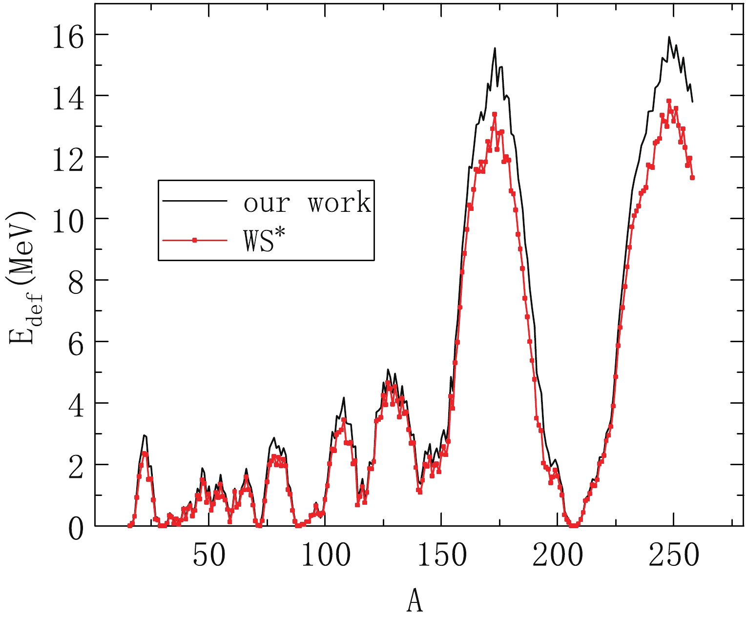
Figure 1. (color online) Deformation energies of nuclei along the
$ \beta $ -stability line. The solid black curve is the calculation result using the work in this paper, and the red solid squares is the calculation result using WS*.The shell gap is a sensitive quantity used to test the theoretical model. The variations of the neutron shell gaps as a function of Z, at the neutron shell closure
$ N_0 $ = 126, 82, 50, and 28, are shown in Figs. 1(a), 1(b), 1(c), and 1(d), respectively. The solid squares in the figures denote experimental data. The solid, dashed, and dotted-dashed lines denote the results of our work, WS*, and FRDM2012, respectively. We can see in Fig. 2 that the experimental shell gaps at magic numbers Z = 20, 28, 40, 50, 82 are remarkably well described with our calculations. Both the present calculation and WS* can describe most of the shell gaps, except for the shell gap at the closure of the sub shell Z = 64. It can be observed from the shell gaps of FRDM1995 that when$ N_{0} $ = 28 and 50, the enhancement of shell structure is approximately reproduced, but it is not at 82 and 126 [49]. Similar results have been obtained from FRDM2012.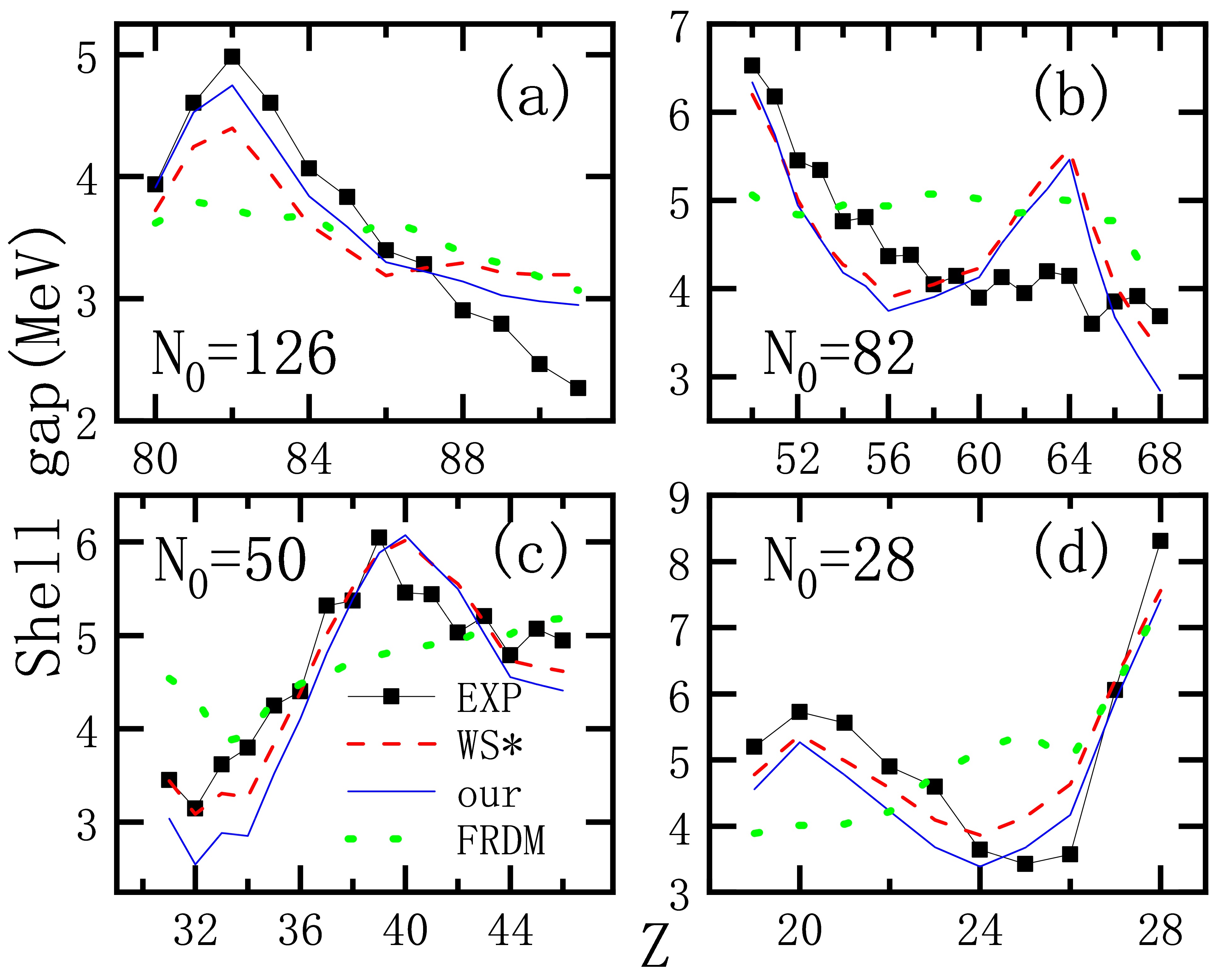
Figure 2. (color online) Shell gaps as a function of Z for the three mass tables from FRDM2012, WS*, and our work for
$ N_{0} $ = 28, 50, 82, and 126. -
Superheavy nuclei production is one of the major aims of low energy heavy-ion collisions. In the study of producing superheavy nuclei by fusion evaporation reaction, the survival probability of the compound nucleus against fission is crucial in the deexcitation process. To precisely estimate the survival probability, basic nuclear data such as the neutron separation energy and the fission barrier must be reliable to some extent.
For superheavy nuclei, neglecting the shell energy at the saddle point [25], the fission barrier can be written as
$ B_{f}\approx B_{\rm LD}-E_{\rm shell}, $

(15) where
$B_{\rm LD}$ and$E_{\rm shell}$ are the macroscopic fission barrier of superheavy nuclei and the shell correction in ground state nuclei, respectively. Because the macroscopic fission barrier generally disappears when$ Z\geq 106 $ , the fission barrier can be roughly estimated using the corresponding nuclear shell correction. Therefore, the fission barriers can be written$ B_{f}\approx -E_{\rm shell},$

(16) In Fig. 3, we show the fission barrier height of even-Z superheavy nuclei calculated with various macroscopic-microscopic models such as FRDM2012 [18], WS* [22], MMM2017 [27], and that in the present work. It can be seen from Fig. 3 that for SHN with
$ Z\geqslant 106 $ , the predicted fission barriers$ B_{f} $ are quite different, and the difference ranges from approximately 1-3 MeV. For some neutron emission channels, a difference in predicted$ B_{f} $ values in the range of 1-3 MeV may lead to a difference in survival probability of one or two orders of magnitude.
Figure 3. (color online) Calculated fission barrier height of even-Z superheavy nuclei from different theoretical models. Our work, MMM2017 [27], FRDM2012, and WS* for fission barriers are denoted by filled black squares, red solid curve, blue hollow circles, and filled pink inverted triangles, respectively.
The fission barrier
$ B_{f} $ strongly depends on the neutron and proton numbers of the compound nucleus, especially on how close they are to the magic numbers. From Fig. 3, we find that the different models give different fission barrier heights, but give the same position as the sub-closed shell$ N_0 = 162 $ when the proton number is relatively small, in the range of$ Z = 106\sim110 $ . With an increase of the number of protons, the shell effect of$ N = 162 $ gradually weakened, and a new magic number appeared. Möller et al. proposed the magic numbers Z = 114 and N = 184 [17], while Wang et al. [22] found that the central position of the stability island of SHN may lie at approximately$ N = 176\sim178 $ and$ Z = 116\sim120 $ . In Fig. 3, it can be seen from the fission barrier height and its variation trend with the neutron number and proton number that when the proton number$ Z = 114\sim118 $ and the neutron number is greater than 170, the fission barrier height is less than that of$ Z = 120 $ with the same neutron number. Because the fission barrier height has a peak at$ Z = 120 $ and$ N = 178 $ , spontaneous fission in the vicinity of this nucleus may be more stable. However, to determine the location of superheavy double magic number nuclei, the single-particle energy levels of the nuclei need to be analyzed. In the next section, we will predict the double magic number nuclei of superheavy nuclei. -
We know that the magic number of nuclei is due to the spin-orbit coupling of the nucleon. The next double magic number nucleus after
$ ^{208}{\rm{Pb}} $ is of interest. By describing the single-particle energy levels of the nucleus, we can determine the position of the double phantom number nucleus in the superheavy nuclear region. First, double magic number nuclei are generally stable spherical nuclei. Therefore, we calculated the nucleus deformation and binding energies in the superheavy nucleus region and found that the three spherical nuclei are$ ^{298} $ Fl,$ ^{304} $ 120, and$ ^{310} $ 126. Next, we calculated the single-particle energy levels of these three nuclei, and after comparing them, we can conclude that$ ^{298} $ Fl is the next double magic number nuclei. The single-particle energy levels of the protons and neutrons of$ ^{298} $ Fl are listed here in Fig. 4. As we can see in Fig. 4, no significant proton shell structure appears, despite the fact that the deformations of$ ^{304} $ 120 and$ ^{310} $ 126 are 0. The most pronounced nucleus shell structure appears for the proton number Z = 114 and neutron number N = 184. That is, our model predicts that the next double magic number nucleus is$ ^{298} $ Fl.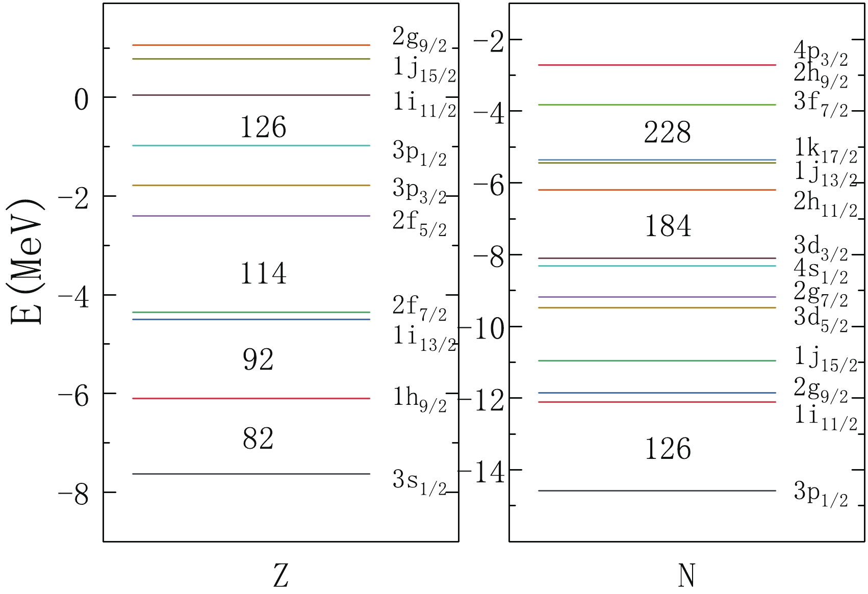
Figure 4. (color online) Single-particle energy levels of
$ ^{298} $ Fl are shown on the left for protons and on the right for neutrons. -
In summary, a mass formula based on the macroscopic microscopic approach has been proposed. The number of model parameters is less than other macroscopic microscopic models; we have only 11 independent parameters. The RMS deviation with respect to 2314 measured nuclear masses is reduced to 0.447 MeV. The RMS of our model is much smaller than those for the FRDM, KTUY, and LSD models. The present result is similar to the accuracy of WS* and employs two parameters less than the number of parameters for WS*. Because of the shape dependence of nuclear surface energy and Coulomb energy, the present model can not only calculate the binding energy of the nucleus but also estimate the potential energy surface in deformation space for describing fission and fusion processes.
The shell gaps at proton magic numbers
$ Z = $ 20, 28, 40, 50, 82 can be remarkably well described with the proposed model. The predicted central position of the superheavy island according to the calculated single-particle energy level of nuclei could lie at approximately$ N = 184 $ and$ Z = 114 $ .As computing power increases, deep machine learning becomes progressively more capable. In our future work, we will combine machine learning with models to pursue more accurate results.
Improved macroscopic microscopic mass formula
- Received Date: 2021-02-07
- Available Online: 2021-07-15
Abstract: A nuclear mass formula based on the macroscopic microscopic approach is proposed, in which the number of model parameters is reduced compared with other macroscopic microscopic models. The root mean square (RMS) deviation with respect to 2314 training sets (measured nuclear masses) is reduced to 0.447 MeV, and the calculated value of each nucleus is no more than 0.8% different from the experimental value. The single and two nucleon separation energies and the shell gaps are calculated to test the model. The shell corrections and double magic number of superheavy nuclei are also analyzed.


 DownLoad: