Processing math: 10%

Effects of an odd particle on shape phase transitions in odd-even systems

  • A scheme to solve the Hamiltonian in the interacting boson-fermion model in terms of the SU(3) coupling basis is introduced, through which the effects of an odd particle on shape phase transitions (SPTs) in odd-A nuclei are examined by comparing the critical behaviors of some selected quantities in odd-even and even-even systems. The results indicate that the spherical to prolate (U(5)-SU(3)) SPT and spherical to γ-soft (U(5)-O(6)) SPT may clearly occur in the odd-even system with the SPT signatures revealed by various quantities including the excitation energies, energy ratio, B(E2) ratio, quadrupole moments, and one-particle-transfer spectroscopic intensities. In particular, the results indicate that the spherical to prolate SPT in the odd-even system can even be strengthened by the effects of the odd particle with the large fluctuations of the quadrupole deformations appearing near the critical point.
  • The Schwinger pair production of charged particles is an important QED phenomenon that is related to the vacuum instability and persistence in the presence of strong external electromagnetic fields [1]. Another important spontaneous pair production phenomenon is the Hawking radiation from black holes, which can be viewed as a tunneling process through the black hole horizon [2]. A charged black hole thus provides a natural lab in which both the Schwinger pair production and the Hawking radiation can occur and mix with each other. Usually the equation of motions (EoMs) of quantum fields in a general black hole background is difficult to solve analytically in full spacetime. However, when the symmetry of the spacetime geometry is enhanced under some conditions, the problem becomes manageable; for this reason, in a series of recent studies, the spontaneous pair production of charged particles has been systematically studied in near extremal charged black holes, including the RN black hole [3-5] and the Kerr-Newman (KN) black hole [6, 7], in which the near horizon geometry is enhanced into AdS2 or warped AdS3 in the near extremal limit. Owing to the enhanced near horizon symmetry, the explicit forms of the pair production rate and other 2-point correlation functions have been obtained and their holographic descriptions have been found based on the RN/CFT [8-13] and KN/CFTs dualities [14-16]. In addition to charged black hole backgrounds, pair production has also been investigated in pure AdS or dS spacetime, see, e.g., [17-20], whereas in the absence of a gravitational field, the pure Schwinger effect has been efficiently analyzed by using the phase-integral method [21-24].

    However, previous studies mainly focused on analyzing spontaneous pair production in the near horizon region of black holes in an asymptotically flat spacetime. A charged black hole in AdS spacetime has an additional AdS symmetry at the asymptotical boundary. From the holographic point of view, the CFT description of pair production has been revealed only in the near horizon region in terms of AdS2/CFT1 (or warped AdS3/CFT2). Although particle pairs produced in the near horizon region of black holes indeed provide important contributions to those in full spacetime, an understanding of the whole picture is still lacking. In the present paper, we extend the study of pair production to a full near extremal RN-AdS5 black hole background, which possesses an AdS5 geometry at the asymptotic spatial boundary as well as an AdS2 structure in the near horizon region. It is shown that the radial equation of the charged scalar field propagating in this spacetime can be transformed into a Heun-like differential equation and thus be solved by matching its solutions in the near and far spacetime regions, using the low temperature limit. Consequently, analytical forms of the full solutions for the pair production rate, the absorption cross section ratio, and the retarded Green's functions are obtained, and they are shown to have concise relations with their counterparts calculated in the near horizon region. Based on these concise relations, numerical analysis can easily be performed, and the pair production rate in full spacetime is shown to be smaller than that in the near horizon region, which is consistent with the assumption that pair production mainly comes from the black hole near horizon region.

    A near extremal RN-AdS5 black hole is also a very useful background for studying holographic dualities. As the near horizon AdS2 (or warped AdS3) spacetime is dual to a 1D CFT (or chiral CFT2), while asymptotical AdS5 spacetime is dual to another 4D CFT, the former is called IR CFT, while the latter is called UV CFT, and they are connected with each other via the holographic renormalization group (RG) flow along the radial direction [25-27]. For example, it has been shown that a near extremal RN-AdS black hole acts as a holographic model in describing typical properties of a (non)Fermi liquid at the quantum critical point [28-31]. It is thus natural and interesting to find holographic descriptions of pair production in an RN-AdS5 black hole both in the IR CFT1 in the near horizon region and the UV CFT4 at the asymptotical AdS5 boundary. We show that the picture in the IR CFT1 is very similar to those in the near extremal RN and KN black holes, and that the pair production rate and the absorption cross section ratio calculated from the AdS2 spacetime can be matched with those from the dual IR CFT. Regarding the UV 4D CFT, a direct comparison of calculations between the bulk and the boundary in terms of the AdS5/CFT4 is not made due to a lack of information on the dual finite temperature CFT4 side. However, from the bulk gravity side, the condition for pair production in the full near extremal RN-AdS5 spacetime is the violation of the Breitenlohner-Freedman (BF) bound [32, 33] in AdS5 spacetime. This, on the dual 4D CFT side, corresponds to a complex conformal weight for the scalar operator dual to the bulk charged scalar field, which indeed indicates instabilities for the scalar operator on the boundary and is consistent with the situation in the IR CFT. Furthermore, we determined an interesting relation between the full pair production rate and the absorption cross section ratio via changing the roles of sources and operators simultaneously both in the IR and the UV CFTs.

    The rest of the paper is organized as follows. In Sec. II, we provide a brief review of the bulk theory and consider the near horizon geometry of an RN- AdSd+1 black hole and the EoMs of the probe charged scalar field. In Sec. III, spontaneous pair production in the near horizon region of near extremal RN- AdSd+1 black holes is discussed, and the 2-point functions of the charged scalar field (such as the retarded Green's function), pair production rate, and absorption cross section ratio are calculated. In Sec. IV, the full analytical solution for the radial equation of the charged scalar field in RN-AdS5 black holes is obtained by applying the matching technique. Consequently, the full analytical forms of the pair production rate, absorption cross section ratio, and retarded Green's function are found, and the connections with their counterparts in the near horizon region of the black hole are discussed. Then, in Sec. V, the dual CFTs descriptions of spontaneous pair production are both analyzed in terms of the AdS2/CFT1 correspondence in the IR region and the AdS5/CFT4 correspondence in the UV region, and their connections are also revealed. Finally, the conclusion and physical implications are provided in Sec. VI.

    The d+1 dimensional Einstein-Maxwell theory has an action (in units of c==1) as

    I=dd+1xg[116πGd+1(R+d(d1)L2)1g2sFμνFμν],

    (1)

    where L is the curvature radius of the asymptotical AdSd+1 spacetime, and gs is the dimensionless coupling constant of the U(1) gauge field. The dynamical equations

    Rμν12gμνRd(d1)2L2gμν=8πGd+1g2s(4FμλFνλgμνFαβFαβ),μ(gFμν)=0,

    (2)

    admit the Reissner-Nordström-Anti de Sitter (RN-AdSd+1) black brane (or the planar black hole) solution [34]

    ds2=L2r2f(r)dr2+r2L2(f(r)dt2+dx2i),A=μ(1rd2ord2)dt,

    (3)

    with

    f(r)=1Gd+1L2Mrd+Gd+1L2Q2r2d2,μ=d12(d2)gsQrd2o,

    (4)

    where ro is the radius of the outer horizon (f(ro)=0), μ is the chemical potential with dimension [μ]=length(d1)/2, M is the mass, and Q is the charge of the black brane. We may find an explicit expression of ro for d=4 from a solution of the cubic equation, which is complicated, but ro has a general expression in the extremal case, i.e., r in IIB. The condition f(ro)=0 gives M=rdoGd+1L2+Q2rd2o (which is the Smarr-like relation related to the first law of thermodynamics of the black brane); temperature T and “surface” entropy density s of the black brane are, respectively,

    T=rod4πL2(1d2dGd+1L2Q2r2d2o),s=14Gd+1(roL)d1.

    (5)

    Moreover, the first law of thermodynamics of the dual boundary d-dimensional quantum field is

    δϵ=Tδs+μδρc,

    (6)

    where the “surface” energy and charge densities are, respectively,

    ϵ=d116πLd1M,ρc=2(d1)(d2)8πgsLd1Q.

    (7)

    Then, it is straightforward to check the Euler relation

    (dd1)ϵ=ϵ+p=Ts+μρc,

    (8)

    where the pressure is p=ϵd1, which shows that the dual d-dimensional quantum field theory on the asymptotic boundary is conformal, as expected.

    To make the following analysis convenient, let us introduce the length scale r2d2d2dGd+1L2Q2; then, the temperature can be rewritten as

    T=rod4πL2(1r2d2r2d2o).

    (9)

    Note that r may be treated as the “effective” radius of the inner black hole horizon though f(r)0 in general and r<ro. The extremal condition for a degenerate horizon at ro=r is M=M02(d1)d2rdGd+1L2. The near extremal limit of the near horizon is obtained by taking the limit ε0 of the transformations

    MM0=d(d1)rd2Gd+1L2ε2ρ2o,ror=ερo,rro=ε(ρρ0),t=τε,

    (10)

    where in general ρo is finite and ρ[ρ0,).

    Expanding f(r) around r=ro, we have

    f(r)d(d1)r2o(ρ2ρ2o)ε2+O(ε3),

    (11)

    the near horizon geometry is given by

    ds2=ρ2ρ2o2dτ2+2dρ2ρ2ρ2o+r2oL2dx2i,A=(d2)μro(ρρo)dτ,

    (12)

    where 2L2d(d1) is defined as the square of the curvature radius of the effective AdS2 geometry. The limit ρo0 yields the extremal limit.

    The solution in Eq. (12) can also be written in the Poincaré coordinates in terms of ξ=2/ρ, (|ξ| \ell^2/\rho_\mathrm{o} ),

    \begin{aligned}[b] {\rm d}s^2 & = \frac{\ell^2}{\xi^2} \left( - \left( 1 - \frac{\xi^2}{\xi_{\mathrm o}^2} \right) {\rm d}\tau^2 + \frac{{\rm d}\xi^2}{1-\dfrac{\xi^2}{\xi_{\mathrm o}^2}} \right) + \frac{r_{\mathrm o}^2}{L^2} {\rm d}x_i^2, \\ A & = \frac{(d-2) \mu \ell^2}{r_{\mathrm o}} \left( \frac{1}{\xi} - \frac{1}{\xi_{\mathrm o}} \right) {\rm d}\tau. \end{aligned}

    (13)

    The above geometry is a black brane with both local and asymptotical topology {\rm{AdS}}_2 \times {{R}}^{d-1} (AdS2 has the SL(2,R)_R symmetry). The horizons of the new black brane are located at \xi = \pm \xi_{\mathrm o} , and its temperature is T_{ {{n}}} = \dfrac{1}{2 \pi \xi_{\mathrm o}} . Note that if we adopt the new coordinates z \equiv \xi/\xi_{\mathrm o} with |z| \leqslant 1 and \eta = \tau/\xi_{\mathrm o} , the metric becomes

    {\rm d}s^2 = \frac{\ell^2}{z^2} \left( - (1 - z^2) {\rm d}\eta^2 + \frac{{\rm d}z^2}{1-z^2} \right) + \frac{r_{\mathrm o}^2}{L^2} {\rm d}x_i^2,

    (14)

    and the temperature associated with the inverse period of \eta is normalized to \tilde{T}_{ n} = \dfrac{1}{2\pi} .

    The action of a bulk probe charged scalar field \Phi with mass m and charge q is

    S = \int {{{\rm d}^{d + 1}}} x\sqrt { - g} \left( { - \frac{1}{2}{D_\alpha^* }{\Phi ^*}{D^\alpha }\Phi - \frac{1}{2}{m^2}{\Phi ^*}\Phi } \right),

    (15)

    where D_{\alpha} \equiv \nabla_{\alpha} - {\rm i} q A_{\alpha} with \nabla_\alpha being the covariant derivative in curved spacetime. The corresponding Klein-Gordon (KG) equation is

    (\nabla_\alpha - {\rm i} q A_\alpha) (\nabla^\alpha - {\rm i} q A^\alpha) \Phi = m^2 \Phi.

    (16)

    Moreover, the radial flux of the probe field is

    {\cal F} = {\rm i}\sqrt { - g} {g^{rr}}(\Phi D_r^*{\Phi ^*} - {\Phi ^*}{D_r}\Phi ).

    (17)

    In the RN- {\rm{AdS}}_{d+1} background (3), assuming \Phi(t, \vec{x}, r) = \phi(r) \mathrm{e}^{-{\rm i} \omega t + {\rm i} \vec{k} \cdot \vec{x}} , the KG Eq. (16) has the radial form

    \begin{aligned}[b]& \left(\frac{L}{r}\right)^{d-1} \partial_r \left( \frac{r^{d+1}}{L^{d+1}} f(r) \partial_r \right) \phi(r) \\& + \left(\frac{L^2 (\omega + q A_t)^2}{r^2 f(r)} - m^2 - \frac{L^2}{r^2} \vec{k}^2 \right) \phi(r) = 0. \end{aligned}

    (18)

    The solutions to Eq. (18) cannot be directly found in terms of special functions in the full spacetime region. In what follows, we solve it in different regions and match these solutions to obtain the full solution.

    Firstly, we analyze the near horizon, near extreme region (13) and solve the KG Eq. (16) by expanding the scalar field as

    \Phi(\tau, \vec{x}, \xi) = \phi(\xi) \mathrm{e}^{-{\rm i} w \tau + {\rm i} \vec{k} \cdot \vec{x}}.

    (19)

    Then, the KG equation reduces to

    \begin{aligned}[b] \xi^2 \left( 1 - \frac{\xi^2}{\xi_{\mathrm o}^2} \right) \phi''(\xi) - \frac{2\xi^3}{\xi_{\mathrm o}^2} \phi'(\xi) + \xi^2 \frac{(w + q A_\tau)^2}{1 - \dfrac{\xi^2}{\xi_{\mathrm o}^2}} \phi(\xi) = m_\mathrm{eff}^2 \ell^2 \phi(\xi), \end{aligned}

    (20)

    where the effective mass square is defined as m_\mathrm{eff}^2 = m^2 + \dfrac{L^2 \vec{k}^2}{r_{\mathrm o}^2} , or the KG equation can be expressed in the z coordinate as

    \begin{aligned}[b] z^2 (1 - z^2) \phi''(z) - 2 z^3 \phi'(z) &+ \frac{z^2}{1 - z^2} \left[ \left( w \xi_{\mathrm o} + q_\mathrm{eff} \ell \frac{1 - z}{z} \right)^2\right. \\&\left.- m_\mathrm{eff}^2 \ell^2 \frac{1 - z^2}{z^2} \right] \phi(z) = 0, \end{aligned}

    (21)

    where the effective charge of the probe field is q_\mathrm{eff} \equiv (d-2) \dfrac{\mu \ell}{r_{\mathrm o}} q . The singularities of Eq. (21) are located at z = 0, z = \pm 1 and z = \infty .

    To find the solutions, we determine the indices at each singular point. For z \to 0 , setting \phi(z) \sim z^{\bar{\alpha}} , the leading terms in Eq. (21) are

    z^2 \phi''(z) + (q_\mathrm{eff}^2 - m_\mathrm{eff}^2) \ell^2 \phi(z) = 0,

    (22)

    which gives

    \begin{aligned}[b] \bar{\alpha} = &\frac12 \pm \frac12 \sqrt{1 + 4 ( m_\mathrm{eff}^2 - q_\mathrm{eff}^2 ) \ell^2} \\\equiv &\frac12 \pm \frac12 \sqrt{1 + 4 \tilde{m}_\mathrm{eff}^2 \ell^2} \equiv \frac12 \pm \nu. \end{aligned}

    (23)

    For z \to -1 , setting \phi(z) \sim (1 + z)^{\bar{\beta}} , Eq. (21) reduces to

    2 (1 + z) \phi''(z) + 2 \phi'(z) + \frac{(w \xi_{\mathrm o} - 2 q_\mathrm{eff} \ell)^2}{2 (1 + z)} \phi(z) = 0,

    (24)

    and the index is

    \bar{\beta} = \pm {\rm i} \left( \frac{w \xi_{\mathrm o}}{2} - q_\mathrm{eff} \ell \right) = \pm {\rm i} \left( \frac{w}{4 \pi T_{\mathrm n}} - q_\mathrm{eff} \ell \right).

    (25)

    Finally, for z \to 1 , setting \phi(z) \sim (1 - z)^{\bar{\gamma}} , Eq. (21) reduces to

    2 (1 - z) \phi''(z) - 2 \phi'(z) + \frac{(w \xi_{\mathrm o})^2}{2 (1 - z)} \phi(z) = 0,

    (26)

    from which

    \bar{\gamma} = \pm {\rm i} \frac{w \xi_{\mathrm o}}{2} = \pm {\rm i} \frac{w}{4 \pi T_{\mathrm n}} = \pm {\rm i}\frac{\omega/\varepsilon}{4\pi /(2\pi \xi_{\mathrm o})} = \pm {\rm i}\frac{\omega}{2\varepsilon\rho_{\mathrm o}/\ell^2} = \pm {\rm i}\frac{\omega}{4\pi T}

    (27)

    is obtained. Further, imposing the ingoing boundary condition at the black brane horizon z = 1 requires \bar{\gamma} = -{\rm i} \dfrac{w \xi_{\mathrm o}}{2} = -{\rm i} \dfrac{w}{4\pi T_{\mathrm n}} .

    Also, note that Eq. (21) can be rewritten in a more explicit form as

    \begin{aligned}[b] \phi''(z) + \left( \frac{1}{z+1} + \frac{1}{z-1} \right) \phi'(z) + \left( \frac{\tilde{m}_\mathrm{eff}^2 \ell^2}{z} + \frac{\dfrac{1}{2} (w \xi_{\mathrm o} - 2 q_\mathrm{eff} \ell)^2}{z+1} + \frac{\dfrac12 w^2 \xi_{\mathrm o}^2}{z-1} \right) \frac{\phi(z)}{z (z+1) (z-1)} = 0, \end{aligned}

    (28)

    which becomes the Fuchs equation with three canonical singularities a_1 , a_2 and a_3 , as follows:

    \begin{aligned}[b] \phi''(z) &+ \left( \frac{1-\bar{\alpha}_1-\bar{\alpha}_2}{z-a_1} + \frac{1-\bar{\beta}_1-\bar{\beta}_2}{z-a_2} + \frac{1-\bar{\gamma}_1-\bar{\gamma}_2}{z-a_3} \right) \phi'(z) + \left( \frac{\bar{\alpha}_1 \bar{\alpha}_2 (a_1-a_2) (a_1-a_3)}{z-a_1} + \frac{\bar{\beta}_1 \bar{\beta}_2 (a_2-a_3) (a_2-a_1)}{z-a_2}\right. \\&\left.+ \frac{\bar{\gamma}_1 \bar{\gamma}_2 (a_3-a_1) (a_3-a_2)}{z-a_3} \right) \frac{\phi(z)}{(z-a_1)(z-a_2)(z-a_3)} = 0, \end{aligned}

    (29)

    where a_1 = 0 , a_2 = -1 , and a_3 = 1 and

    \begin{aligned}[b]& \bar{\alpha}_1 = \frac12 \pm \nu, \quad \bar{\alpha}_2 = \frac12 \mp \nu, \quad \bar{\beta}_1 = - \bar{\beta}_2 = \pm {\rm i} \frac{w \xi_{\mathrm o} - 2 q_\mathrm{eff} \ell}2, \\& \bar{\gamma}_1 = - \bar{\gamma}_2 = \pm {\rm i} \frac{w \xi_{\mathrm o}}2, \end{aligned}

    (30)

    and \bar{\alpha}_1 + \bar{\alpha}_2 + \bar{\beta}_1 + \bar{\beta}_2 + \bar{\gamma}_1 + \bar{\gamma}_2 = 1 is satisfied. The Fuchs Eq. (29) can be transformed into the standard hypergeometric function

    \zeta (1 - \zeta) \psi''(\zeta) + \left[ \tilde{\gamma} - (1 + \tilde{\alpha} + \tilde{\beta}) \zeta \right] \psi'(\zeta) - \tilde{\alpha} \tilde{\beta} \psi(\zeta) = 0,

    (31)

    via the conformal coordinate transformation

    \zeta = \frac{(a_2-a_3)(z-a_1)}{(a_2-a_1)(z-a_3)}, \quad {\rm{}} \;\; \phi(z) = \left(\frac{z-a_1}{z-a_3}\right)^{\bar{\alpha}_1} \left(\frac{z-a_2}{z-a_3}\right)^{\bar{\beta}_1} \psi(\zeta),

    (32)

    where \tilde{\alpha} = \bar{\alpha}_1 + \bar{\beta}_1 + \bar{\gamma}_1, \tilde{\beta} = \bar{\alpha}_1 + \bar{\beta}_1 + \bar{\gamma}_2 and \tilde{\gamma} = 1 + \bar{\alpha}_1 - \bar{\alpha}_2 . (Note that one can freely choose the indices i = 1,\; 2 for \bar{\alpha}_i , \bar{\beta}_i and \bar{\gamma}_i .)

    For Eq. (28), we have \zeta = 2z/(z-1) ,\tilde{\alpha} = \dfrac12 \pm \nu + {\rm i} w \xi_{\mathrm o} - {\rm i} q_\mathrm{eff} \ell, \;\;\;\;\tilde{\beta} = \dfrac12 \pm \nu - {\rm i} q_\mathrm{\rm eff} \ell, \;\;\;\; \tilde{\gamma} = 1 \pm 2\nu. Therefore, the explicit solutions in the near horizon near extreme region are

    \begin{aligned}[b] \phi(z) =& c_1 \left(\frac{z}{z-1}\right)^{\frac12 + \nu} \left(\frac{z+1}{z-1}\right)^{{\rm i} \frac{w \xi_{\mathrm o}}{2} - {\rm i} q_\mathrm{eff} \ell} {_2F_1}\left(\frac12 + \nu + {\rm i} w \xi_{\mathrm o} - {\rm i} q_\mathrm{eff} \ell, \frac12 + \nu - {\rm i} q_\mathrm{eff} \ell; 1 + 2 \nu; \frac{2z}{z-1} \right) \\ & + c_2 \left(\frac{z}{z-1}\right)^{\frac12 - \nu} \left(\frac{z+1}{z-1}\right)^{{\rm i} \frac{w \xi_{\mathrm o}}{2} - {\rm i} q_\mathrm{eff} \ell} {_2F_1}\left(\frac12 - \nu + {\rm i} w \xi_{\mathrm o} - {\rm i} q_\mathrm{eff} \ell, \frac12 - \nu - {\rm i} q_\mathrm{eff} \ell; 1 - 2 \nu; \frac{2z}{z-1} \right).\\ \end{aligned}

    (33)

    At the horizon of the AdS2 black brane, z = 1 , Eq. (33) is expanded as follows:

    \phi(z) = c_H^{(\mathrm {in})}(1-z)^{-{\rm i} \frac{w}{4\pi T_{ n}}} + c_H^{(\mathrm {out})} (1-z)^{{\rm i} \frac{w}{4\pi T_{n}}},

    (34)

    where

    \begin{aligned}[b] c_H^{(\mathrm {in})} = c_1 (-)^{-\frac12 - \nu - {\rm i} \frac{w}{2 \pi T_{ n}} + {\rm i} q_\mathrm{eff} \ell} \, 2^{-\frac12 - \nu + {\rm i} \frac{w}{4\pi T_{ n}}} \frac{\Gamma\left(1 + 2\nu\right) \Gamma\left({\rm i} \dfrac{w}{2\pi T_{ n}}\right)}{\Gamma\left(\dfrac12 + \nu + {\rm i} q_\mathrm{eff} \ell\right) \Gamma\left(\dfrac12 + \nu + {\rm i} \dfrac{w}{2\pi T_{ n}} - {\rm i} q_\mathrm{eff} \ell\right)}\end{aligned}

    \begin{aligned}[b]+ c_2 (-)^{-\frac12 + \nu - {\rm i} \frac{w}{2 \pi T_{ n}} + {\rm i} q_\mathrm{eff} \ell} \, 2^{-\frac12 + \nu + {\rm i} \frac{w}{4\pi T_{ n}}} \frac{\Gamma\left(1 - 2\nu\right) \Gamma\left({\rm i} \dfrac{w}{2\pi T_{ n}}\right)}{\Gamma\left(\dfrac12 - \nu + {\rm i} q_\mathrm{eff} \ell\right) \Gamma\left(\dfrac12 - \nu + {\rm i} \dfrac{w}{2\pi T_{ n}} - {\rm i} q_\mathrm{eff} \ell\right)}, \end{aligned}

    (35)

    and

    \begin{aligned}[b] c_H^{(\mathrm {out})} =& c_1 (-)^{-\frac12 - \nu - {\rm i} \frac{w}{2 \pi T_{ n}} + {\rm i} q_\mathrm{eff} \ell} \, 2^{-\frac12 - \nu - {\rm i} \frac{w}{4 \pi T_{ n}}} \frac{\Gamma\left(1 + 2\nu\right) \Gamma\left(-{\rm i} \dfrac{w}{2\pi T_{ n}}\right)}{\Gamma\left(\dfrac12 + \nu - {\rm i} q_\mathrm{eff} \ell\right) \Gamma\left(\dfrac12 + \nu - {\rm i} \dfrac{w}{2\pi T_{n}} + {\rm i} q_\mathrm{eff} \ell\right)} \\ &+ c_2 (-)^{-\frac12 + \nu - {\rm i} \frac{w}{2 \pi T_{ n}} + {\rm i} q_\mathrm{eff} \ell} \, 2^{-\frac12 + \nu - {\rm i} \frac{w}{4\pi T_{ n}}} \frac{\Gamma\left(1 - 2\nu\right) \Gamma\left(-{\rm i} \dfrac{w}{2\pi T_{ n}}\right)}{\Gamma\left(\dfrac12 - \nu - {\rm i} q_\mathrm{eff} \ell\right) \Gamma\left(\dfrac12 - \nu - {\rm i} \dfrac{w}{2\pi T_{ n}} + {\rm i} q_\mathrm{eff} \ell\right)}. \end{aligned}

    (36)

    In contrast, at the AdS2 boundary, z \rightarrow 0 , the asymptotic expansion of Eq. (33) is

    \begin{aligned}[b] \phi(z) =& c_2 (-)^{\frac12 - \nu + {\rm i} \frac{w}{4\pi T_{ n}} - {\rm i} q_\mathrm{eff} \ell} z^{\frac{1}{2}- \nu} + c_1 (-)^{\frac12 + \nu + i \frac{w}{4\pi T_{\mathrm n}} - {\rm i} q_\mathrm{eff} \ell} z^{\frac{1}{2}+ \nu} \\=& {\cal A}(w, \vec{k})z^{\frac{1}{2}- \nu}+{\cal B}(w, \vec{k})z^{\frac{1}{2}+ \nu},\end{aligned}

    (37)

    where {\cal A} is the source of the charged scalar field in the bulk AdS2, while {\cal B} is the response or the operator {\cal \hat{O}}(w,\vec{k}) (in the momentum space) of the boundary CFT1 (i.e., the IR CFT) dual to the charged scalar field in the bulk AdS2 background. Note that in order to obtain the propagating modes, \nu should be purely imaginary, which can be set as \nu \equiv {\rm i} |\nu| , i.e., \phi(z) = c_B^{(\mathrm {out})} z^{\frac{1}{2} - {\rm i}|\nu|} + c_B^{(\mathrm {in})} z^{\frac{1}{2} + {\rm i}|\nu|} . It was shown in [3] that the condition of an imaginary \nu is equivalent to the violation of the BF bound in AdS2 spacetime, namely

    \begin{aligned} \tilde{m}_\mathrm{eff}^2 < -\frac{1}{4\ell^2}, \end{aligned}

    (38)

    which corresponds to a complex conformal weight of the scalar operator in the dual IR CFT.

    1   Pair production rate and absorption cross section ratio

    The Schwinger pair production rate |\mathfrak{b}|^2 and the absorption cross section ratio \sigma_{\mathrm{abs}} can be calculated from the radial flux by imposing different boundary conditions

    \begin{align} {\cal F} = {\rm i} \left(\frac{r_{\mathrm o}}{L}\right)^{d-1} (1-z^2) (\Phi \partial_z \Phi^* - \Phi^* \partial_z \Phi), \end{align}

    (39)

    which gives

    \begin{aligned}[b] {\cal F}_B^{(\mathrm {in})} =& 2 |\nu| \left(\frac{r_{\mathrm o}}{L}\right)^{d-1} |c_B^{(\mathrm {in})}|^2,\\ {\cal F}_B^{(\mathrm {out})} =& -2 |\nu| \left(\frac{r_{\mathrm o}}{L}\right)^{d-1} |c_B^{(\mathrm {out})}|^2, \\ {\cal F}_H^{(\mathrm {in})} =& \frac{w}{2\pi T_{\mathrm n}} \left(\frac{r_{\mathrm o}}{L}\right)^{d-1} |c_H^{(\mathrm {in})}|^2, \\ {\cal F}_H^{(\mathrm {out})} =& -\frac{w}{2\pi T_{\mathrm n}} \left(\frac{r_{\mathrm o}}{L}\right)^{d-1} |c_H^{(\mathrm {out})}|^2, \end{aligned}

    (40)

    where {\cal F}_B^{(\mathrm {in})} and {\cal F}_B^{(\mathrm {out})} are the ingoing and outgoing fluxes at the AdS2 boundary, while {\cal F}_H^{(\mathrm {in})} and {\cal F}_H^{(\mathrm {out})} are the ingoing and outgoing fluxes at the AdS2 black brane horizon, respectively.

    The Schwinger pair production rate {{{\left| {{\mathfrak{b}^{{\text{Ad}}{{\text{S}}_{\text{2}}}}}} \right|}^{\text{2}}}} can be computed either by choosing the inner boundary condition or the outer boundary condition, which gives the same result [3], e.g., by adopting the outer boundary condition, i.e., {\cal F}_B^{(\mathrm {in})} = 0 , ( c_B^{(\mathrm {in})} = 0 \Rightarrow c_1 = 0 ),

    \begin{aligned}[b] {{{\left| {{\mathfrak{b}^{{\text{Ad}}{{\text{S}}_{\text{2}}}}}} \right|}^{\text{2}}}}& = \frac{{\cal F}_B^{(\mathrm {out})}}{{\cal F}_H^{(\mathrm {in})}} = \frac{4 \pi T_{ n} |\nu|}{w} \left|\frac{c_B^{(\mathrm {out})}}{c_H^{(\mathrm {in})}}\right|^2 = \frac{ 8 \pi T_{ n} |\nu|}{w} \left| \frac{\Gamma\left(\dfrac12 - {\rm i}|\nu| + {\rm i} q_\mathrm{eff} \ell\right) \Gamma\left(\dfrac12 - {\rm i}|\nu| + {\rm i} \dfrac{w}{2\pi T_{ n}} -{\rm i} q_\mathrm{eff} \ell\right)}{\Gamma\left(1 - 2{\rm i}|\nu|\right) \Gamma\left({\rm i} \dfrac{w}{2\pi T_{ n}}\right)}\right|^2\\ & = \frac{2\sinh\left(2\pi|\nu| \right)\sinh\left(\dfrac{w}{2T_{ n}}\right)}{\cosh\pi\left(|\nu|-q_\mathrm{eff} \ell\right)\cosh\pi\left(|\nu|-\dfrac{w}{2\pi T_{ n}}+q_\mathrm{eff} \ell\right)}. \end{aligned}

    (41)

    Similarly, by adopting the outer boundary condition, the absorption cross section ratio is computed as

    \begin{aligned}[b] \sigma _{{\text{abs}}}^{{\text{Ad}}{{\text{S}}_{\text{2}}}}& = \frac{{\cal F}_B^{(\mathrm {out})}}{{\cal F}_H^{(\mathrm {out})}} = \frac{4 \pi T_{ n} |\nu|}{w} \left|\frac{c_B^{(\mathrm {out})}}{c_H^{(\mathrm {out})}}\right|^2 = \frac{ 8 \pi T_{ n} |\nu|}{w} \left| \frac{\Gamma\left(\dfrac12 - {\rm i}|\nu| - {\rm i} q_\mathrm{eff} \ell\right) \Gamma\left(\dfrac12 - {\rm i}|\nu| - {\rm i} \dfrac{w}{2\pi T_{ n}} +{\rm i} q_\mathrm{eff} \ell\right)}{\Gamma\left(1 - 2{\rm i}|\nu|\right) \Gamma\left(-{\rm i} \dfrac{w}{2\pi T_{ n}}\right)}\right|^2\\ & = \frac{2\sinh\left(2\pi|\nu| \right)\sinh\left(\dfrac{w}{2T_{ n}}\right)}{\cosh\pi\left(|\nu|+q_\mathrm{eff} \ell\right)\cosh\pi\left(|\nu|+\dfrac{w}{2\pi T_{ n}}-q_\mathrm{eff} \ell\right)}. \end{aligned}

    (42)

    The pair production rate and the absorption cross section ratio are connected by the simple relation

    {{{\left| {{\mathfrak{b}^{{\text{Ad}}{{\text{S}}_{\text{2}}}}}} \right|}^{\text{2}}}} =-\sigma_{\mathrm{abs}}(|\nu|\rightarrow -|\nu|).

    (43)

    It was shown that the abovementioned relation also holds for a charged scalar field [11] and for a charged spinor field [4], both in a four-dimensional near extremal RN black hole.

    2   Retarded Green's function

    The two-point retarded Green's function of the boundary operator dual to the bulk charged scalar field is computed through

    \begin{aligned}[b] G_R^{\mathrm {AdS_2}}(w, \vec{k}) \equiv & \langle {\cal \hat{O}} {\cal \hat{O}} \rangle_R\\ =& -2 {\cal F}|_{z\rightarrow 0} \sim \frac{{\cal B}(w, \vec{k})}{{\cal A}(w, \vec{k})} \\&+ \rm{contact\; terms} \end{aligned}

    (44)

    by taking the inner boundary condition, i.e., {\cal F}_H^{(\mathrm {out})} = 0 , which gives

    \frac{c_2}{c_1} = (-)^{1 - 2\nu} \, 2^{-2\nu} \frac{\Gamma\left(1 + 2\nu\right) \Gamma\left(\dfrac12 - \nu - {\rm i} q_\mathrm{eff} \ell\right) \Gamma\left(\dfrac12 - \nu - {\rm i} \dfrac{w}{2\pi T_{\mathrm n}} + {\rm i} q_\mathrm{eff} \ell\right)}{\Gamma\left(1 - 2\nu\right) \Gamma\left(\dfrac12 + \nu - {\rm i} q_\mathrm{eff} \ell\right) \Gamma\left(\dfrac12 + \nu - {\rm i} \dfrac{w}{2\pi T_{\mathrm n}} + {\rm i} q_\mathrm{eff} \ell\right)}.

    (45)

    Thus, the two-point retarded Green's function is

    G_R^{\mathrm {AdS_2}}(w, \vec{k}) \sim \frac{{\cal B}(\omega, \vec{k})}{{\cal A}(\omega, \vec{k})} = (-)^{2\nu} \frac{c_1}{c_2} = (-)^{4\nu-1} \, 2^{2\nu} \frac{\Gamma\left(1 - 2\nu\right) \Gamma\left(\dfrac12 + \nu - {\rm i} q_\mathrm{eff} \ell\right) \Gamma\left(\dfrac12 + \nu - {\rm i} \dfrac{w}{2\pi T_{\mathrm n}} + {\rm i} q_\mathrm{eff} \ell\right)}{\Gamma\left(1 + 2\nu\right) \Gamma\left(\dfrac12 - \nu - {\rm i} q_\mathrm{eff} \ell\right) \Gamma\left(\dfrac12 - \nu - {\rm i} \dfrac{w}{2\pi T_{\mathrm n}} + {\rm i} q_\mathrm{eff} \ell\right)}.

    (46)

    In addition, the corresponding boundary condition ( {\cal F}_B^{(\mathrm {in})} = 0 and {\cal F}_H^{(\mathrm {out})} = 0 ) is used to obtain the quasinormal modes of the charged scalar field in AdS2 spacetime, which correspond to the poles of the retarded Green's function of dual operators (with complex conformal weight h_R = \dfrac12+\nu ) in the IR CFT, namely

    \begin{aligned}[b]& \frac12 +\nu - {\rm i} \frac{w}{2\pi T_{ n}} + {\rm i} q_\mathrm{eff} \ell = -N \Rightarrow w\\ =& 2\pi T_{ n}\left(q_\mathrm{eff} \ell-{\rm i}N-{\rm i}h_R\right),\quad N = 0,1,\cdots. \end{aligned}

    (47)

    Eq. (47) gives the quasinormal modes of the charged scalar field perturbation.

    In this section, we describe our study of the pair production for the whole spacetime of RN-AdS5. Like before, we need to solve the corresponding radial Klein equation for the scalar field.

    To find the solution in the full region, we focus on d = 4 and the near extremal cases. By introducing the coordinate transformation \varrho = \dfrac{{{r^2}}}{{M'}} (and denoting M'{\text{ = }} {{\text{G}}_{d + 1}}{L^2}M , \varrho_{\mathrm o} = \dfrac{r_{\mathrm o}^2}{M'} and \varrho _* = \dfrac{r_*^2}{M'} ), the radial Eq. (18) can be expressed as

    \phi ''(\varrho ) + \left( {\frac{1}{{\varrho - {\varrho _1}}} + \frac{1}{{\varrho - {\varrho _2}}} + \frac{1}{{\varrho - {\varrho_{\mathrm o} }}}} \right)\phi '\left( \varrho \right) + \left( {\frac{{\varrho {{\left( {\tilde \omega \varrho - \tilde q\mu {\varrho_{\mathrm o} }} \right)}^2}}}{{{{\left( {\varrho - {\varrho _1}} \right)}^2}{{\left( {\varrho - {\varrho _2}} \right)}^2}{{\left( {\varrho - {\varrho_{\mathrm o} }} \right)}^2}}} - \frac{{{{\tilde m}^{\rm{2}}}\varrho + {{\tilde k}^2}}}{{\left( {\varrho - {\varrho _1}} \right)\left( {\varrho - {\varrho _2}} \right)\left( {\varrho - {\varrho_{\mathrm o} }} \right)}}} \right)\phi \left( \varrho \right) = 0,

    (48)

    where the parameters are \tilde \omega = \dfrac{{{L^2}(\omega + q\mu )}}{{2\sqrt {M'} }} , \tilde q = \dfrac{{{L^2}q}}{{2\sqrt {M'} }} , \tilde m = \dfrac{Lm}{2} , \tilde k = \dfrac{{{L^2}\left| {\vec k} \right|}}{{2\sqrt {M'} }} and

    \begin{aligned}[b] \varrho _1 & = - \frac{1}{2}{\varrho_{\mathrm o} } - \frac{1}{2}\sqrt {{\varrho_{\mathrm o} }^{\text{2}} + 8\frac{{{\varrho _*}^{\text{3}}}}{{{\varrho_{\mathrm o} }}}}, \\ \varrho _2 & = - \frac{1}{2}{\varrho_{\mathrm o} }{\text{ + }}\frac{1}{2}\sqrt {{\varrho_{\mathrm o} }^{\text{2}} + 8\frac{{{\varrho _*}^{\text{3}}}}{{{\varrho_{\mathrm o} }}}}. \end{aligned}

    (49)

    Further, defining another coordinate

    y\equiv \frac{{\varrho - {\varrho_{\mathrm o} }}}{{{\varrho_{\mathrm o} }}},\quad a\equiv \frac{\varrho _2-\varrho _{\mathrm{o}}}{\varrho _{\mathrm{o}}},\quad {} b\equiv \frac{\varrho _1-\varrho _{\mathrm{ o }}}{\varrho _{\mathrm{ o }}},

    (50)

    the metric of the RN-AdS5 black hole becomes

    \begin{aligned}[b] {\rm d}s^2& = \frac{L^2 {\rm d}y^2}{4(1+y)^2 f(y)}+\frac{r_{\mathrm{o}}^2}{L^2}(1+y)\left(-f(y){\rm d}t^2+{\rm d}x_i^2 \right),\\ A& = \frac{\mu y}{1+y}{\rm d}t, \end{aligned}

    (51)

    where

    \begin{aligned}[b] f(y) =& 1-\frac{M'}{r_{\mathrm{o}}^4}(1+y)^{-2}+\frac{Q'^2}{r_{\mathrm{o}}^6}(1+y)^{-3}, \\ {{Q'}^2} =& {{\text{G}}_{d + 1}}{L^2}{Q^2}. \end{aligned}

    (52)

    Moreover, Eq. (48) transforms into

    \begin{aligned}[b] \phi ''(y) &+ \left( {\frac{1}{y} + \frac{1}{{y - a}} + \frac{1}{{y - b}}} \right)\phi '\left( y \right) \\&+ \left( \frac{{{{\left( {\tilde \omega (y + 1) - \tilde q\mu } \right)}^2}(y + 1)}}{{{y^2}{{\left( {y - a} \right)}^2}{{\left( {y - b} \right)}^2}}}\right.\\&\left. - \frac{{{{\tilde m}^2}(y + 1){\varrho_{\mathrm o} } + {{\tilde k}^2}}}{{y\left( {y - a} \right)\left( {y - b} \right)}} \right)\frac{{\phi \left( y \right)}}{{{\varrho_{\mathrm o} }}} = 0.\end{aligned}

    (53)

    To solve \phi(y) , first, we determine its exponents at the corresponding singularities 0 , a, b, and \infty , which are \alpha _{1,2} , \beta _{1,2} , \gamma _{1,2} , and \delta _{1,2} , respectively,

    \begin{aligned}[b] &\alpha _{1,2} = \pm {\rm i}\frac{(\tilde \omega - \tilde q\mu) }{ab\sqrt {\varrho_{\mathrm o}}} = \pm\frac{{\rm i}\omega}{4\pi T},\\ &\beta _{1,2} = \pm {\rm i}\frac{{(\tilde \omega (1 + b) - \tilde q\mu )\sqrt {1 + b} }}{{(a - b)b\sqrt {{\varrho_{\mathrm o} }} }},\\& \gamma _{1,2} = \pm {\rm i}\frac{{(\tilde \omega (1 + a) - \tilde q\mu )\sqrt {1 + a} }}{{(b - a)a\sqrt {{\varrho_{\mathrm o} }} }}, \end{aligned}

    (54)

    where the index “1” corresponds to the “ + ” sign, and the index “2” corresponds to the “ - ” sign. Then, decomposing \phi \left( y \right) as

    \phi \left( y \right) = {\left( {\frac{y}{{y - b}}} \right)^{{\alpha _1}}}{\left( {\frac{{y - a}}{{y - b}}} \right)^{{\gamma _1}}}R(y),

    (55)

    we obtain

    \begin{aligned}[b] R''(y) &+ \left( {\frac{1}{y} + \frac{1}{{y - a}} + \frac{1}{{y - b}} - \frac{{2b{\alpha _1}}}{{y(y - b)}} + \frac{{2(a - b){\gamma _1}}}{{(y - a)(y - b)}}} \right)R'\left( y \right) \\&+ {V_2}R(y) = 0, \end{aligned}

    (56)

    where

    {V_2} \equiv - \frac{{(2 + 3a - {a^2}y){{\tilde \omega }^{\rm{2}}} - {\rm{4}}\left( {a + 1} \right)\tilde \omega \tilde q\mu {\rm{ + }}\left( {a + {\rm{2}}} \right){{\tilde q}^{\rm{2}}}{\mu ^{\rm{2}}}}}{{{\varrho _{\rm{o}}}{a^2}y\left( {y - a} \right){{\left( {y - b} \right)}^2}}} - {M_1},

    (57)

    and

    \begin{aligned}[b] M_1 =& \frac{{\left( {b - a} \right){\gamma _1}}}{{y\left( {y - a} \right)(y - b)}} + \frac{{2b\left( {a - b} \right){\alpha _1}{\gamma _1}}}{{y\left( {y - a} \right){{(y - b)}^2}}} + \frac{{{{\tilde m}^2}(y + 1){\varrho_{\mathrm o} } + {{\tilde k}^2}}}{{{\varrho_{\mathrm o} }y\left( {y - a} \right)\left( {y - b} \right)}}\\& + \frac{{b{\alpha _1}}}{{y\left( {y - a} \right)(y - b)}}. \end{aligned}

    (58)

    We divide the regions into a near region

    y = \frac{{\varrho - {\varrho_{\mathrm o} }}}{{{\varrho_{\mathrm o} }}} \ll 1,

    (59)

    and a far region

    y = \frac{{\varrho - {\varrho_{\mathrm o} }}}{{{\varrho_{\mathrm o} }}}\gg -a,

    (60)

    and an overlapping region, in which

    -a \ll 1.

    (61)

    The physical reasoning of -a \ll 1 relies on the observation that the temperature of a black hole is

    T = \frac{{{r_{\mathrm o} }}}{{\pi {L^2}}}\left( {1 - \frac{{{\varrho _*}^3}}{{{\varrho_{\mathrm o} }^3}}} \right),

    (62)

    which gives -a \to 0 for T \to 0 , as

    - a = \frac{3}{2} - \frac{1}{2}\sqrt {9 - \frac{8\pi L^2 T}{r_{\mathrm o} }}.

    (63)

    We want to point out that the matching condition in Eq. (61) indicates that the near extremal condition is essential for matching the solutions in the near and far regions. It is not necessary for the frequency to be infinitely small; however, the frequency should definitely not be very large compared with the temperature T; otherwise, the backreaction to the background geometry cannot be ignored.

    Now we find the approximate solutions in different regions. First, by using the near region condition ( y \ll 1 ), Eq. (53) reduces to

    \begin{aligned}[b] \phi ''(y) &+ \left( {\frac{1}{y} + \frac{1}{{y - a}}} \right)\phi '\left( y \right) \\&+ \left( { - \frac{{{{(a{\alpha _1} - {\rm i}{q_{{\rm{eff}}}}\ell y)}^2}}}{{{y^{\rm{2}}}{{\left( {y - a} \right)}^{\rm{2}}}}} + \frac{{{{\tilde m}^2}{\varrho _{\rm{o}}} + {{\tilde k}^2}}}{{{\varrho _{\rm{o}}}by(y - a)}}} \right)\phi (y) = 0. \end{aligned}

    (64)

    Obviously Eq. (64) can be solved by the hypergeometric function as

    \begin{aligned}[b] \phi \left( y \right) =& {\left( {y - a} \right)^{{\alpha _1} - {\rm i}{q_{{\rm{eff}}}}\ell}}\bigg( {{c_3}{y^{{\alpha _1}}}_2{F_1}\left( {\alpha ,\beta ;\gamma ;\frac{y}{a}} \right)} \\&+ {c_4}{y^ - }^{{\alpha _1}}{}_2{F_1}\left( {1 - \gamma + \alpha ,1 - \gamma + \beta ;2 - \gamma ;\frac{y}{a}} \right) \bigg), \end{aligned}

    (65)

    where \alpha = \dfrac{1}{2} + \nu + 2{\alpha _1} - {\rm i}{q_{{\rm{eff}}}}\ell, \beta = \dfrac{1}{2} - \nu + 2{\alpha _1} - {\rm i}{q_{{\rm{eff}}}}\ell, and \gamma = 1 + 2{\alpha _1} , and \ell = L/\sqrt{12} is the radius of the effective AdS2 geometry in the near horizon region of the RN-AdS5 black hole. Second, in the far region, by using the condition ( y \gg -a ), Eq. (56) can turn into

    R''(y) + \left( {\frac{2}{y} + \frac{1}{{y - b}} - \frac{{4b{\alpha _1}}}{{y(y - b)}}{\rm{ + }}\frac{{2{\rm i}b{q_{{\rm{eff}}}}\ell }}{{y(y - b)}}} \right)R'\left( y \right) + {V_3}R(y) = 0,

    (66)

    where

    \begin{aligned}[b] {V_3} \equiv & \frac{{{{\tilde \omega }^2}}}{{{\varrho _{\rm{o}}}y{{(y - b)}^2}}} + \frac{{4{b^2}{\alpha _1}\left( {{\alpha _1} - {\rm i}{q_{{\rm{eff}}}}\ell } \right)}}{{{y^2}{{(y - b)}^2}}} \\&- \frac{{b\left( {2{\alpha _1} - {\rm i}{q_{{\rm{eff}}}}\ell } \right)}}{{{y^2}(y - b)}} - \frac{{{{\tilde m}^2}(y + 1){\varrho _{\rm{o}}} + {{\tilde k}^2}}}{{{\varrho _{\rm{o}}}{y^2}(y - b)}},\end{aligned}

    (67)

    (where the relation {\gamma _1} \approx {\alpha _1} + \dfrac{{{\rm i}\tilde q\mu }}{{b\sqrt {{\varrho _{\rm{o}}}} }} = {\alpha _1} - {\rm i}{q_{{\rm{eff}}}}\ell when \left| a \right| \ll 1 is used). Similarly, Eq. (66) has a solution in terms of the hypergeometric function as

    \begin{aligned}[b] \phi \left( y \right) =& {\left( {\frac{y}{b} - 1} \right)^\lambda}\bigg( {{c_5}{y^{\nu - \frac{1}{2}}}_2{F_1}\left( {\alpha ',\beta ';\gamma ';\frac{y}{b}} \right)} \\&+ {c_6}{y^{ - \nu - \frac{1}{2}}}_2{F_1}\left( {1 - \gamma ' + \alpha ',1 - \gamma ' + \beta ';2 - \gamma ';\frac{y}{b}} \right) \bigg) \end{aligned}

    (68)

    in which \alpha ' = \dfrac{1}{2} + \nu + \Delta + \lambda , \beta ' = \dfrac{1}{2} + \nu - \Delta + \lambda , \gamma ' = 1 + 2\nu , \Delta = \sqrt {1 + {{\tilde m}^2}} , and \lambda = \sqrt {{{\left( {{\rm i}{q_{{\rm{eff}}}}\ell } \right)}^2} - \dfrac{{{{\tilde \omega }^2}}}{{{\varrho _{\rm{o}}}b}}}.

    In the overlapping region, one has the inequalities

    - a \ll y \ll 1 < -b

    (69)

    ( 1 < - b since - b = \dfrac{3}{2}{\text{ + }}\dfrac{1}{2}\sqrt {9 - \dfrac{{8\pi {L^2}T}}{{{r_{\mathrm o} }}}} \to {\text{3}} , as T \to {\text{0}} ), which means \left| {\dfrac{a}{y}} \right| \to 0 and \left| {\dfrac{y}{b}} \right| \to 0 , which transforms Eqs. (65) and (68) into the following forms: the near regionsolution

    \begin{aligned}[b] \phi (y) =& \left( {{\left( { - 1} \right)}^{ - \alpha }}{c_3}\frac{{\Gamma \left( \gamma \right)\Gamma \left( {\beta - \alpha } \right)}}{{\Gamma \left( \beta \right)\Gamma \left( {\gamma - \alpha } \right)}}\right.\\&\left. + {{\left( { - 1} \right)}^{ - 1 + \gamma - \alpha }}{c_4}\frac{{\Gamma \left( {2 - \gamma } \right)\Gamma \left( {\beta - \alpha } \right)}}{{\Gamma \left( {1 - \gamma + \beta } \right)\Gamma \left( {1 - \alpha } \right)}} \right){y^{ - \frac{1}{2} - \nu }} \\ &+ \left( {{\left( { - 1} \right)}^{ - \beta }}{c_3}\frac{{\Gamma \left( \gamma \right)\Gamma \left( {\alpha - \beta } \right)}}{{\Gamma \left( \alpha \right)\Gamma \left( {\gamma - \beta } \right)}} \right.\\&+\left. {{\left( { - 1} \right)}^{ - 1 + \gamma - \beta }}{c_4}\frac{{\Gamma \left( {2 - \gamma } \right)\Gamma \left( {\alpha - \beta } \right)}}{{\Gamma \left( {1 - \gamma + \alpha } \right)\Gamma \left( {1 - \beta } \right)}} \right){y^{ - \frac{1}{2} + \nu }} \end{aligned}

    (70)

    and the far region solution

    \phi (y) \to {\left( { - 1} \right)^\lambda}{c_5}{y^{ - \frac{1}{2} + \nu }} + {\left( { - 1} \right)^\lambda}{c_6}{y^{ - \frac{1}{2} - \nu }}.

    (71)

    Comparing these two identities, one finds the connection relations

    \begin{aligned}[b] {c_5} =& {( - 1)^{ - \lambda}}\left( {{\left( { - 1} \right)}^{ - \beta }}{c_3}\frac{{\Gamma \left( \gamma \right)\Gamma \left( {\alpha - \beta } \right)}}{{\Gamma \left( \alpha \right)\Gamma \left( {\gamma - \beta } \right)}}\right.\\&\left. + {{\left( { - 1} \right)}^{ - 1 + \gamma - \beta }}{c_4}\frac{{\Gamma \left( {2 - \gamma } \right)\Gamma \left( {\alpha - \beta } \right)}}{{\Gamma \left( {1 - \gamma + \alpha } \right)\Gamma \left( {1 - \beta } \right)}} \right), \end{aligned}

    (72)

    \begin{aligned}[b]{c_6} =& {( - 1)^{ - \lambda}}\left( {{\left( { - 1} \right)}^{ - \alpha }}{c_3}\frac{{\Gamma \left( \gamma \right)\Gamma \left( {\beta - \alpha } \right)}}{{\Gamma \left( \beta \right)\Gamma \left( {\gamma - \alpha } \right)}}\right.\\&\left. + {{\left( { - 1} \right)}^{ - 1 + \gamma - \alpha }}{c_4}\frac{{\Gamma \left( {2 - \gamma } \right)\Gamma \left( {\beta - \alpha } \right)}}{{\Gamma \left( {1 - \gamma + \beta } \right)\Gamma \left( {1 - \alpha } \right)}} \right).\end{aligned}

    (73)
    1   Pair production and absorption cross section

    Now we denote the radial flux of the charged scalar field in metric (51) as {\cal D} :

    {\cal D} = \frac{2{\rm i}r_{\mathrm{o}}^4(1+y)^3 f(y)}{L^5}\bigg(\phi(y)\partial_y \phi^*(y)- \phi^*(y)\partial_y \phi(y) \bigg).

    (74)

    In the near horizon limit, i.e., y \to 0 , Eq. (65) reduces to

    \phi (y) = {c_3}{y^{{\alpha _1}}}{\left( {y - a} \right)^{{\alpha _1} - {\rm i}{q_{{\rm{eff}}}}\ell }} + {c_4}{y^{ - {\alpha _1}}}{\left( {y - a} \right)^{{\alpha _1} - {\rm i}{q_{{\rm{eff}}}}\ell }},

    (75)

    where the first part is the outgoing mode, and the second part is the ingoing mode. Further, the asymptotic form of \phi(y) at the boundary ( y\to \infty ) of the AdS5 spacetime results in the form

    \phi(y) = A(\tilde{\omega}, \tilde{k})y^{- 1 + \Delta}+B(\tilde{\omega}, \tilde{k})y^{- 1 - \Delta},

    (76)

    where A(\tilde{\omega}, \tilde{k}) is the source of the charged scalar field in the bulk RN-AdS5 black hole, while B(\tilde{\omega}, \tilde{k}) is the response (the operator) of the boundary CFT4 (i.e., the UV CFT) dual to the charged scalar field in the bulk. As in the case of the AdS2 spacetime, the condition for the propagating modes requires an imaginary \Delta , i.e., \Delta = {\rm i}\left| \Delta \right| , which means

    m^2\leqslant -\frac{4}{L^2},

    (77)

    namely, the violation of the BF bound in AdS5 spacetime.

    Therefore, the corresponding outgoing and ingoing fluxes at the horizon and the boundary of the near extremal RN-AdS5 black brane are

    \begin{aligned}[b] {\cal D}_H^{(\mathrm{out})} & = \frac{{4\pi \omega T{r_{\mathrm{o}}}^2}}{{abL}}|{c_3}{|^2} = \frac{2r_{\mathrm{o}}^3\omega}{L^3}|c_3|^2 ,\\{\kern 1pt} {\cal D}_H^{(\mathrm{in})} &= - \frac{{4\pi \omega T{r_{\rm{o}}}^2}}{{abL}}|{c_4}{|^2} = -\frac{2r_{\mathrm{o}}^3\omega}{L^3}|c_4|^2, \\ {\cal D}_B^{({\mathrm{out}})} & = \frac{{4|\Delta |{r_{\rm{o}}}^4}}{{{L^5}}}\left| A( {\tilde \omega ,\tilde k})\right|^2,\\ {\cal D}_B^{({\mathrm{in}})}& = - \frac{{4|\Delta |{r_{\rm{o}}}^4}}{{{L^5}}}\left|B( {\tilde \omega ,\tilde k})\right|^2. \end{aligned}

    (78)

    The absorption cross section ratio \sigma _{\mathrm{abs}}^{\mathrm{AdS_5}} and the Schwinger pair production rate \left|\mathfrak{b}^{\mathrm{AdS_5}}\right|^2 can be calculated by choosing the inner boundary condition {\cal D}_H^{(\mathrm{out})} = 0 and ( c_3 = 0 ) and are given by

    \sigma _{{\rm{abs}}}^{{\rm{Ad}}{{\rm{S}}_{\rm{5}}}} = \left| {\frac{{{\cal D}_H^{({\rm{in}})}}}{{{\cal D}_B^{({\rm{in}})}}}} \right| = \frac{{{\rm{2}}T{L^{\rm{2}}}\left| \nu \right|\sinh \left( {2\pi \left| \Delta \right|} \right)}}{{{r_{\rm{o}}}{{\left| {H\left( {\nu ;\Delta ;\lambda } \right){{\left( {G_R^{{\rm{Ad}}{{\rm{S}}_{\rm{2}}}}} \right)}^{ - 1}} + H\left( { - \nu ;\Delta ;\lambda } \right)} \right|}^2}}}{\sigma _{{\rm{abs}}}},

    (79)

    and

    {\left| {{\mathfrak{b}^{{\text{Ad}}{{\text{S}}_{\text{5}}}}}} \right|^2} \!\!=\!\! \left| {\frac{{{\cal D}_H^{({\text{in}})}}}{{{\cal D}_B^{({\text{out}})}}}} \right| \!\!=\!\! \frac{{{\text{2}}T{L^{\text{2}}}\left| \nu \right|\sinh \left( {2\pi \left| \Delta \right|} \right)}}{{{r_{\rm{o}}}{{\left| {H\left( {\! -\! \nu ; \!-\! \Delta ;\lambda } \right)G_R^{{\text{Ad}}{{\text{S}}_{\text{2}}}} \!+\! H\left( {\nu ;\! -\! \Delta ;\lambda } \right)} \right|}^2}}}{\left| {{\mathfrak{b}^{{\text{Ad}}{{\text{S}}_{\text{2}}}}}} \right|^2},

    (80)

    where H\left( {x;y;z} \right) denotes a function

    H\left( {x;y;z} \right) \equiv {\left( { - 1} \right)^{2x}}{2^x}\frac{{\Gamma \left( {1 + {\rm{2}}x} \right)}}{{\Gamma \left( {\dfrac{1}{2} + x - y + z} \right)\Gamma \left( {\dfrac{1}{2} + x - y - z} \right)}},

    (81)

    and

    G_R^{\rm{AdS_2}} = {\left( { - 1} \right)^{4\nu - 1}}{2^{2\nu }}\frac{{\Gamma \left( {1 - 2\nu } \right)}}{{\Gamma \left( {1 + 2\nu } \right)}}\frac{{\Gamma \left( {\dfrac{1}{2} + \nu - {\rm i}{q_{{\rm{eff}}}}\ell } \right)}}{{\Gamma \left( {\dfrac{1}{2} - \nu - {\rm i}{q_{{\rm{eff}}}}\ell } \right)}}\frac{{\Gamma \left( {\dfrac{1}{2} + \nu - {\rm i}\dfrac{\omega }{{2\pi T}} + {\rm i}{q_{{\rm{eff}}}}\ell } \right)}}{{\Gamma \left( {\dfrac{1}{2} - \nu - {\rm i}\dfrac{\omega }{{2\pi T}}{\rm{ + }}{\rm i}{q_{{\rm{eff}}}}\ell } \right)}},

    (82)

    which is exactly the retarded Green's function in Eq. (46) of the IR CFT in the near horizon, near extremal region. Furthermore, {\sigma _{\mathrm{abs}}} and {\left| {{\mathfrak{b}^{{\text{Ad}}{{\text{S}}_{\text{2}}}}}} \right|^2} are exactly the absorption cross section ratio and the mean number of produced pairs of the corresponding IR CFT obtained from Eqs. (42) and (41). We find a relationship

    \left|\mathfrak{b}^{\mathrm{AdS_5}}\right|^2 = -\sigma _{\mathrm{abs}}^{\mathrm{AdS_5}}\left(\left| \nu \right| \to - \left| \nu \right|, \left| \Delta \right| \to - \left| \Delta \right|\right),

    (83)

    which is similar to Eq. (43) except for a combined change in signs in both |\nu| and |\Delta| .

    With Eq. (80) at hand we can easily investigate the relationship between the pair production rate in the near horizon and that for the whole spacetime of RN-AdS5. As shown in Fig. 1, we can see that the mean number of produced pairs for the whole spacetime is less than that from near horizon region. Moreover, with increasing charge of the scalar field, the corresponding ratio becomes smaller, which is consistent with previous assumptions stating that the Schwinger effect mainly occurs in the near horizon region.

    Figure 1

    Figure 1.  (color online) Ratio of mean number of produced pairs for the whole spacetime to that in the near horizon region as a function of \omega {L^2}/{r_{\rm{o}}} for different values of {q_{{\rm{eff}}}}\ell with T{L^{\text{2}}}/{{r_{\text{o}}}} = 0.001 , \nu = 0.1{\rm i} , and \Delta = 0.1{\rm i} (left); T{L^{\text{2}}}/{{r_{\text{o}}}} = 0.001 , \nu = 0.01{\rm i} , and \Delta = 0.01{\rm i} (middle); T{L^{\text{2}}}/{{r_{\text{o}}}} = 0.01 , \nu = 0.1{\rm i} , and \Delta = 0.1i (right).
    2   Retarded Green's function

    To calculate the retarded Green's function, an ingoing boundary condition is required, namely c_3 = 0 . Then, from Eqs. (72) and (73), the connection relations are

    {c_5} = {\left( { - 1} \right)^{ - 1 + \gamma - \beta - \lambda}}{c_4}\frac{{\Gamma \left( {2 - \gamma } \right)\Gamma \left( {\alpha - \beta } \right)}}{{\Gamma \left( {1 - \gamma + \alpha } \right)\Gamma \left( {1 - \beta } \right)}},

    (84)

    {c_6} = {\left( { - 1} \right)^{ - 1 + \gamma - \alpha - \lambda}}{c_4}\frac{{\Gamma \left( {2 - \gamma } \right)\Gamma \left( {\beta - \alpha } \right)}}{{\Gamma \left( {1 - \gamma + \beta } \right)\Gamma \left( {1 - \alpha } \right)}}.

    (85)

    Substituting Eqs. (84) and (85) into Eq. (68) and taking y \to \infty , namely the boundary of the AdS5 spacetime, one obtains

    \begin{aligned}[b] A(\tilde \omega ,\tilde k) = & \left( - 1 \right)^{{\rm i} q_{\rm{eff}}\ell - 2\lambda - 1 + \Delta }c_4\bigg( \frac{{\Gamma \left( {2 - \gamma } \right)\Gamma \left( {\alpha - \beta } \right)}}{{\Gamma \left( {1 - \gamma + \alpha } \right)\Gamma \left( {1 - \beta } \right)}}\frac{{\Gamma \left( {\gamma '} \right)\Gamma \left( {\alpha ' - \beta '} \right)}}{{\Gamma \left( {\alpha '} \right)\Gamma \left( {\gamma ' - \beta '} \right)}}+ \frac{{\Gamma \left( {2 - \gamma } \right)\Gamma \left( {\beta - \alpha } \right)}}{{\Gamma \left( {1 - \gamma + \beta } \right)\Gamma \left( {1 - \alpha } \right)}}\frac{{\Gamma \left( {2 - \gamma '} \right)\Gamma \left( {\alpha ' - \beta '} \right)}}{{\Gamma \left( {1 - \gamma ' + \alpha '} \right)\Gamma \left( {1 - \beta '} \right)}} \bigg),\\ \\ B(\tilde{\omega}, \tilde{k}) = & \left( - 1 \right)^{{\rm i} q_{\rm{eff}}\ell - 2\lambda - 1 - \Delta }c_4\bigg( \frac{{\Gamma \left( {2 - \gamma } \right)\Gamma \left( {\alpha - \beta } \right)}}{{\Gamma \left( {1 - \gamma + \alpha } \right)\Gamma \left( {1 - \beta } \right)}}\frac{{\Gamma \left( {\gamma '} \right)\Gamma \left( {\beta ' - \alpha '} \right)}}{{\Gamma \left( {\beta '} \right)\Gamma \left( {\gamma ' - \alpha '} \right)}}+ \frac{{\Gamma \left( {2 - \gamma } \right)\Gamma \left( {\beta - \alpha } \right)}}{{\Gamma \left( {1 - \gamma + \beta } \right)\Gamma \left( {1 - \alpha } \right)}}\frac{{\Gamma \left( {2 - \gamma '} \right)\Gamma \left( {\beta ' - \alpha '} \right)}}{{\Gamma \left( {1 - \gamma ' + \beta '} \right)\Gamma \left( {1 - \alpha '} \right)}} \bigg). \end{aligned}

    (86)

    Therefore, the retarded Green's function of the boundary CFT4 is given by

    G_R^{\mathrm{AdS_5}}\sim\frac{B(\tilde{\omega}, \tilde{k})}{A(\tilde{\omega}, \tilde{k})} = {\left( { - 1} \right)^{ - 2\Delta }}\frac{{\dfrac{{\Gamma \left( {\alpha - \beta } \right)}}{{\Gamma \left( {1 - \gamma + \alpha } \right)\Gamma \left( {1 - \beta } \right)}}\dfrac{{\Gamma \left( {\gamma '} \right)\Gamma \left( {\beta ' - \alpha '} \right)}}{{\Gamma \left( {\beta '} \right)\Gamma \left( {\gamma ' - \alpha '} \right)}} + \dfrac{{\Gamma \left( {\beta - \alpha } \right)}}{{\Gamma \left( {1 - \gamma + \beta } \right)\Gamma \left( {1 - \alpha } \right)}}\dfrac{{\Gamma \left( {2 - \gamma '} \right)\Gamma \left( {\beta ' - \alpha '} \right)}}{{\Gamma \left( {1 - \gamma ' + \beta '} \right)\Gamma \left( {1 - \alpha '} \right)}}}}{{\dfrac{{\Gamma \left( {\alpha - \beta } \right)}}{{\Gamma \left( {1 - \gamma + \alpha } \right)\Gamma \left( {1 - \beta } \right)}}\dfrac{{\Gamma \left( {\gamma '} \right)\Gamma \left( {\alpha ' - \beta '} \right)}}{{\Gamma \left( {\alpha '} \right)\Gamma \left( {\gamma ' - \beta '} \right)}} + \dfrac{{\Gamma \left( {\beta - \alpha } \right)}}{{\Gamma \left( {1 - \gamma + \beta } \right)\Gamma \left( {1 - \alpha } \right)}}\dfrac{{\Gamma \left( {2 - \gamma '} \right)\Gamma \left( {\alpha ' - \beta '} \right)}}{{\Gamma \left( {1 - \gamma ' + \alpha '} \right)\Gamma \left( {1 - \beta '} \right)}}}},

    (87)

    which is further simplified into

    G_R^{\rm{AdS_5}} \sim {\left( { - 1} \right)^{ - 2\Delta }}\frac{{\Gamma \left( { - 2\Delta } \right)}}{{\Gamma \left( {2\Delta } \right)}}\frac{{H\left( {\nu ;\Delta ;\lambda} \right) + H\left( { - \nu ;\Delta ;\lambda} \right)G_R^{\rm{AdS_2}}}}{{H\left( {\nu ; - \Delta ;\lambda} \right) + H\left( { - \nu ; - \Delta ;\lambda} \right)G_R^{\rm{AdS_2}}}}.

    (88)

    From the AdS/CFT correspondence, the IR CFT1 in the near horizon, near extremal limit and the UV CFT4 at the asymptotic boundary of the RN-AdS5 black hole can be connected by the holographic RG flow [26, 27]. The CFT description of the Schwinger pair production in the IR region of charged black holes has been systematically studied in a series of previous works [3, 4, 6, 7]. Herein, we address the dual CFTs descriptions in the UV region and compare them with those in the IR region.

    The IR CFT1 of the RN-AdS black hole is very similar to that of the RN black hole in an asymptotically flat spacetime, as CFT1 can be viewed as a chiral part of CFT2, which has the universal structures in its correlation functions. For instance, the absorption cross section of a scalar operator {\cal O} in 2D CFT has the universal form

    \begin{aligned}[b] \sigma \sim & \frac{(2 \pi T_{\rm L})^{2h_{\rm L}-1}}{\Gamma(2 h_{\rm L})} \frac{(2 \pi T_{\rm R})^{2 h_{\rm R}-1}}{\Gamma(2 h_{\rm R})} \sinh\left( \frac{\omega_{\rm L} - q_{\rm L} \Omega_{\rm L}}{2 T_{\rm L}} + \frac{\omega_{\rm R} - q_{\rm R} \Omega_{\rm R}}{2 T_{\rm R}} \right) \\ & \times \left| \Gamma\left( h_{\rm L} + {\rm i} \frac{\omega_{\rm L} - q_{\rm L} \Omega_{\rm L}}{2 \pi T_{\rm L}} \right) \right|^2 \left| \Gamma\left( h_{\rm R} + {\rm i} \frac{\omega_{\rm R} - q_{\rm R} \Omega_{\rm R}}{2 \pi T_{\rm R}} \right) \right|^2, \end{aligned}

    (89)

    where (h_{\rm L}, h_{\rm R}) , (\omega_{\rm L}, \omega_{\rm R}) , and (q_{\rm L}, q_{\rm R}) are the left- and right-hand conformal weights, excited energies, charges associated with operator {\cal O} , respectively, while (T_{\rm L}, T_{\rm R}) and (\Omega_{\rm L}, \Omega_{\rm R}) are the temperatures and chemical potentials of the corresponding left- and right-hand sectors of the 2D CFT. Further identifying the variations in the black hole area entropy with those of the CFT microscopic entropy, namely \delta S_{\rm BH} = \delta S_{\rm CFT} , one derives

    \frac{\delta M}{T_H} - \frac{\Omega_H \delta Q}{T_H} = \frac{\omega_{\rm L} - q_{\rm L} \Omega_{\rm L}}{T_{\rm L}} + \frac{\omega_{\rm R} - q_{\rm R} \Omega_{\rm R}}{T_{\rm R}},

    (90)

    where the left hand side of Eq. (90) is calculated with coordinate (14), for which \delta M = \xi_{\mathrm o}w , \delta Q = q , T_H = \tilde{T}_{ n} , and \Omega_H = 2\mu\ell^2/r_{\mathrm o} , and thus, it is equal to w/T_{ n}-2\pi q_{\mathrm{eff}}\ell . Moreover, the violation of the BF bound in AdS2 makes the conformal weights of the scalar operator {\cal O} dual to \phi a complex, which can be chosen as h_{\rm L} = h_{\rm R} = \dfrac 1 2+{\rm i}|\nu| , even without further knowledge about the central charge and (T_{\rm L}, T_{\rm R}) of the IR CFT dual to the near extremal RN-AdS5 black hole. One can also see that the absorption cross section ratio (42) in the AdS2 spacetime has the form of Eq. (89) up to some coefficients, depending on the mass and charge of the scalar field.

    In contrast, the absorption cross section and retarded Green's functions in a general 4D finite temperature CFT cannot be as easily calculated in momentum space as in the 2D CFT. Thus, it is not straightforward to compare the calculations between the bulk gravity and the boundary CFT sides. Nevertheless, from Eqs. (79) and (80), both the absorption cross section ratio \sigma _{\mathrm{abs}}^{\mathrm{AdS_5}} and the Schwinger mean number of produced pairs \left|\mathfrak{b}^{\mathrm{AdS_5}}\right|^2 calculated from the bulk near extremal RN-AdS5 black hole have a simple proportional relation with their counterparts in the near horizon region. Moreover, the violation of the BF bound (77) in AdS5 spacetime indicates the complex conformal weights \bar{\Delta} = 2+2{\rm i}|\Delta| of the scalar operator \bar{{\cal O}} in the UV 4D CFT at the asymptotic spatial boundary of the RN-AdS5 black hole, which also indicates that, to have pair production in the full bulk spacetime, the corresponding operators in the UV CFT should be unstable. Interestingly, Eq. (83) shows that under the interchange between the roles of source and operator both in the IR and UV CFTs at the same time, namely h_{\rm L,R} = \dfrac12+ {\rm i}|\nu| \to \dfrac12-{\rm i}|\nu| and \bar{\Delta} = 2+2{\rm i}|\Delta|\to 2-2{\rm i}|\Delta| , the full absorption cross section ratio \sigma _{\mathrm{abs}}^{\mathrm{AdS_5}} and the Schwinger pair production rate \left|\mathfrak{b}^{\mathrm{AdS_5}}\right|^2 are interchanged with each other only up to a minus sign. Note that both the charge and the mass of the scalar particle contribute to the conformal weights h_{\rm L,R} of the scalar operator in the dual IR CFT; however, only the mass contributes to the conformal weight \bar{\Delta} of the scalar operator in the dual UV CFT. Actually, it can be seen from the expressions of the conformal weights that the non-zero charge and mass for the scalar field are crucial for the violation of the BF bound in the corresponding AdS spacetimes and hence guarantee the existence of the Schwinger pair production. However, when the charge of the particle is zero, there will be no Schwinger effect, except for an exponentially suppressed Hawking radiation in near extremal black holes.

    In this paper, we describe our study of the spontaneous scalar pair production in a near extremal RN-AdS5 black hole that possesses an AdS2 structure in the IR region and an AdS5 geometry in the UV region.

    We firstly calculated the mean number of produced pairs (see Eq. (41)) in the near horizon region, which has an AdS2 structure. The retarded Green's function (see Eq. (46)) has also been obtained for this region. Then, we solved the equation for the whole spacetime of the near extremal RN-AdS5 black hole by using the matching technique. The matching condition we chose is the low temperature limit, i.e., the near extremal limit of the black hole. Therefore, the greybody factor in Eq. (79) and the mean number of produced pairs in Eq. (80) for the whole spacetime are not merely valid for the low frequency limit, and one can easily apply our calculation to the RN-dS black hole, which was recently described in the low frequency limit [35]. Moreover, the retarded Green's function for an RN-AdS black hole has been calculated (see Eq. (88)), which again is valid at finite frequency, and its corresponding value has only been investigated in the low frequency limit [31] before. Interestingly, we found that there exists a very explicit relationship between the mean number of produced pairs (see also Eq. (80)) for the whole spacetime and that in the near horizon region, which enables us to easily compare the pair production rates of these two regions. We showed that, for an near-extremal RN-AdS5 black hole, the dominant contribution to the pair production rate mainly comes from the near horizon region, as expected.

    Moreover, the CFT descriptions of the pair production are investigated both from the AdS2/CFT1 correspondence in the IR and the AdS5/CFT4 duality in the UV regions, and consistent results and new connections between the pair production rate and the absorption cross section ratio are found, although the related information computed from the finite temperature 4D CFT is incomplete. This work has successfully generalized the study of pair production in charged black holes to the full spacetime and provided new insights for a complete understanding of the pair production process in curved spacetime.

    We would like to thank Shu Lin, Rong-Xin Miao, and Yuan Sun for useful discussions.

    [1] R. F. Casten and E. A. McCutchan, J. Phys. G 34, R285-R320 (2010)
    [2] P. Cejnar and J. Jolie, Prog. Part. Nucl. Phys. 62, 210-256 (2009)
    [3] P. Cejnar, J. Jolie, and R. F. Casten, Rev. Mod. Phys. 82, 2155-2212 (2010)
    [4] D. L. Zhang and Y. X. Liu, Chin. Phys. Lett. 20, 1028-1030 (2003)
    [5] Y. X. Liu, L. Z. Mu, and H. Wei, Phys. Lett. B 633, 49-53 (2006)
    [6] Y. Sun, P. M. Walker, F. R. Xu et al., Phys. Lett. B 659, 165-169 (2008)
    [7] Y. A. Luo, Y. Zhang, X. Meng et al., Phys. Rev. C 80, 014311 (2009)
    [8] Z. P. Li, T. Nikšić, D. Vretenar et al., Phys. Rev. C 79, 054301 (2009)
    [9] Z. P. Li, T. Nikšić, D. Vretenar et al., Phys. Rev. C 80, 061301(R) (2009)
    [10] Z. P. Li, T. Nikšić, D. Vretenar et al., Phys. Rev. C 81, 034316 (2010)
    [11] Z. Zhang, Y. Zhang, Y. An et al., Chin. Phys. Lett. 30, 102101 (2013)
    [12] J. Jolie, P. Cejnar, R. F. Casten et al., Phys. Rev. Lett. 89, 182502 (2002)
    [13] F. Iachello, N. V. Zamfir, and R. F. Casten, Phys. Rev. Lett. 81, 1191-1194 (1998)
    [14] F. Iachello and N. V. Zamfir, Phys. Rev. Lett. 92, 212501 (2004)
    [15] F. Iachello and A. Arima, The Interacting Boson Model (England: Cambridge University, 1987)
    [16] J. Jolie, S. Heinze, P. Van Isacker et al., Phys. Rev. C 70, 011305(R) (2004)
    [17] F. Iachello, Phys. Rev. Lett. 95, 052503 (2005)
    [18] C. E. Alonso, J. M. Arias, L. Fortunato et al., Phys. Rev. C 72, 061302(R) (2005)
    [19] C. E. Alonso, J. M. Arias, and A. Vitturi, Phys. Rev. C 74, 027301 (2006)
    [20] M. L. Liu, Phys. Rev. C 76, 054304 (2007)
    [21] C. E. Alonso, J. M. Arias, and A. Vitturi, Phys. Rev. Lett. 98, 052501 (2007)
    [22] C. E. Alonso, J. M. Arias, and A. Vitturi, Phys. Rev. C 75, 064316 (2007)
    [23] C. E. Alonso, J. M. Arias, L. Fortunato et al., Phys. Rev. C 79, 014306 (2009)
    [24] M. Böyükata, C. E. Alonso, J. M. Arias et al., Phys. Rev. C 82, 014317 (2010)
    [25] F. Iachello, A. Leviatan, and D. Petrellis, Phys. Lett. B 705, 379-382 (2011)
    [26] D. Petrellis, A. Leviatan, and F. Iachello, Ann. Phys. 326, 926-957 (2011)
    [27] Y. Zhang, L. N. Bao, X. Guan et al., Phys. Rev. C 88, 064305 (2013)
    [28] Y. Zhang, F. Pan, Y. X. Liu et al., Phys. Rev. C 88, 014304 (2013)
    [29] Y. Zhang, X. Guan, Y. Wang et al., Chin. Phys. C 39, 104103 (2015)
    [30] K. Nomura, T. Nikšić, and D. Vretenar, Phys. Rev. C 94, 064310 (2016)
    [31] D. Bucurescu and N. V. Zamfir, Phys. Rev. C 95, 014329 (2017)
    [32] K. Nomura, T. Nikšić, and D. Vretenar, Phys. Rev. C 96, 014304 (2017)
    [33] K. Nomura, R. Rodríguez-Guzmán, and L. M. Robledo, Phys. Rev. C 96, 014314 (2017)
    [34] X. R. Yu, J. Hu, X. X. Li et al., Chin. Phys. C 42, 034103 (2018)
    [35] S. Quan, W. P. Liu, Z. P. Li, and M. S. Smith, Phys. Rev. C 96, 054309 (2017)
    [36] S. Quan, Z. P. Li, D. Vretenar et al., Phys. Rev. C 97, 031301(R) (2018)
    [37] K. Nomura, R. Rodríguez-Guzmán, and L. M. Robledo, Phys. Rev. C 97, 064314 (2018)
    [38] D. Bucurescu and N. V. Zamfir, Phys. Rev. C 98, 024301 (2018)
    [39] K. Nomura, T. Nikšić, and D. Vretenar, Phys. Rev. C 102, 034315 (2020)
    [40] F. Iachello and P. Van Isacker, The Interacting Boson-Fermion Model (Cambridge: Cambridge University, 1991)
    [41] O. Scholten, Computer Program ODDA
    [42] J. P. Draayer and Y. Akiyama, J. Math. Phys. 14, 1904 (1973)
    [43] Y. Akiyama and J. P. Draayer, Comput. Phys. Commun. 5, 405 (1973)
    [44] D. D. Warner and R. F. Casten, Phys. Rev. C 28, 1798-1805 (1983) doi: 10.1103/PhysRevC.28.1798
    [45] F. Iachello and O. Scholten, Phys. Rev. Lett. 43, 679-682 (1979)
    [46] O. Scholten, Prog. Part. Nucl. Phys. 14, 189 (1985)
    [47] G. Rosensteel, Phys. Rev. C 41, 730-735 (1990)
    [48] K. Nomura, T. Nikšić, and D. Vretenar, Phys. Rev. C 93, 054305 (2016)
    [49] Y. Zhang, Z. F. Hou, and Y. X. Liu, Phys. Rev. C 76, 011305(R) (2007)
  • [1] R. F. Casten and E. A. McCutchan, J. Phys. G 34, R285-R320 (2010)
    [2] P. Cejnar and J. Jolie, Prog. Part. Nucl. Phys. 62, 210-256 (2009)
    [3] P. Cejnar, J. Jolie, and R. F. Casten, Rev. Mod. Phys. 82, 2155-2212 (2010)
    [4] D. L. Zhang and Y. X. Liu, Chin. Phys. Lett. 20, 1028-1030 (2003)
    [5] Y. X. Liu, L. Z. Mu, and H. Wei, Phys. Lett. B 633, 49-53 (2006)
    [6] Y. Sun, P. M. Walker, F. R. Xu et al., Phys. Lett. B 659, 165-169 (2008)
    [7] Y. A. Luo, Y. Zhang, X. Meng et al., Phys. Rev. C 80, 014311 (2009)
    [8] Z. P. Li, T. Nikšić, D. Vretenar et al., Phys. Rev. C 79, 054301 (2009)
    [9] Z. P. Li, T. Nikšić, D. Vretenar et al., Phys. Rev. C 80, 061301(R) (2009)
    [10] Z. P. Li, T. Nikšić, D. Vretenar et al., Phys. Rev. C 81, 034316 (2010)
    [11] Z. Zhang, Y. Zhang, Y. An et al., Chin. Phys. Lett. 30, 102101 (2013)
    [12] J. Jolie, P. Cejnar, R. F. Casten et al., Phys. Rev. Lett. 89, 182502 (2002)
    [13] F. Iachello, N. V. Zamfir, and R. F. Casten, Phys. Rev. Lett. 81, 1191-1194 (1998)
    [14] F. Iachello and N. V. Zamfir, Phys. Rev. Lett. 92, 212501 (2004)
    [15] F. Iachello and A. Arima, The Interacting Boson Model (England: Cambridge University, 1987)
    [16] J. Jolie, S. Heinze, P. Van Isacker et al., Phys. Rev. C 70, 011305(R) (2004)
    [17] F. Iachello, Phys. Rev. Lett. 95, 052503 (2005)
    [18] C. E. Alonso, J. M. Arias, L. Fortunato et al., Phys. Rev. C 72, 061302(R) (2005)
    [19] C. E. Alonso, J. M. Arias, and A. Vitturi, Phys. Rev. C 74, 027301 (2006)
    [20] M. L. Liu, Phys. Rev. C 76, 054304 (2007)
    [21] C. E. Alonso, J. M. Arias, and A. Vitturi, Phys. Rev. Lett. 98, 052501 (2007)
    [22] C. E. Alonso, J. M. Arias, and A. Vitturi, Phys. Rev. C 75, 064316 (2007)
    [23] C. E. Alonso, J. M. Arias, L. Fortunato et al., Phys. Rev. C 79, 014306 (2009)
    [24] M. Böyükata, C. E. Alonso, J. M. Arias et al., Phys. Rev. C 82, 014317 (2010)
    [25] F. Iachello, A. Leviatan, and D. Petrellis, Phys. Lett. B 705, 379-382 (2011)
    [26] D. Petrellis, A. Leviatan, and F. Iachello, Ann. Phys. 326, 926-957 (2011)
    [27] Y. Zhang, L. N. Bao, X. Guan et al., Phys. Rev. C 88, 064305 (2013)
    [28] Y. Zhang, F. Pan, Y. X. Liu et al., Phys. Rev. C 88, 014304 (2013)
    [29] Y. Zhang, X. Guan, Y. Wang et al., Chin. Phys. C 39, 104103 (2015)
    [30] K. Nomura, T. Nikšić, and D. Vretenar, Phys. Rev. C 94, 064310 (2016)
    [31] D. Bucurescu and N. V. Zamfir, Phys. Rev. C 95, 014329 (2017)
    [32] K. Nomura, T. Nikšić, and D. Vretenar, Phys. Rev. C 96, 014304 (2017)
    [33] K. Nomura, R. Rodríguez-Guzmán, and L. M. Robledo, Phys. Rev. C 96, 014314 (2017)
    [34] X. R. Yu, J. Hu, X. X. Li et al., Chin. Phys. C 42, 034103 (2018)
    [35] S. Quan, W. P. Liu, Z. P. Li, and M. S. Smith, Phys. Rev. C 96, 054309 (2017)
    [36] S. Quan, Z. P. Li, D. Vretenar et al., Phys. Rev. C 97, 031301(R) (2018)
    [37] K. Nomura, R. Rodríguez-Guzmán, and L. M. Robledo, Phys. Rev. C 97, 064314 (2018)
    [38] D. Bucurescu and N. V. Zamfir, Phys. Rev. C 98, 024301 (2018)
    [39] K. Nomura, T. Nikšić, and D. Vretenar, Phys. Rev. C 102, 034315 (2020)
    [40] F. Iachello and P. Van Isacker, The Interacting Boson-Fermion Model (Cambridge: Cambridge University, 1991)
    [41] O. Scholten, Computer Program ODDA
    [42] J. P. Draayer and Y. Akiyama, J. Math. Phys. 14, 1904 (1973)
    [43] Y. Akiyama and J. P. Draayer, Comput. Phys. Commun. 5, 405 (1973)
    [44] D. D. Warner and R. F. Casten, Phys. Rev. C 28, 1798-1805 (1983) doi: 10.1103/PhysRevC.28.1798
    [45] F. Iachello and O. Scholten, Phys. Rev. Lett. 43, 679-682 (1979)
    [46] O. Scholten, Prog. Part. Nucl. Phys. 14, 189 (1985)
    [47] G. Rosensteel, Phys. Rev. C 41, 730-735 (1990)
    [48] K. Nomura, T. Nikšić, and D. Vretenar, Phys. Rev. C 93, 054305 (2016)
    [49] Y. Zhang, Z. F. Hou, and Y. X. Liu, Phys. Rev. C 76, 011305(R) (2007)
  • 加载中

Cited by

1. Zhang, Y., Liu, Y.-X. The boson algebraic model for nuclear shape phase transition | [原子核形状相变的玻色子代数模型理论][J]. Scientia Sinica: Physica, Mechanica et Astronomica, 2024, 54(9): 292008. doi: 10.1360/SSPMA-2023-0461
2. Mu, C.-F., Zhang, D.-L. Shape coexistence in 76Se within the neutron-proton interacting boson model[J]. Communications in Theoretical Physics, 2022, 74(2): 025302. doi: 10.1088/1572-9494/ac3fb0

Figures(7)

Get Citation
Chang Xiu, Yu Zhang, Ming-Jin Li, Jie Yang and Yan-Xia Chen. Effects of an odd particle on shape phase transitions in odd-even systems[J]. Chinese Physics C. doi: 10.1088/1674-1137/ac05a0
Chang Xiu, Yu Zhang, Ming-Jin Li, Jie Yang and Yan-Xia Chen. Effects of an odd particle on shape phase transitions in odd-even systems[J]. Chinese Physics C.  doi: 10.1088/1674-1137/ac05a0 shu
Milestone
Received: 2021-03-12
Article Metric

Article Views(2018)
PDF Downloads(38)
Cited by(2)
Policy on re-use
To reuse of subscription content published by CPC, the users need to request permission from CPC, unless the content was published under an Open Access license which automatically permits that type of reuse.
通讯作者: 陈斌, bchen63@163.com
  • 1. 

    沈阳化工大学材料科学与工程学院 沈阳 110142

  1. 本站搜索
  2. 百度学术搜索
  3. 万方数据库搜索
  4. CNKI搜索

Email This Article

Title:
Email:

Effects of an odd particle on shape phase transitions in odd-even systems

  • 1. Department of Physics, Liaoning Normal University, Dalian 116029, China
  • 2. Software Institute, Dalian Jiaotong University, Dalian 116028, China
  • 3. Department of Physics, Dalian Medical University, Dalian 116044, China

Abstract: A scheme to solve the Hamiltonian in the interacting boson-fermion model in terms of the SU(3) coupling basis is introduced, through which the effects of an odd particle on shape phase transitions (SPTs) in odd-A nuclei are examined by comparing the critical behaviors of some selected quantities in odd-even and even-even systems. The results indicate that the spherical to prolate (U(5)-SU(3)) SPT and spherical to \gamma -soft (U(5)-O(6)) SPT may clearly occur in the odd-even system with the SPT signatures revealed by various quantities including the excitation energies, energy ratio, B(E2) ratio, quadrupole moments, and one-particle-transfer spectroscopic intensities. In particular, the results indicate that the spherical to prolate SPT in the odd-even system can even be strengthened by the effects of the odd particle with the large fluctuations of the quadrupole deformations appearing near the critical point.

    HTML

    I.   INTRODUCTION
    • Quantum phase transitions (QPTs) in nuclei have attracted much interest over the past two decades [1-14]. Such QPTs are not of the usual thermodynamic type but are related to changes in the ground state shapes of nuclei, and hence termed "shape phase transitions (SPTs)." In theory, the interacting boson model (IBM) [15] may be the most frequently used framework to study the SPTs in even-even nuclei [2]. Recently, considerable interest has been devoted to the SPTs in odd-A nuclei [16-39]. A theoretical tool to describe odd-A nuclei is the interacting boson-fermion model (IBFM) [40], in which an odd-A nucleus can be approximately considered as an odd-even system with an even-even core (bosons) and unpaired particles (fermions). The SPTs in odd-even systems can be explored as the QPTs between two different dynamical symmetry limits of the boson core, as the ground state shape of the system is assumed to be primarily determined by core deformation. Two approaches of addressing SPTs in the IBFM framework exist: the analysis of the ground state potential surfaces and the direct quantum computation of order parameters [14]. A classical analysis of the ground deformations in the spherical to prolate and spherical to \gamma -soft SPTs was recently conducted [34] in the IBFM framework using the coherent state method [40], and the main conclusion was that the single particle (odd particle) can influence different types of SPTs differently [24-26]. However, the ground state deformation cannot be directly observed in experiments. A more practical method of studying SPT is to perform a quantal analysis of the observables that are sensitive to the ground state deformations. Such types of quantities can be accordingly considered to be the effective order parameters to identify the SPTs in experiments [14]. To calculate observables, the IBFM Hamiltonian must be numerically solved in a transitional scenario. The frequently used IBFM code is “ODDA” developed by Scholten [41], with the wave functions expanded in terms of the weak-coupling U(5) basis [40]. Since the IBFM [40] as the standard model for odd-A nuclei can provide a very convenient frame to study SPTs, developing an alternative scheme to solve the model Hamiltonian would be interesting and also expected.

      This paper has two aspects. First, we introduce the diagonalization scheme of the IBFM Hamiltonian in terms of the weak-coupling SU(3) basis with the SU(3) part constructed using the Draayer-Akiyama algorithm [42, 43]. Second, we study the effects of an odd particle on the SPTs in odd-even systems using the proposed diagonalization scheme. Two types of SPTs are emphasized in this paper, i.e., the spherical to prolate SPT and spherical to \gamma -soft SPT. The remainder of the article is arranged as follows. In Sec. II, the IBFM Hamiltonian and diagonalization scheme are introduced, through which the functions of different boson-fermion interactions in the IBFM are examined. Sec. III is devoted to studying the effects of an odd particle on two types of SPTs. Finally, a summary is provided in Sec. IV.

    II.   MODEL

      A.   IBFM Hamiltonian

    • The IBFM Hamiltonian can be generally expressed as [40]

      \hat{H} = \hat{H}_\mathrm{B}+\hat{H}_\mathrm{F}+\hat{V}_{\mathrm{BF}} \, ,

      (1)

      where \hat{H}_\mathrm{B} represents the IBM Hamiltonian describing the boson core, \hat{H}_\mathrm{F} is the single particle Hamiltonian describing the unpaired fermions (odd particles), and \hat{V}_{\mathrm{BF}} represents the boson-fermion interaction. If only the mean-field part is considered, the single particle Hamiltonian can be expressed as

      \hat{H}_\mathrm{F} = \sum\limits_j\varepsilon_j\hat{n}_j\, ,

      (2)

      where \varepsilon_j represents the single-particle energies of the spherical orbit j and

      \hat{n}_j = -\sqrt{2j+1}(a_j^\dagger \times\tilde{a}_j)^{(0)}\,

      (3)

      with \tilde{a}_{j,m_j} = (-1)^{j-m_j}a_{j,-m_j} is the fermion number operator. In this paper, only one unpaired fermion confined in a single-j orbit is considered for simplicity. This means that \hat{H}_\mathrm{F} will only contribute a constant for the excitation energies. For the IBM Hamiltonian, we apply the consistent-Q form [44]

      \hat{H}_\mathrm{B} = \varepsilon_d \hat{n}_{d} +\kappa\hat{Q}_{\mathrm{B}}^{\chi}\cdot \hat{Q}_{\mathrm{B}}^{\chi}\, ,

      (4)

      where the the d-boson number operator is defined as

      \hat{n}_d = \sqrt{5}(d^\dagger \times\tilde{d})^{(0)}\,

      (5)

      with \tilde{d}_u = (-1)^ud_{-u} , and the quadrupole operator is defined as

      \hat{Q}_\mathrm{B}^{\chi} = (d^{\dagger} s + s^{\dagger} \tilde{d})^{(2)} + \chi (d^{\dagger}\times\tilde{d})^{(2)}\,

      (6)

      with \chi\in[-\sqrt{7}/2,\; 0] . There are three typical dynamical symmetries (DSs) included in the IBM, namely U(5), O(6), and SU(3). We can prove that the Hamiltonian H_\mathrm{B} is in the U(5) DS when \kappa = 0 ; it is in the O(6) DS when \varepsilon_d = 0 and \chi = 0 ; it is in the SU(3) DS when \varepsilon_d = 0 and \chi = -\sqrt{7}/2 . The three DSs in the IBM corresponding to three typical collective modes (or collective shapes) including the spherical vibrator (U(5)), axial rotor (SU(3)), and \gamma -soft rotor (O(6)). The frequently used boson-fermion interaction can be expressed as [45]

      \hat{V}_{\rm BF} = V_{\mathrm{BF}}^{\mathrm{MON}}+V_{\mathrm{BF}}^{\mathrm{QUAD}}+V_{\mathrm{BF}}^{\mathrm{EXC}}\, ,

      (7)

      which contains the monopole term

      V_{\mathrm{BF}}^{\mathrm{MON}} = A_j\hat{n}_d\hat{n}_j\, ,

      (8)

      the quadrupole term

      V_{\mathrm{BF}}^{\mathrm{QUAD}} = \Gamma\hat{Q}_\mathrm{B}^\chi\cdot\hat{q}_\mathrm{F}\,

      (9)

      with

      \hat{q}_\mathrm{F} = (\hat{a}_j^\dagger\times\tilde{a}_j)^{(2)}\,

      (10)

      and the exchange term

      V_{\mathrm{BF}}^{\mathrm{EXC}} = \Lambda\sqrt{2j+1}:[(d^\dagger\times\tilde{a}_j)^{(j)} \times(\tilde{d}\times a_j^\dagger)^{(j)}]^{(0)}:\, ,

      (11)

      where (:...:) denotes normal ordering [40]. The interaction strengthes A_j,\; \Gamma , and \Lambda in the boson-fermion interaction can in principle be calculated from the fermion-fermion dynamics [45] and semi-microscopically connected with the Bardeen-Cooper-Schrieffer (BCS) occupation probabilities [46], but here they are applied as the adjustable parameters.

    • B.   Diagonalization scheme

    • To obtain the eigenvalues and eigenfunctions, we diagonalize the IBFM Hamiltonian in terms of the weak coupling SU(3) basis:

      \begin{aligned}[b]& |N (\lambda,\mu)\tilde{\chi} (Lj) JM_J\rangle \\=& \sum\limits_{M_L,m_j}\langle LM_L,jm_j|JM_J\rangle|N(\lambda,\mu)\tilde{\chi}LM_L\rangle| jm_j\rangle\, , \end{aligned}

      (12)

      where N is the total boson number, (\lambda,\mu) characterizes the SU(3) irreducible representation, and \tilde{\chi} denotes the additional quantum number to distinguish the different states with the same (\lambda,\mu) and L. In Eq. (12), L,\; j, \; J represent the angular momentum for the boson core, odd particle, and entire system, with the corresponding third components denoted by M_L , m_j , and M_J , respectively. The SU(3) coupling basis can be characterized by the group chain

      \left |\begin{array}{l} \Big({U(6)}\supset {SU}(3)\supset {SO}(3)\Big)\otimes {SU}_j(2)\supset {SU}_J(2)\supset {SO}_J(2)\\\;\;\;\; N\;\;\;\;\; \; (\lambda,\mu)\; \tilde{\chi}\; \;\;\;\; \; \; L\; \; \; \; \;\;\;\; \; \; \; \; \; \; j\; \;\;\; \; \; \; \; \; \; \; \; \;\;\; \; J\; \; \;\;\;\;\;\; \; \; \; \; \; \; \; M_J\end{array} \right \rangle\, ,

      (13)

      where the additional quantum number \tilde{\chi} also labels the multiplicity of L in an SU(3) representation (\lambda,\mu) . Note that the complete group symmetry for the fermion part with single j should replace {SU}_j(2) with

      {U}(2j+1)\supset {SU}(2j+1)\supset {SP}(2j+1)\supset {SU}_j(2)\,

      (14)

      particularly for the multi-fermion situation because the n^2 operators (a^\dagger\times\tilde{a})_q^k with k = 0,\; 1,\cdots,n = 2j can generate the maximal group symmetry {U}(2j+1) [40]. If only one fermion is considered, as in this scenario, the nontrivial sub-symmetry is only {SU}_j(2).

      In the diagonalization, the matrix elements of each term involved in the Hamiltonian (1) can be derived using the SU(3) algebraic technique. Here, we use the core-particle coupling term

      \hat{M}_c = (d^\dagger\times\tilde{d})^2\cdot(a_j^\dagger\times\tilde{a}_j)^2\, ,

      (15)

      which corresponds to part of the quadrupole boson-fermion interaction in Eq. (9), as an example to decsribe the derivation of the Hamiltonian matrix under the SU(3) coupling basis. Using the Wigner-Eckart theorem, the matrix element can be derived as

      \begin{aligned}[b]& \langle \alpha^\prime (L^\prime j) J^\prime M_J^\prime |\; \hat{M}_c\; |\alpha (Lj) JM_J\rangle \\ =& \delta_{J^\prime J}\delta_{M_J^\prime M_J}(-1)^{L+j+J}\langle \alpha^\prime L^\prime \parallel(d^\dagger\times\tilde{d})^2\parallel \alpha L\rangle\\& \times\left\{\begin{array}{ccc}L^\prime\; j\; J \\ j\; \; L\; 2\end{array} \right\}\langle j\parallel(a_j^\dagger\times\tilde{a}_j)^2\parallel j\rangle \\ =& -5\delta_{J^\prime J}\delta_{M_J^\prime M_J}(-1)^{L^\prime+j+J}\sum\limits_{\alpha^{\prime\prime}L^{\prime\prime}}\left\{\begin{array}{cc}2\; 2\; 2\; \\ LL^\prime L^{\prime\prime}\end{array} \right\} \\ & \times\left\{\begin{array}{cc} L^\prime \; j\; J \\ j\; \; L\; \; 2\end{array} \right\}\langle\alpha^\prime L^\prime\parallel d^\dagger\parallel\alpha^{\prime\prime}L^{\prime\prime}\rangle \langle\alpha^{\prime\prime}L^{\prime\prime}\parallel \tilde{d}\parallel\alpha L\rangle\, , \end{aligned}

      (16)

      where the abbreviation \alpha\equiv N(\lambda,\mu)\tilde{\chi} is used. Clearly, the final results will be determined by the reduced elements of the boson operator under the SU(3) basis. The d-boson operators can be further expressed as the SU(3) irreducible tensors, \hat{T}_{\tilde{\chi},LM_L}^{(\lambda,\mu)} . In particular, it is expressed as [47]

      d_u^\dagger = A_{1,2u}^{(2,0)},\; \; \tilde{d}_u = B_{1,2u}^{(0,2)}\, .

      (17)

      Subsequently, the double-barred reduced matrix elements contained in Eq. (16) can be further expanded as

      \begin{aligned}[b]& \langle \alpha^\prime L^\prime\parallel d^\dagger\parallel \alpha^{\prime\prime} L^{\prime\prime}\rangle\\ =& \sqrt{2L^\prime+1}\; \langle [N](\lambda^\prime,\mu^\prime)\mid\parallel A^{(2,0)} \mid\parallel [N-1](\lambda^{\prime\prime},\mu^{\prime\prime})\rangle\\& \times\langle(\lambda^\prime,\mu^\prime)\tilde{\chi}^\prime, L^\prime;(2,0)1,2 \parallel(\lambda^{\prime\prime},\mu^{\prime\prime})\tilde{\chi}^{\prime\prime},L^{\prime\prime}\rangle\, \end{aligned}

      (18)

      and

      \begin{aligned}[b]& \langle \alpha^{\prime\prime} L^{\prime\prime} \parallel\tilde{d}\parallel \alpha L\rangle\\ =&\sqrt{2L^{\prime\prime}+1}\; \langle [N-1](\lambda^{\prime\prime},\mu^{\prime\prime})\mid\parallel B^{(0,2)} \mid\parallel [N](\lambda,\mu)\rangle\\& \times\langle(\lambda^{\prime\prime},\mu^{\prime\prime})\tilde{\chi}^{\prime\prime}, L^{\prime\prime};(0,2)1,2 \parallel(\lambda,\mu)\tilde{\chi},L\rangle\, , \end{aligned}

      (19)

      for which the triple-barred matrix elements were analytically obtained in [47] and the isoscalar SU(3) wigner coefficients \langle\; ;\parallel\rangle can be calculated using the algorithm provided in [42, 43]. Similar derivations can be applied to all the other terms in the IBFM Hamiltonian. Accordingly, the eigenstates of the Hamiltonian can be expanded in terms of the SU(3) coupling basis as

      |N,\xi, JM_J\rangle = \sum\limits_{(\lambda,\mu)\tilde{\chi}L}C_{(\lambda,\mu)\tilde{\chi}L}^{\xi, J M_J}|N (\lambda,\mu)\tilde{\chi} (Lj) JM_J\rangle\, ,

      (20)

      where the expansion coefficients C_{(\lambda,\mu)\tilde{\chi}L}^{\xi,JM_J} , with \xi indicating the \xi th level for a particular J, can be obtained through diagonalizing the Hamiltonian.

    • C.   Effects of the boson-fermion interactions

    • To analyze the different boson-fermion interactions using the new diagonalization scheme, we compare the lowest-lying levels in between the IBM and IBFM for the three symmetry limits. In the IBM calculations, the parameters (in MeV) involved in the consistent-Q Hamiltonian (4) are applied as
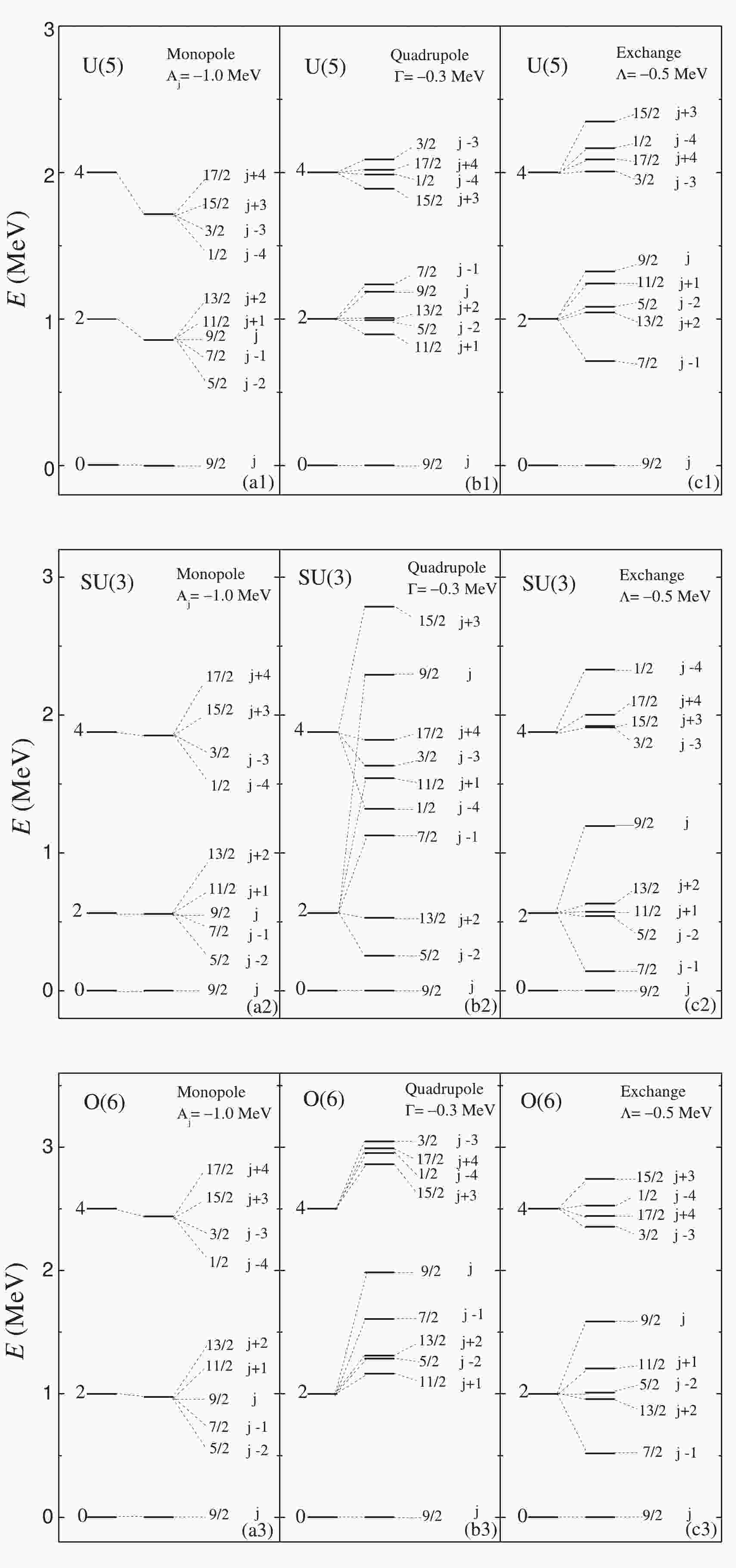
 (\epsilon_d = 1.0,\; \kappa = 0) for the U(5) limit, (\epsilon_d = 0, \; \kappa = -1/4,\; \chi = -\sqrt{7}/2) for the SU(3) limit and (\epsilon_d = 0, \; \kappa = -1/4,\; \chi = 0) for the O(6) limit. In the IBFM calculations, the three boson-fermion interactional terms defined in Eqs. (8)-(11) are individually added to the IBM Hamiltonian (4) with the adopted parameters shown in Fig. 1, where the level patterns calculated for j = 9/2 and N = 10 are shown for different scenarios. In addition, the parameter \chi involved in the quadrupole term (9) is set as \chi = -\sqrt{7}/2 for SU(3) and \chi = 0 for both O(6) and U(5) to be consistent with the consistent-Q Hamiltonian. As shown in Fig. 1(a1)-(a3), the results indicate that the level degeneracies may exactly occur for the states with |j-L|\leqslant J\leqslant j+L in the IBFM if only the monopole term is considered and the associated level pattern in each scenario is very similar to the corresponding IBM one. Thus, if no boson-fermion interactions are involved, the exact degeneracies will also occur for the states with |j-L|\leqslant J\leqslant j+L ; meanwhile, the level energies will be exactly equivalent to the corresponding values in the IBM. This means that the monopole term may only cause a renormalization of the boson level energies in each symmetry limit [40]. In contrast, if only the quadrupole term is involved, as shown in Fig. 1(b1)-(b3), the levels with different J values are not degenerated anymore. Notably, the quadrupole term at a particular strength can cause the level energy splitting in the SU(3) limit to be significantly larger than in the U(5) or O(6) limit. As further shown in Fig. 1(c1)-(c3), the exchange term can also break the level degeneracies, but with the level order in each scenario being different from the one caused by the quadrupole term. Generally, the three types of boson-fermion interactions should all be considered to obtain quantitatively good descriptions of the experimental data [45, 48].

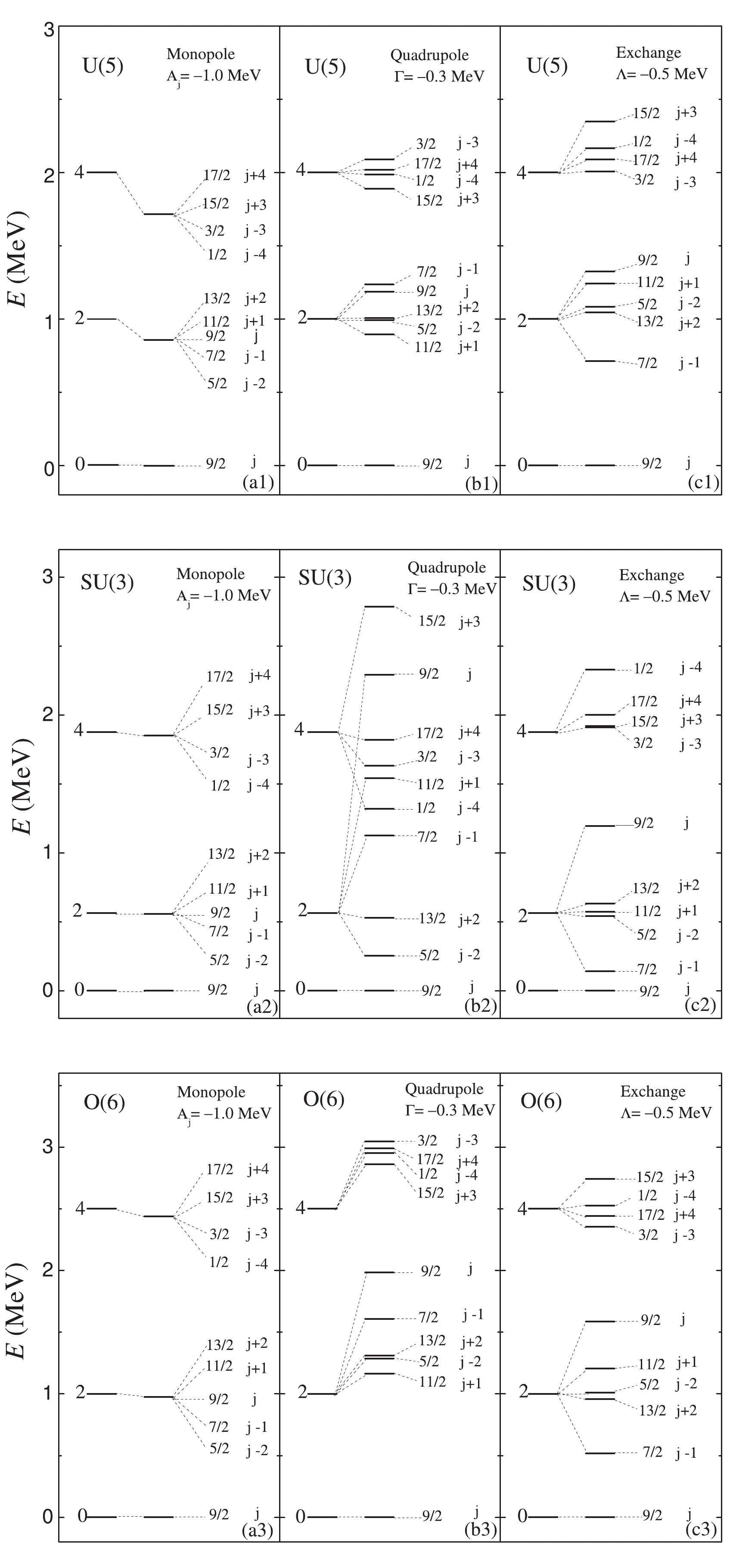
      Figure 1.  Lowest levels with L = 0,\; 2,\; 4 in the U(5), SU(3), and O(6) limits of the IBM to compare the lowest-lying levels with J = 1/2-17/2 in the IBFM, in which the results are solved using the three boson-fermion interactional terms being individually added to each symmetry limit. In the calculations, j = 9/2 and N = 10.

    III.   EFFECTS OF THE ODD PARTICLE ON SPTs

      A.   Shape phase diagram

    • The SPTs in even-even systems can be illustrated as the QPTs in the IBM. The mean-field analysis indicates that the emergence of an additional odd particle in odd-even systems can cause alternative effects on the SPTs [23-25, 34]. To examine the effects of the odd particle, it is convenient to use the consistent-Q IBFM Hamitonian:

      \hat{H}_{\mathrm{BF}} = \varepsilon \left[ (1-\eta)\hat{n}_{d} - \frac{\eta}{4N}\hat{Q}_{\mathrm{BF}}\cdot \hat{Q}_{\mathrm{BF}} \right] \, ,

      (21)

      where

      \hat{Q}_{\mathrm{BF}} \equiv \hat{Q}_\mathrm{B}^\chi+\hat{q}_\mathrm{F}\,

      (22)

      is the quadrupole operator. Compared with Eq. (9), we can derive the strength of the quadrupole boson-fermion interaction in the Hamiltonian (21) as

      \Gamma = -\frac{\varepsilon\eta}{2N}\, .

      (23)

      To calculate the B(E2) transitional rates and quadrupole moments, we can select the transitional operator as the quadrupole operator defined in (22). For simplicity, we only use the boson part; subsequently, the transitional operator is expressed as

      \hat{T}^{E2} = e\hat{Q}_\mathrm{B}^\chi\,

      (24)

      where e represents the effective charge. In practice, such an approximation closely agrees with the analysis of some deformed odd-mass nuclei using the microscopic core-quasiparticle coupling model [35]. Accordingly, the B(E2) transitional rates and quadrupole moments can be calculated via the formulas

      B(E2;J_i\rightarrow J_f) = \frac{\mid\langle J_f\parallel \hat{T}^{E2}\parallel J_i\rangle\mid^2}{2J_i+1}\,

      (25)

      and

      Q(J) = \langle JM_J = J\mid\sqrt{\frac{16\pi}{5}}\hat{T}^{E2}\mid JM_J = J \rangle\, .

      (26)

      We observed that the consistent-Q Hamiltonian above is as same as that adopted in the classical analysis in [34], which primarily focuses on the quadrupole boson-fermion interaction. This means that some predictions of the classical analysis based on the same Hamiltonian [34] can be checked in this quantal analysis.

      First, we focus on the boson core dynamics by removing the fermion term \hat{q}_F in the quadrupole operator (22). The IBFM consistent-Q Hamiltonian (21) is then reduced back to the IBM consistent-Q Hamiltonian:

      \hat{H}_{\mathrm{B}} = \varepsilon \left[ (1-\eta)\hat{n}_{d} - \frac{\eta}{4N}\hat{Q}_{\mathrm{B}}\cdot \hat{Q}_{\mathrm{B}} \right] \, ,

      (27)

      which is as same as the one in (4) but with the parameters rewritten as

      \varepsilon_d = \varepsilon(1-\eta),\; \; \kappa = -\varepsilon\frac{\eta}{4N}\, .

      (28)

      In discussions, the scale parameter is frequently set to \varepsilon = 1.0 . The IBM phase diagram in terms of the parameters in Eq. (27) can be mapped onto the Casten triangle, as shown in Fig. 2. The figure shows that each vertex of the triangle represents a particular DS, i.e., U(5) at (\eta,\chi) = (0,0) , O(6) at (\eta,\chi) = (1,0) , and SU(3) at (\eta,\chi) = \left(1,-\dfrac{\sqrt{7}}{2}\right). As mentioned earlier, these DSs are alternatively associated with different collective modes or collective shapes (deformations). Accordingly, the transitions between different collective shapes are mapped into the QPTs between different DSs and vice versa. Note that the single group, G, in the IBM phase diagram shown in Fig. 2 should be replaced with the direct product group {G}\otimes {U}(2j+1) for the IBFM [40], but we maintain the symbol G to indicate the related scenarios in both IBM and IBFM for convenience.

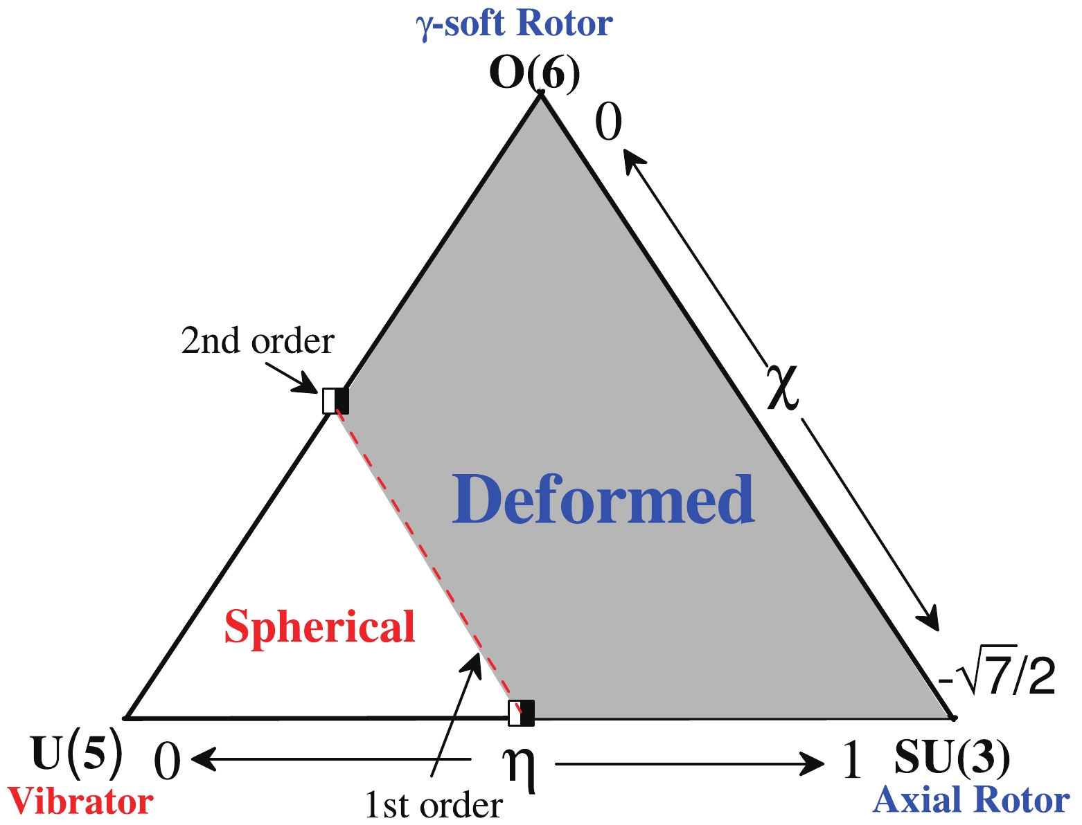
      Figure 2.  (color online) Shape phase diagram in the IBM described by the Hamiltonian (27). The dashed line denoting the 1st-order transitional points described by (29) cuts the triangle phase diagram into the spherical and deformed regions.

      Based on the mean-field analysis [14], we can prove that the system in the large-N limit experiences a 1st-order QPT at \eta_c = 8/17\simeq0.5 on the U(5)-SU(3) leg and a second-order QPT at \eta_c = 0.5 on the U(5)-O(6) leg. The U(5)-SU(3) QPT may correspond to the spherical to prolate (or the vibrator to axial rotor) SPT in the collective model terminology while the U(5)-O(6) QPT corresponds to the spherical to \gamma -soft (or the vibrator to \gamma -soft rotor) SPT. In this paper, the terminology of QPTs of the two models are mutually used without distinction. More generally, the first-order spherical to deformed SPTs (the U(5)-SU(3) QPT-like) may widely occur inside the triangle phase diagram with the critical points, expressed as

      \eta_c = \frac{14}{28+\chi^2}\, .

      (29)

      In the following, we apply the scenarios with j = 9/2 and N = 10 to discuss the effects of an odd particle on the U(5)-SU(3) and U(5)-O(6) SPTs in the finite systems. In particular, we compare the results solved from the IBFM Hamiltonian (21) to those obtained from the IBM Hamiltonian (27). Note that the effects of different boson-fermion interactions on the spectra in the two types of SPTs have been previously investigated in the IBFM both classically and quantum mechanically [26]. In the following, we focus on revealing the similarities and differences in the critical behaviors of the odd-even and even-even systems.

    • B.   Finite-N critical features

    • First, the lowest-lying levels are computed, and the results evolving as functions of \eta in both the U(5)-SU(3) and U(5)-O(6) transitional regions are shown in Fig. 3. As shown in Fig. 3(a), the states with different J values in the odd-even systems are approximately degenerate and are divided into groups with the level energies being close to those with L = 0,\; 2,\; 4 in the even-even system until \eta\sim0.4 ; subsequently, the degeneracies are rapidly broken in the range of \eta\sim0.4-0.6 with the levels reorganized in a spread. This is the finite precursor of the U(5)-SU(3) SPT in odd-even systems. Note that an SPT in a finite system may occur in a parameter region rather than at a point owing to the finite-N effect, which also results in the transitional features not being as sharp as that in the large-N limit [14], where the concept of QPT is rigorously defined. As further shown in Fig. 3(b), the level degeneracies in the odd-even systems clearly break down in the critical region \eta\sim0.4-0.6 , which confirms that the U(5)-O(6) SPT also occurs in the odd-even systems. In theory, the breaking of level degeneracies can be considered to be a signal for U(5)-O(6) SPT. Meanwhile, the results imply that the transitional features of the second-order QPT (U(5)-O(6) SPT) in a finite-N system may be significantly weaker than those of the first-order QPT (U(5)-SU(3) SPT).

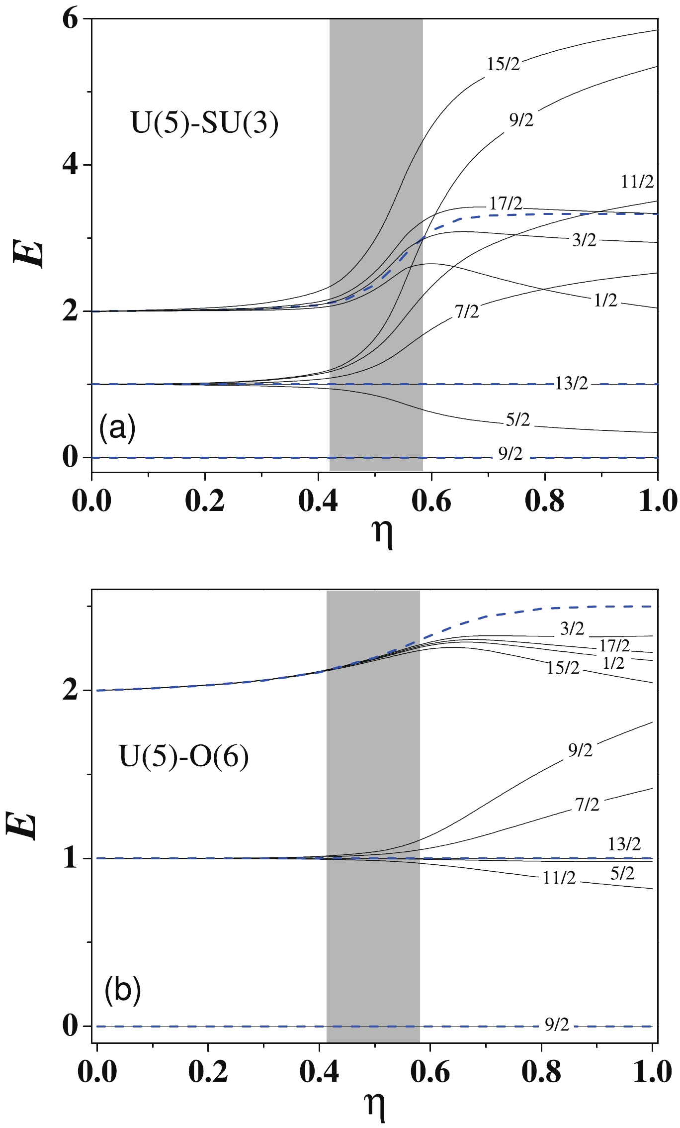
      Figure 3.  (color online) Low-lying energy levels evolving as functions of the control parameter \eta in both the U(5)-SU(3) and U(5)-O(6) transitions; the grey color indicates the critical region in a finite-N scenario. In the calculated results, the levels with L = 0,\; 2,\; 4 in the IBM (denoted by dashed lines) have been normalized to E(2_1) = 1.0 and those with J = 1/2-17/2 in the IBFM (denoted by full lines) are normalized to E(13/2_1) = 1.0.

      To further identify the critical features in a finite-N situation, the energy ratio R_{4/2} and the B(E2) ratio B_{4/2} are calculated for the two types of SPTs with the corresponding results as a function of \eta shown in Fig. 4 and Fig. 5, respectively. As shown in Fig. 4(a), a sudden increase in R_{4/2} can be observed in the critical region of the U(5)-SU(3) SPT, which confirms again that this type of SPT indeed occurs in the odd-even system as in the adjacent even-even system. An interesting observation is that the transitional feature in R_{4/2} seems to be slightly enhanced in the odd-even system. In contrast, the results shown in Fig. 4(b) indicate that the finite-N precursor of U(5)-O(6) SPT can be also identified from the evolutions of R_{4/2} but with the transitional amplitude in the odd-even system ( R_{4/2}\sim2.0-2.3 ) being more depressed than in the adjacent even-even system ( R_{4/2}\sim2.0-2.5 ). This means that the U(5)-O(6) SPT may be smoother in the odd-even nuclei owing to the effects of the odd particle, which agrees with the classical analysis provided in [34]. As shown in Fig. 5, the results for the B(E2) ratio further confirm the finite-N precursors of the SPTs in the odd-even and even-even systems. The figure shows that the U(5)-SU(3) transitional features are strengthened by the effects of the odd particle, and the transitional amplitude of B_{4/2} in the odd-even system is relatively larger than that in the even-even system. In contrast, the U(5)-O(6) SPT features in the odd-even system become relatively weaker with a smaller amplitude of B_{4/2} than in the adjacent even-even systems. Reference [49] indicated that ratio B_{4/2} in the even-even system can be applied as the effective order parameter to distinguish the first-order SPT (U(5)-SU(3)) from the second-order SPT (U(5)-O(6)) by its different evolutional characteristics in the two types of SPTs. We can observe in Fig. 5 that B_{4/2} in the odd-even system can have the same function as the differences in between the first-order and second-order SPTs become even larger owing to the effects of the odd particle.

      Figure 4.  (color online) Typical energy ratios evolving as functions of \eta in the U(5)-SU(3) and U(5)-O(6) SPTs with the definition R_{4/2}\equiv \frac{E((4+J_g)_1)}{E((2+J_g)_1)}, where the ground state spins J_g = 9/2 and J_g = 0 are used in the calculations for the odd-even and even-even systems, respectively.

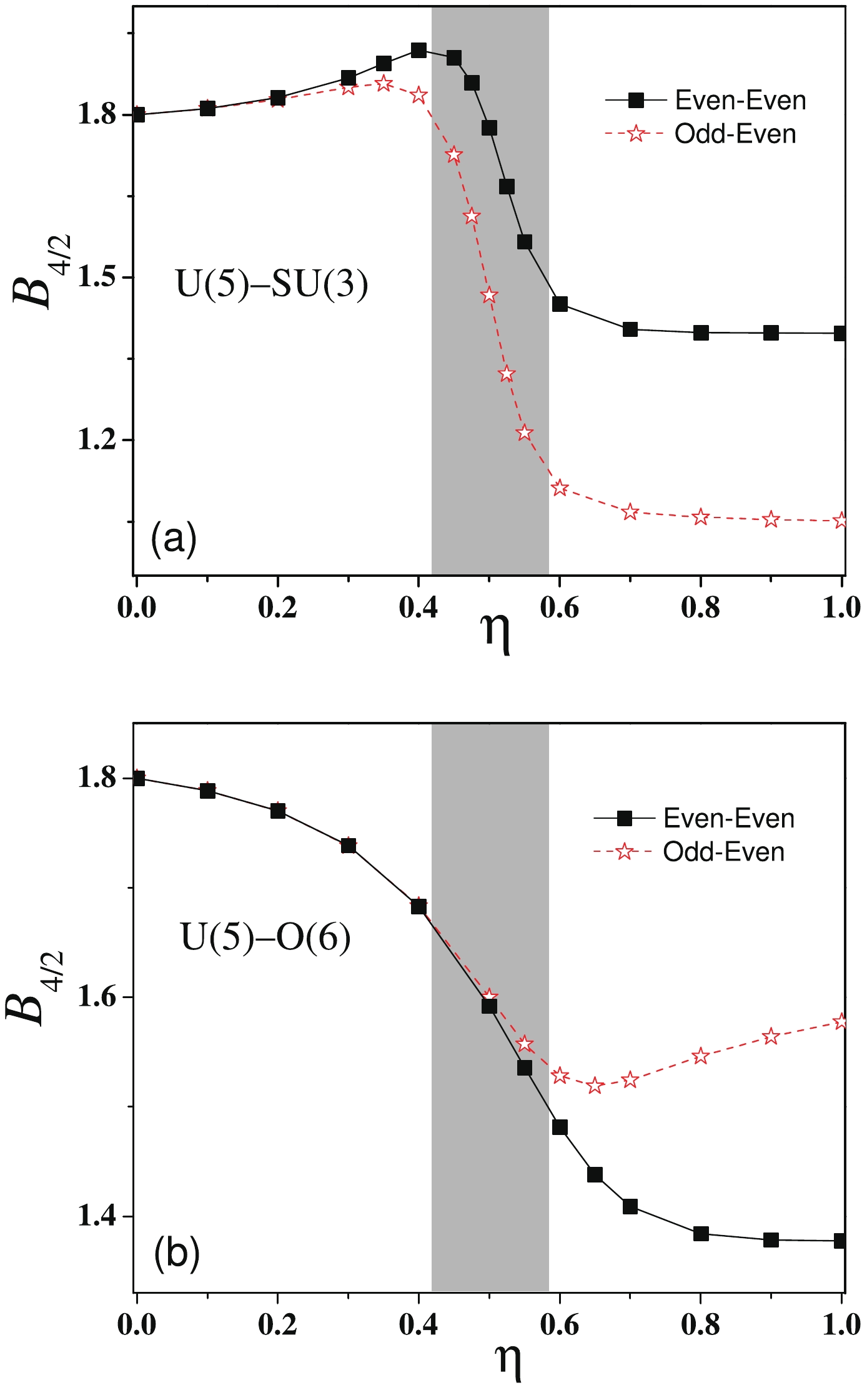
      Figure 5.  (color online) Same as in Fig. 4 but for the B(E2) ratios defined as B_{4/2}\equiv\frac{ B(E2;(4+J_g)_1\rightarrow(2+J_g)_1)}{B(E2;(2+J_g)_1\rightarrow(0+J_g)_1)} with J_g = 9/2 and J_g = 0 used for the odd-even and even-even systems, respectively.

      To check the deformations of the finite systems in the SPTs, the quadrupole moments of the even-even system, Q(2_1) , and those of the odd-even system, Q(J_1) , have been calculated, and the results as a function of \eta are shown in Fig. 6. As shown in Fig. 6(a), the quadrupole moments of the selected states in the U(5)-SU(3) transition may all decrease from the nearly zero values to the negative values with the fastest change appearing in \eta = 0.4\sim0.6 as expected. A noticeable scenario is that Q(7/2_1) as a function of \eta may gradually increase until \eta\sim0.4 before beginning to decrease. A more interesting observation from the sub-panel is that the odd-even differences \Delta Q for the different states nearly all attain their maxima in the critical region, which indicates that the odd particle can induce a larger fluctuation in the quadrupole deformation in the critical systems. This implies that different deformations (phases) may have more opportunities to coexist in the low-lying structures of the odd-even systems undergoing the U(5)-SU(3) SPT [34]. For the U(5)-O(6) SPT, we can observe from Fig. 6(b) that the quadrupole moments of the even-even system, Q(2_1) , remains zero in the entire transitional process. It is easy to understand this feature from the selection rule as the transitional operator \hat{Q}_\mathrm{B}^{\chi = 0} adopted in the calculation for the U(5)-O(6) SPT requires \Delta L = \pm2 for the yrast states [15]. In contrast, the quadrupole moments of the odd-even system, Q(J_1) , may all monotonically decrease from zero to the negative values, thus suggesting that the largest odd-even difference of quadrupole deformation in the U(5)-O(6) SPT should appear in the O(6) limit. In addition, the results in Fig. 6(a) are not exactly equivalent to zero for the U(5) limit. This is primarily because of a different transitional operator, \hat{Q}_\mathrm{B}^{\chi = -\frac{\sqrt{7}}{2}} , being selected for the U(5)-SU(3) SPT to be consistent with the consistent-Q Hamiltonian; however, this observation will not change the conclusions.

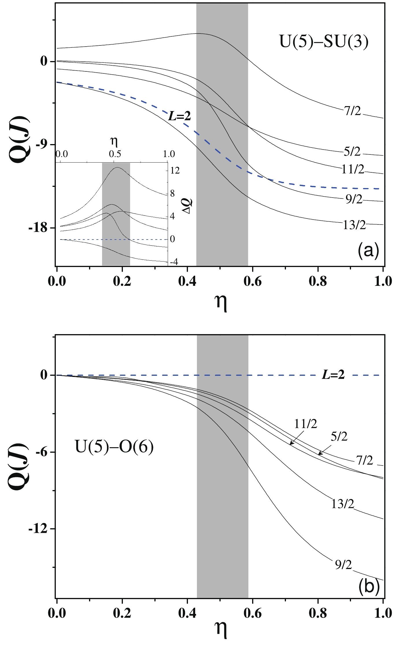
      Figure 6.  (color online) Quadrupole moments, Q(J), evolving as functions of \eta in the two types SPTs. The dashed lines represent the results for the 2_1 state in the even-even system, and the full lines represent the lowest states with \mid j-2\mid\leq J\leq j+2 in the odd-even system. In the calculations, the effective charge in the transitional operator (24) has been set to e = 1.0. The sub-panel shows the odd-even differences of the quadrupole moments defined as \Delta Q = Q(J_1)-Q(2_1).

      Finally, we discuss the one-particle-transfer spectroscopic intensities for stripping and pick-up reactions. In leading order, the spectroscopic intensities in the IBFM are described by the square of the one-fermion addition and removal matrix elements [40]. Specifically, we consider the transfer process by adding the even-even system with a j = 9/2 fermion to the even-even system or removing a j = 9/2 fermion from the odd-even system. The corresponding spectroscopic intensities can be calculated using

      I(\mathrm{Even}\rightarrow \mathrm{Odd}) = e_\alpha^2\mid\langle\alpha_fJ_f\parallel a_{9/2}^\dagger\parallel\alpha_iL_i\rangle\mid^2\,

      (30)

      and

      I(\mathrm{Odd}\rightarrow \mathrm{Even}) = {e_\alpha^\prime}^2\mid\langle\alpha_f^\prime L_f^\prime\parallel \tilde{a}_{9/2}\parallel\alpha_i^\prime J_i^\prime\rangle\mid^2\,

      (31)

      where e_\alpha (e_\alpha^\prime) represents the scale parameter. Clearly, the one-particle-transfer processes can provide a direct connection between the odd-even and even-even systems in a particular SPT.

      The evolution of one-particle-transfer spectroscopic intensities as a possible signature of the U(5)-O(6) SPT was previously investigated for j = 3/2 [19]. Here, we compare the critical features of the spectroscopic intensities in between the U(5)-O(6) and U(5)-SU(3) SPTs. To accomplish this, the calculated results for I(0_1\rightarrow9/2_1) , I(0_1\rightarrow9/2_2) , I(9/2_1\rightarrow0_1) and I(9/2_1\rightarrow2_1) as functions of \eta are shown in Fig. 7. Fig. 7(a) shows that the intensities for the pick-up reactions, I(\mathrm{Even}\rightarrow \mathrm{Odd}) , may rapidly either increase or decrease in the critical regions for both the U(5)-SU(3) and U(5)-O(6) SPT but with the transitional signatures in the former being clearly stronger than in the latter. A very similar scenario can be observed in the spectroscopic intensities for stripping reactions, I(\mathrm{Odd}\rightarrow \mathrm{Even}) , as shown from Fig. 7(b). The results indicate that the evolutions of one-particle-transfer spectroscopic intensities can provide alternative signatures of the SPTs, particularly for the U(5)-SU(3) transition, in addition to those typically used energies and electromagnetic observables.

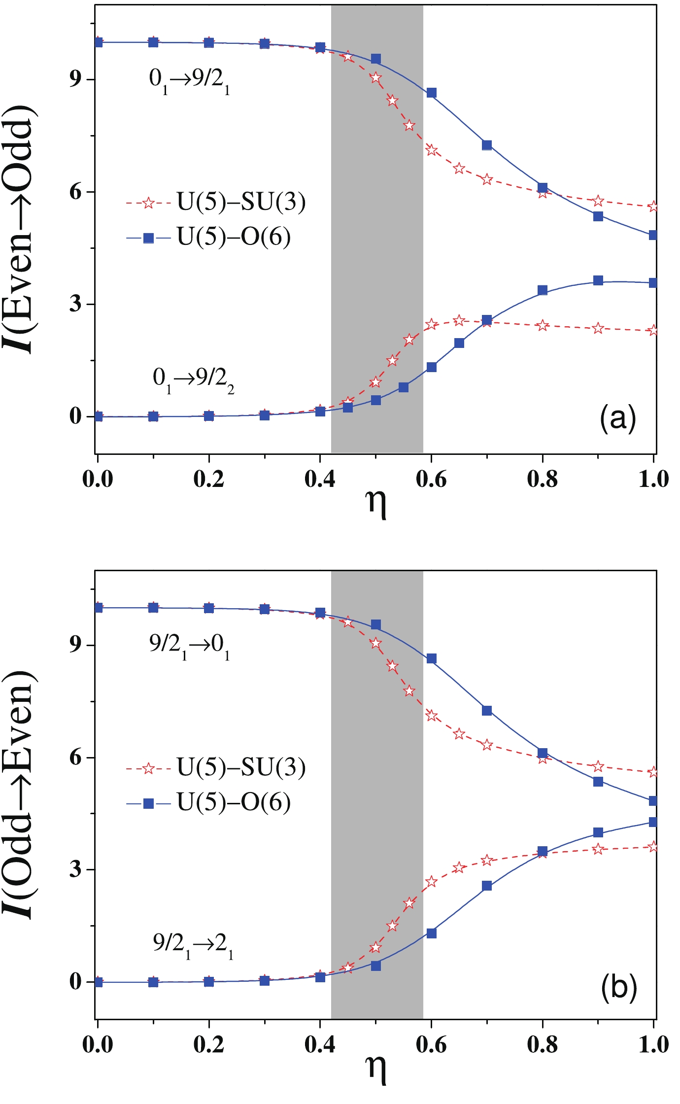
      Figure 7.  (color online) Typical one-particle-transfer spectroscopic intensities evolving as functions of \eta in the two types of SPTs. In the calculations, the scale parameters have been set to e_\alpha = e_\alpha^\prime = 1.0.

    IV.   SUMMARY
    • A scheme of diagonalizing the IBFM Hamiltonian in terms of the SU(3) coupling basis has been introduced, through which a quantal analysis of the effect of the odd particle on two types of SPTs is performed in the IBFM by comparing the critical behaviors of some select observables. Similar to the even-even systems, we demonstrate that the U(5)-SU(3) and U(5)-O(6) SPTs can also occur in the odd-even system. More importantly, the results indicate that the effects of the odd particle may further strengthen the U(5)-SU(3) transitional features but weaken the U(5)-O(6) ones. This observation closely agrees with the previously classical analysis [24, 25, 34] of the two types of SPTs, thus providing observable proofs of the mean-field predictions. Furthermore, we reveal that the fluctuations of the quadrupole deformations in the odd-even systems become larger when approaching the critical point of the U(5)-SU(3) SPT, which implies the potential for phase coexistence in the critical odd-A nuclei. The paper presents a schematic illustration of the actual scenarios for odd-A nuclei, as the discussions are confined to scenarios with the odd particle being assumed to move in a single j shell. Multi-particle (-hole) in multi-j scenarios may require to be considered for a more general representation, particulalry for searching for the potential phase coexistence in experiments [28]. In addition to the two types of transitions discussed herein, the effects of an odd particle on other types of SPTs (such as the prolate to oblate transition) remain to be studied [16]. Related research is in progress.

Reference (49)

目录

/

DownLoad:  Full-Size Img  PowerPoint
Return
Return