


 Abstract
 HTML
HTML Reference
 Related
 PDF
PDF


-
The dark matter (DM) is an unsolved puzzle in cosmology and particle physics, and it probably consists of particles that are weakly interacting. Though many astronomical observations, like Cosmic Microwave Background and baryon acoustic oscillations, approximately DM make up 23% of today's Universe. The cosmological model based on cold DM in reproducing the large-scale structure of the Universe is quite well and get great success [1-7]. The most popular candidate for cold DM is the weakly interacting massive particles (WIMPs), which are particles with negligible self-interactions, they are stable and collisionless. Their particle masses estimated are in the range 10 GeV ~ 1 TeV.
However, several severe challenges to the cold dark matter model have emerged on a small scale, such as the scale of individual galaxies and their central core [2]. For example, in the cold DM model, halos can be characterized by a power-law mass density distribution with a steep power index at the central core, which is in contrast with the observation in small scale, such as the observed rotation curves of low surface brightness (LSB) galaxies. This indicates the existence of a central constant-density DM core [8] in LSB galaxies, which comprise a very small proportion of ordinary baryonic matter, such that their stellar populations make only a relatively small contribution to the observed rotation curves. The rotation curves of galaxies are important observational tools in detecting their gravitational potential. Because the luminous component cannot fit the entire rotation curve of galaxies, it requires a contribution by dark matter or other ideas, such as modified Newtonian dynamics (MOND) [9, 10]. When we use dark matter to explain the observed rotation curves of galaxies, several empirically spherical dark matter halo profiles exist [11], such as the Navarro-Frenk-White (NFW) [12], Burkert [13] and pseudo-isothermal profiles [14]. The Burkert and pseudo-isothermal profiles are often used for LSB galaxies, and they can perfectly fit the observed rotation curves of LSB galaxies [15-17]. They both indicate the existence of a central constant density. However, by adopting the cold DM model, numerical N-body simulations cannot reproduce a central constant-density DM core [18]. This phenomenon is called the cusp-core problem.
Furthermore, LSB galaxies are valuable laboratories for the indirect detection of DM [19]. They are late-type disc galaxies with a face-on central surface brightness fainter than that of the night sky. It is very difficult to detect them owing to their very low surface brightness. LSB galaxies are the most abundant objects in the Universe, and they possibly contribute
$ \gtrsim $ 50% to the galaxy population [17, 20]. In addition, they are generally isolated systems [21]. The pair annihilation of WIMPs can produce high energy$ \gamma $ -rays [22]. Star formation, accreting supermassive black holes, or active galactic nuclei (AGN) can also trigger$ \gamma $ -ray emission. LSB galaxies generally have very low star formation rates, and are characterized by diffuse, metal poor, and very low surface density exponential stellar discs. They are slowly evolving galaxies. AGNs are rarely discovered in LSB galaxies [23]. Moreover, LSB galaxies are very rich in neutral hydrogen ($ {\rm H_{I}} $ ) gas. On average, the masses of$ {\rm H_{I}} $ gas in their gas discs range from$ 10^{8} $ to$ 10^{10} M_{\odot} $ [24]. The extended gas discs can extend outward to approximately 2-3 times their stellar disks [25, 26]. This enables us to measure their rotation curves to large radii by adopting the$ {\rm H_{I}} $ data. Their rotation curves can also be derived from the other emission lines such as the$ {\rm H_{\alpha}} $ line [15, 27, 28]. Rotation curve studies demonstrate that LSB galaxies are significantly dominated by DM and have simple a dynamical structure.Other popular DM models are used to explain the cusp-core problem, such as the self-interacting DM [29] and warm dark matter model (WDM) [30, 31]. Two of the most canonical candidates for WDM are the sterile neutrino [32] and the gravitino [33]. The dark matter particles are usually classified by their velocity dispersion given in terms of three broad categories: hot DM (HDM), warm DM (WDM) and cold DM (CDM). In principle, HDM is relativistic at all cosmological relevant scales. When a particle's momentum is equal to or less than its mass, it becomes non-relativistic. The WDM has a higher velocity than the CDM because of their mass. The typical mass of the WDM particle is approximateky 1 keV. On subgalactic and galactic scales, their non-zero thermal velocities have a substantial suppression effect on the steep DM power spectrum [31].
In this study, we attempt to investigate the equation of state of DM to elucidate the cusp-core problem. Based on the nature of WDM, we hypothesize that DM has a nonzero random motion in the density core. However, when DM is a perfect fluid, the observations indicae that the velocity of this random motion is significantly lesser than the speed of light. In reality, this constant random motion probably disappears at large radii; hence, this term can be replaced by the polytropic model. Considering the properties of WIMPs, we can assume that the random motion of dark matter particles is positively correlated with their rotational motions at large scale. Moreover, because several halo density profiles, such as the NFW profile or pseudo-isothermal profile, can be effectively used to fit the density profile of the galaxies from small sizes to large sizes, we can assume that the equation of state is independent of the scaling transformation. In this study, we will demonstrate that its lower order approximation for this type of equation of state can naturally yield a result in which the random motion of dark matter include a constant term, including a term that is proportional to the particle rotational motions. In this simple phenomenological model, we can observe that the dark matter halo profile agrees well with the observations. It can provide a solution for the cusp-core problem.
The outline of this paper is as follows. In Section II, we present three special cases for the equation of state of DM and obtain the mass density profiles of DM halos. We obtain an approximate analysis to describe the interactive effect between DM and black hole in Subsection II.A. In subsection II.B, we study the aforementioned phenomenological model and compare it with the observations. In subsection II.C, to enable the constant random motions disappear at large radii, this term is replaced by the polytropic model. We then study this novel model. In Section III, we present the conclusions of this study.
-
The most general static and spherically symmetric metric takes the following form
$ {\rm d}s^{2} = {\rm e}^{A}{\rm d}t^{2}-{\rm e}^{B}{\rm d}r^{2}-r^{2}({\rm d}\theta^{2}+\sin^{2}{\theta}{\rm d}\phi^{2}), $

(1) where A and B are functions of r. For conventions, the gravitational constant and speed of light are set to 1. Using the above metric, the Einstein gravitational field equation can be expressed as follows.
$ \begin{aligned}[b]&-{\rm e}^{-B}\left(\frac{1}{r^{2}}-\frac{B_{r}^{\prime}}{r}\right)+\frac{1}{r^{2}} = 8\pi T_{t}^{t}, \\& -{\rm e}^{-B}\left(\frac{1}{r^{2}}+\frac{A_{r}^{\prime}}{r}\right)+\frac{1}{r^{2}} = 8\pi T_{r}^{r}, \\& \frac{-{\rm e}^{-B}}{2}\left[A_{rr}^{\prime\prime}+\frac{(A_{r}^{\prime})^{2}}{2}+\frac{A_{r}^{\prime}-B_{r}^{\prime}}{r}-\frac{A_{r}^{\prime}B_{r}^{\prime}}{2}\right] = 8\pi T_{\theta}^{\theta} = 8\pi T_{\phi}^{\phi}. \end{aligned} $

(2) By analyzing the stable circular orbits of a test particle, the rotation velocity
$ V_{\rm rot} $ of a test particle can be expressed as [34, 35]:$ V_{\rm rot}^{2} = \frac{1}{2}rA_{r}^{\prime}. $

(3) If pure DM is an isotropic perfect fluid, its energy momentum tensor takes the form
$ T^{\mu}_{\nu} = {\rm diag}[\rho, $ $ -p, -p, -p] $ for the spherically symmetric case. Let us set$ F = {\rm e}^{-B}-1 $ ,$ N = A_{x}^{\prime} $ , and$ x = \ln(r) $ . Then Eq. (2) becomes$ F+F_{x}^{\prime}+8\pi r^{2}\rho = 0, $

(4) $ (1+F)N+F = 8\pi r^{2}p, $

(5) $ (1+F)\left[N_{x}^{\prime}+\frac{1}{2}N^{2}\right]+\frac{1}{2}F_{x}^{\prime}N+F_{x}^{\prime} = 16\pi r^{2} p. $

(6) It yields
$ \frac{{\rm d}p}{{\rm d}x} = -\frac{p+\rho}{2}N. $

(7) This equation can lead to
$ \dfrac{{\rm d}p}{{\rm d}r} = -\rho g $ in a non-relativistic approximation, where g is the gravity acceleration. Then, in a relativistic case, we have the following equation:$ N_{x}^{\prime}+\left[\frac{F_{x}^{\prime}}{2(1+F)}-2\right]N+\frac{N^{2}}{2}+\frac{F_{x}^{\prime}-2F}{1+F} = 0. $

(8) To solve this equation, we need the equation of state (EOS). Because combining Eqs. (4) and (5) yields the following expression
$ \frac{p}{\rho} = -\frac{(1+F)N+F}{F+F_{x}^{\prime}}, $

(9) assuming that pressure p is the only the function of density
$ \rho $ , N is a function of$ x, F_{x}^{\prime} $ and F, and it is expressed as$ N = G(x,F,F_{x}^{\prime}) $ . If$ F(r) $ is a solution and$ \lambda $ is a positive constant, then$ F(\lambda r) $ is also its solution. This assumption leads to the equation$ N = G $ obviously does not contain x, as it is an autonomous equation. However, this also leads to pressure p being proportional to density$ \rho $ . To consider more possible EOS, we just assume that N is a function of$ F_{x}^{\prime} $ and F. The rotation velocity is significantly less than the speed of light; hence, F is negligible. When F and$ F_{x}^{\prime} $ are negligible, we can adopt the Taylor expansion of equation$ G(F,F_{x}^{\prime}) $ to replace them. Because Eq. (9) can be solved by iteration,$ \begin{aligned}[b]&N_{0} = -F, \\ &N_{1} = -F\left(1+\dfrac{3F_{x}^{\prime}-5F-F^{2}}{4+4F-F_{x}^{\prime}}\right)\approx -F\left(1+\frac{3}{4}F_{x}^{\prime}-\frac{5}{4}F\right),\\& N_{2}\approx -F\left(1-\dfrac{1}{2}F_{x}^{\prime}-\dfrac{5}{4}F+\dfrac{3}{8}F_{xx}^{\prime\prime}\right)-\dfrac{3}{8}(F_{x}^{\prime})^{2}, \\ & ... \end{aligned} $

(10) Considering the above approximate iteration form of variable N, we take two cases of the Taylor expansion of the equation
$ N = G(F,F_{x}^{\prime}) $ to solve Eq. (9) in the following Subsections II.A and II.B. We then consider an extended EOS of dark matter in subsection II.C. This EOS is not an autonomous equation. -
Using the first iteration formula
$ N_{1} $ , we can assume$ N = -F+(\gamma F+\epsilon F_{x}^{\prime})F, $

(11) where
$ \gamma $ and$ \epsilon $ are constant. When$ |F|\ll 1 $ and$ |F_{x}^{\prime}|\ll 1 $ , using Eqs. (3)-(5), this assumption leads to the following EOS:$\begin{aligned}[b] p =& \frac{(1+F)N+F}{8\pi r^{2}}\approx\frac{\epsilon(F_{x}^{\prime}+F)F+(\gamma-\epsilon-1)F^{2}}{8\pi r^{2}}\\\approx& 2\epsilon V_{\rm rot}^{2}\rho+\frac{\gamma-\epsilon-1}{2\pi}\left(\frac{V_{\rm rot}^{2}}{r}\right)^{2}. \end{aligned} $

(12) When
$ |F|\ll 1 $ and$ |F_{x}^{\prime}|\ll 1 $ , and setting$ M = \ln(-F) $ , Eqs. (9) and (12) can be approximated by$ 2\epsilon U_{x}^{\prime}+(4\gamma-4\epsilon-3)U+4\epsilon U^{2}+5-4\gamma = 0, $

(13) where
$ U = M_{x}^{\prime} $ . This equation is a Riccati equation. When$ (4\gamma+4\epsilon-3)^{2}-32\epsilon >0 $ , one of the solutions is$ F = -\frac{b}{r^{\widetilde{\alpha}}}\sqrt{ 1+\left(\frac{r}{r_{0}}\right)^{\widetilde{\beta}}}, \;\;\;\; ( \widetilde{\beta} > 0), $

(14) where
$ \widetilde{\alpha} = \dfrac{4\gamma-4\epsilon-3}{8\epsilon}+\dfrac{\widetilde{\beta}}{4} $ ,$ \widetilde{\beta} = \dfrac{\sqrt{(4\gamma+4\epsilon-3)^{2}-32\epsilon}}{2|\epsilon|} $ , b and the core radius$ r_{0} $ are positive constants. Then the density$ \rho $ is$ \rho = -\frac{F}{8\pi r^{2}}\left[1-\widetilde{\alpha} +\frac{\widetilde{\beta}\left(\dfrac{r}{r_{0}}\right)^{\widetilde{\beta}}}{2+2\left(\dfrac{r}{r_{0}}\right)^{\widetilde{\beta}}}\right]. $

(15) If density is characterized by a power-law distribution
$ \rho \sim r^{\alpha} $ , using Eq. (4),$ \alpha $ can be written as$ \alpha = \frac{r\rho_{r}^{\prime}}{\rho} = \frac{F_{x}^{\prime}+F_{xx}^{\prime\prime}}{F+F_{x}^{\prime}}-2. $

(16) The absolute value of the slope
$ \alpha $ should be higher in the outer region. Considering the fact that DM density$ \rho $ has a lower value and its absolute value of slope$ \alpha $ is higher in the outer region,$ \widetilde{\alpha} $ should be equal to 1. This leads to$ \gamma = 1+\epsilon $ , then it is easy to observe that p is proportional to the term$ V_{\rm rot}^{2}\rho $ , i.e.$ p\approx 2\epsilon V_{\rm rot}^{2}\rho $ (i.e.$ \dfrac{(1+F)N+F}{8\pi r^{2}} = -\epsilon N\dfrac{F_{x}^{\prime}+F}{8\pi r^{2}} $ ), and the variable N is given by$ N = - \frac{F}{1+F+\epsilon F+\epsilon F_{x}^{\prime}}. $

(17) Thus, using Eq. (9) can lead to the following equation:
$ \begin{aligned}[b] 2\epsilon F_{xx}^{\prime\prime}&+F_{x}^{\prime}\left(1-\epsilon+\frac{\epsilon-6\epsilon^{2}F}{1+F}\right) +\frac{\epsilon (F_{x}^{\prime})^{2}}{F}\left(1+\frac{1+2\epsilon F_{x}^{\prime}}{1+F}\right)\\& +(1-4\epsilon)F-\frac{4\epsilon^{2}F^{2}}{1+F} = 0, \end{aligned}$

(18) and Eq. (15) is reduced into the form
$ F = -\frac{b}{r}\sqrt{ 1+\left(\frac{r}{r_{0}}\right)^{\frac{8\epsilon-1}{2\epsilon}}}. $

(19) When the core radius
$ r_{0}\rightarrow\infty $ , this solution can become the vacuum Schwarzschild solution, and the parameter b is the Schwarzschild radius in this case. Then the energy density$ \rho $ can be approximated as$ \rho = \frac{(8\epsilon-1)b}{32\epsilon\pi r_{0}^{3}}\frac{\left(\dfrac{r}{r_{0}}\right)^{\frac{2\epsilon-1}{2\epsilon}}}{\sqrt{ 1+\left(\dfrac{r}{r_{0}}\right)^{\frac{8\epsilon-1}{2\epsilon}}}}. $

(20) This profile is a Zhao halos profile [36], which can acquire both the form of a cusped or a cored profile with three free parameters (
$ \overline{\alpha}, \overline{\beta}, \overline{\gamma} $ ):$ \rho = \frac{\rho_{0}}{\left(\dfrac{r}{r_{0}}\right)^{\overline{\gamma}}\left( 1+\left(\dfrac{r}{r_{0}}\right)^{\overline{\alpha}}\right)^{\frac{\overline{\beta}+\overline{\gamma}}{\overline{\alpha}}}}. $

(21) When
$ r_{0} $ is significantly large, a transition zone exists between the density core and outer region when density is characterized by a power-law distribution$ \rho \sim r^{\alpha} $ for the profile in Eq. (21). In this transition zone, the slope is altered from$ \alpha = \dfrac{2\epsilon-1}{2\epsilon} $ to$ \alpha = -\dfrac{1+4\epsilon}{4\epsilon} $ . For example, when$ \epsilon = 0.5 $ , the density distribution is dominated by a central constant-density core, as well as by an outer power-law density distribution$ \rho \sim r^{-1.5} $ . Because DM has lower density in the outer region, the interaction force of the DM decreases and variable$ \epsilon $ may be smaller at a larger radii; hence, we probably obtain a steeper outer power-law density distribution in this more realistic case, such as the pseudo-isothermal profile$ \dfrac{\rho_{0}}{1+(r/r_{0})^{2}} $ . Unfortunately, a severe problem exists. Because b is the Schwarzschild radius, the mass of the dark matter within the core radius is only$ \sqrt{2}-1 $ times the black hole mass. This is not consistent with the observations. The observations show that the mass of the central black hole is far less than that of the DM halo for many types of galaxies [37-39].To test the approximate analysis in Eq. (20), we adopt the odeint Python routine in the SciPy library to solve Eq. (19). Because the energy density
$ \rho $ cannot be solved easily by Eq. (2), using Eqs. (2) and (19), the energy density$ \rho $ can be rewritten as$\begin{aligned}[b] \ln(8\pi r^{2}\rho)_{x}^{\prime} =& \frac{F_{xx}^{\prime\prime}+F_{x}^{\prime}}{F_{x}^{\prime}+F} = -\frac{1}{2\epsilon}\Bigg[1-4\epsilon+\frac{\epsilon F_{x}^{\prime}}{F}\\&+\frac{\epsilon F_{x}^{\prime}}{F(1+F)}-\frac{2\epsilon^{2}F_{x}^{\prime}}{1+F} +\frac{2\epsilon^{2}(F_{x}^{\prime})^{2}}{F(1+F)}-\frac{4\epsilon^{2}F}{1+F}\Bigg].\end{aligned} $

(22) Then, using Eq. (23), we obtain the density
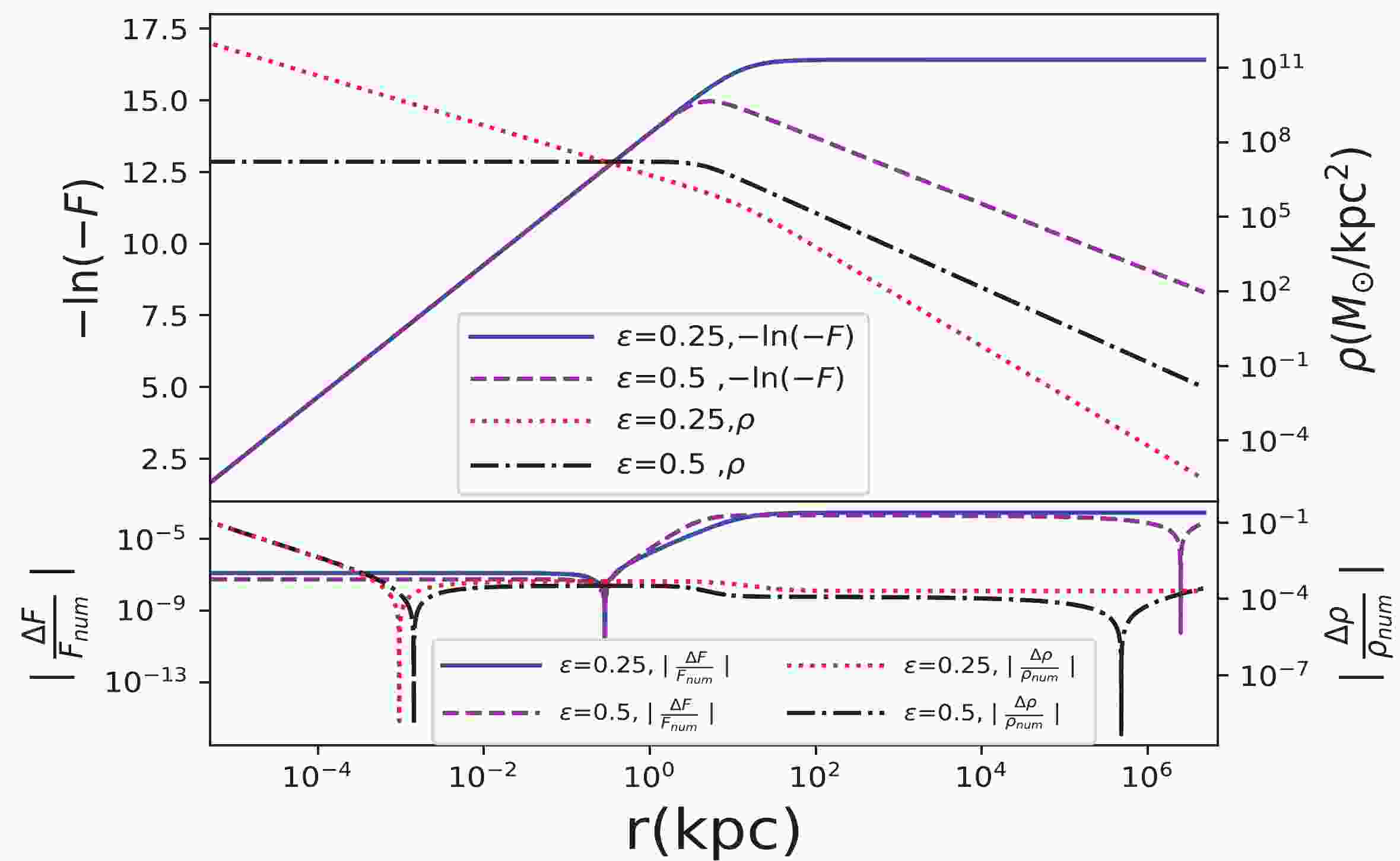
$ \rho $ . In Fig. 1, we compared our approximated analytical solutions with the full numerical solutions for F and$ \rho $ . Notably, their difference is negligible, i.e., the relative differences are generally below$ 10^{-4} $ , with most of them at$ 10^{-4}-10^{-5} $ level. The relative errors of density$ \rho $ become larger and can obtain$ 10^{-1} $ at the inner region near the black hole. The analytical solution can directly provide the density profile form.
Figure 1. (color online) Comparison results between the approximate analysis and numerical solutions. (top) The analytical solutions of
$ -\ln(-F) $ and$ \rho $ . The solid and dashed lines represent$ -\ln(-F) $ when$ \epsilon $ = 0.25 and 0.5, respectively. The dotted and dashed-dotted lines represent$ \rho $ when$ \epsilon $ = 0.25 and 0.5, respectively. (bottom) The relative errors ($\mid\dfrac{\Delta F}{F_{\rm num}}\mid = \mid\dfrac{ F_{\rm num}-F_{\rm app}}{F_{\rm num}}\mid$ and$ \mid\dfrac{\Delta \rho}{\rho_{num}}\mid = \mid\dfrac{ \rho_{\rm num}-\rho_{\rm app}}{\rho_{\rm num}}\mid $ ) for different$ \epsilon $ . The subscripts$ {\rm num} $ and$ {\rm app} $ refer to quantities relating to the numerical solutions and approximate analysis, respectively. The solid and dashed linescorrespond to$ \mid\dfrac{\Delta F}{F_{\rm num}}\mid $ when$ \epsilon $ = 0.25 and 0.5, respectively. The dotted and dashed-dotted lines give$ \mid\dfrac{\Delta \rho}{\rho_{num}}\mid $ when$ \epsilon $ = 0.25 and 0.5, respectively. -
In the previous case, the solution that satisfies the boundary conditions does not exist
$ \begin{array}{l}F = 0, \; \; \alpha\approx 0 \; \; \; {\rm at}\; \; \; r = 0 \\ \alpha\approx -2 \; \; \; {\rm at}\; \; \; r = \infty. \end{array} $

(23) Assume that
$ N = -F-\zeta(F+F_{x}^{\prime})+(1+\epsilon )F^{2}+\epsilon F_{x}^{\prime}F, $

(24) where
$ \zeta $ is a negligible positive constant [34, 40]. When$ |F|\ll 1 $ and$ |F_{x}^{\prime}|\ll 1 $ , using Eqs. (3)-(5), this assumption leads to the following EOS:$ p = \frac{(1+F)N+F}{8\pi r^{2}}\approx\frac{-\zeta(F+F_{x}^{\prime})+\epsilon(F_{x}^{\prime}+F)F}{8\pi r^{2}}\approx \zeta\rho+ 2\epsilon V_{\rm rot}^{2}\rho. $

(25) When
$ |F|\ll 1 $ and$ |F_{x}^{\prime}|\ll 1 $ , Eqs. (9) and (25) can lead to the following approximate equation:$ (2\epsilon H-1)H_{xx}^{\prime\prime}+(1+H)H_{x}^{\prime}+2\epsilon(H_{x}^{\prime})^{2} +2H+(1-4\epsilon)H^{2} = 0,$

(26) where
$ H = \dfrac{F}{2\zeta} $ . When$ |F| \ll \zeta $ , this case leads to the following approximate equation:$ F_{xx}^{\prime\prime}-F_{x}^{\prime}-2F = 0. $

(27) Then its solution is
$ F = -\frac{b}{r}-\left(\frac{r}{r_{0}}\right)^{2}, $

(28) where b and
$ r_{0} $ are constants. This solution can include a black hole or a constant-density core. A black hole and a constant-density DM core can simultaneously be held in one halo. When$ b = 0 $ , the black hole will not exist. It is an optimal approximate solution near the halo center. When$ \zeta \ll |F| \ll 1, \; \epsilon \geqslant\dfrac{1}{4} $ and$ F_{x}^{\prime} = \chi F $ , using Eq. (27), we obtain:$ \chi = \frac{4\epsilon-1}{4\epsilon} \; \; \; {\rm or}\; \; \; \alpha = -\frac{4\epsilon+1}{4\epsilon}. $

(29) The density can be described by the power-law distribution at very large radii, and the above formula can provide its power index approximately (refer to the next paragraph for details). The above approximate analysis can help us understand the physical process of the DM halo from small scale to large scale.
Because it is difficult to obtain the analytical solutions of Eqs. (9) and (25), the numerical solutions are required. The initial condition is
$ F = -\left(\dfrac{r}{r_{0}}\right)^{2} $ . Then, the power indexes$ \alpha $ for the numerical solutions are presented in Fig. 2. The observed data are also presented. The observed LSB sample involves 48 galaxies, which are from obtained from the study by de Blok et al. (2001) [8]. These numerical models can perfectly respond to the observed results. The pseudo-isothermal halo model is also depicted by the dash-dotted line in Fig. 2. The numerical solution with$ \epsilon = 0.15 $ is nearly the same with the pseudo-isothermal halo model. In Fig. 2, it is evident that the values of$ \alpha $ become flat at large radii, i.e., the density can be approximately described by the power-law distribution. The rotation velocity$ V_{\rm rot} $ increases with radius, then$ |F| \gg \zeta $ at very large radii when$ \epsilon \geqslant\dfrac{1}{4} $ and$ \zeta>0 $ . Eq. (30) can provide the power index$ \alpha $ approximately.
Figure 2. (color online) Comparison results between the numerical profile in Eq. (25) and the pseudo-isothermal profile. The solid, dashed, and dotted lines represent the numerical models with
$ \zeta = 10^{-6} $ and$ \epsilon = 0.5,\; 0.25,\; 0.15 $ respectively. The dash-dotted lines represent the pseudo-isothermal model with a core radius of 1.0 kpc. Filled circles depict the observed data of the slope$ \alpha $ , which are obtained from the sample presented by de Blok et al. (2001) [8].The numerical solutions with
$ \epsilon = 0.5,\; 0.25,\; 0.15 $ are adopted to fit the observed rotation curves.$ \zeta $ and$ r_{0} $ are adjustable parameters. The observed rotation curves of LSB galaxies are obtained from the study by Kuzio de Naray et al. (2006, 2008, 2010) [15, 27, 28]. The data are fitted via the least-squares method. The fitting results are presented in Fig. 3. The best fit parameter$ \zeta $ ,$ r_{0} $ , and the reduced chi-square value$ \chi_{\nu}^{2} $ are presented in Table 1, and$ \zeta $ is expressed in SI units.
Figure 3. (color online) Observed LSB galaxy rotation curves with the best-fitting dark matter model. The solid, dashed, and dotted lines represent the numerical models with
$ \epsilon = 0.5,\; 0.25,\; 0.15 $ , respectively. The filled circles represent the observed data.Galaxy $ \sqrt{\zeta/2} $ /(km/s)

$ r_{0} $ /(kpc)

$ \chi_{\nu}^{2} $ 

$ \sqrt{\zeta/2} $ (km/s)

$ r_{0} $ /(kpc)

$ \chi_{\nu}^{2} $ 

$ \sqrt{\zeta/2} $ /(km/s)

$ r_{0} $ /(kpc)

$ \chi_{\nu}^{2} $ 

$ \epsilon=0.15 $ 

$ \epsilon=0.25 $ 

$ \epsilon=0.5 $ 

F563-1 41.1± 1.7 1.21±0.14 0.54 37.5± 2.5 1.01±0.17 0.72 31.4± 5.4 0.69±0.25 1.08 F568-3 52.1± 4.4 2.49±0.26 1.28 54.4± 5.3 2.58±0.31 1.35 60.5± 7.4 2.83±0.42 1.47 F583-1 34.7± 1.3 1.53±0.09 0.48 34.5± 1.6 1.44±0.10 0.57 34.8± 2.7 1.33±0.15 0.80 F583-4 26.0± 1.4 0.81±0.11 0.67 24.5± 1.7 0.68±0.11 0.59 21.8± 2.6 0.49±0.12 0.52 Table 1. Best-fit parameters.
If
$ \epsilon = 0 $ , because$ |F| $ increases with the radii, as demonstrated in the initial condition, the term$ F^{2} $ reduces it; hence,$ F_{x}^{\prime} = 0 $ at$ r = \infty $ [34]. Finally, this condition leads to$ F\approx-4\zeta $ at$ r = \infty $ , i.e., a larger value of$ \zeta $ results in a higher rotation velocity. The rotation velocity,$ V_{\rm rot} $ , is zero at the galaxy center, such that$ \zeta $ is proportional to the square of the velocity dispersion at the galaxy center, the LSB galaxies with bigger velocity dispersions at the galaxy center should have higher peak rotation speeds ($ V_{\rm max} $ ). This phenomenon has already been reported [39]. The velocity dispersion at the galaxy center is significantly less than the speed of light in Table 1. It indicates that the dark matter is cold [34, 40]. Because the bigger velocity dispersion can lead to a higher peak rotation speed, to induce$ \rho $ to drop more rapidly than the pseudo-isothermal density profile at the outmost region, the term$ \zeta \rho $ must disappear, or the velocity dispersion must become smaller. In Fig. 2, it demonstrates that$ \alpha $ cannot be less than -2 at large scale. To ensure that$ \alpha $ is less than -2, the term$ \zeta \rho $ must disappear at large scale; hence, we adopted the polytropic model to replace it in the following subsection. -
There exist other density profiles, which are usually adopted in LSB galaxies, such as thermal WDM halo density profile [28, 41]
$ \rho = \frac{\rho_{0}}{[1+(r/r_{0})^{2}]^{\beta}} ,\; \; \; 1 < \beta \leqslant \frac{5}{2}, $

(30) and the Burkert density profile [13]
$ \rho = \frac{\rho_{0}r_{0}^{3}}{(r^{2}+r_{0}^{2})(r+r_{0})}. $

(31) Their indexes
$ \alpha $ are smaller than -2 in the outermost region. To determine similar solutions to the above profiles, we assume that:$ p = \frac{\zeta}{\rho_{0}^{s}}\rho^{1+s}+ 2\epsilon V_{\rm rot}^{2}\rho, $

(32) where
$ s = \dfrac{1}{n} $ and n represent the polytropic index. This EOS includes the polytropic model. Using the initial condition$ F = -\left(\dfrac{r}{r_{0}}\right)^{2} $ , we obtain the numerical solutions of Eq. (9) as Eq. (33). Then the slopes$ \alpha $ of the numerical solutions are plotted in Fig. 4. For clarifications the index$ \alpha $ of the Burkert profile shift down -0.5 in Fig. 4. When$ n = 5 $ and$ \epsilon = 0 $ , the polytropic model can obtain the profile in Equation (31) with$ \beta = 2.5 $ in the non-relativistic approximation, and it is nearly the same with the numerical solution with$ (n,\; \epsilon) = (1.7,\; 0.083) $ , as presented in Fig. 4. Therefore, there is a degeneracy between n and$ \epsilon $ .
Figure 4. (color online) The index
$ \alpha $ of the numerical profile in Eq. (33), the profile in Eq. (31), and the Burkert profile. The solid lines from upper right to bottom right represent the numerical models with$ \zeta = 10^{-7} $ and$ (n,\; \epsilon) = (2.3,\; 0.128), $ $(3.6, \; 0.109),\; (1.8,\; 0.1),\; {\rm and}\ (1.7,\; 0.083)$ respectively. The dashed line at the top, dotted line, and dash-dotted line represent the profile in Eq. (31), with core radius of 1.0 kpc and$ \beta = 1.5,\; 2.0,\; 2.5 $ (from top to bottom). The dashed line at bottom represent the index$ \alpha $ of the Burkert profile. For clarifications, the index$ \alpha $ of the Burkert profile and the numerical model with$ (n,\; \epsilon) = (3.6,\; 0.109) $ shift down -0.5. -
In this study, we investigate the EOS of DM, which is considered a perfect fluid. When EOS is independent of the scaling transformation, it does not explicitly contain x. Because the rotation velocity is significantly less than the speed of light, i.e., F is very small, the Taylor expansion is adopted to approximately represent EOS . Its first order terms can indicate the fact that the pressure is proportional to density. Its second order terms can naturally indicate that the random motions of DM are correlated with the particle rotational motions. Finally, we obtain the simplest EOS, i.e.
$ p = \zeta\rho+ $ $ 2\epsilon V_{\rm rot}^{2}\,\rho $ . This EOS is not scale dependent, and can ensure a black hole and a constant-density core hold simultaneously in one DM halo.The term
$ \zeta\rho $ can lead to a constant-density core. The constant-density central core can exist in the region with$ |F| \ll \zeta $ . The second order terms in the Taylor expansion can trigger the existence of a transition zone between the density core and outer region for power index$ \alpha $ , where density is characterized by the power law relation. It can obtain a density profile that is similar to the pseudo-isothermal halo model when$ \epsilon $ is approximately 0.15. By using the classical least chi square methodology, this profile can perfectly fit the observed rotation curves of LSB galaxies.When
$ \zeta = 0 $ , the term$ \epsilon V_{\rm rot}^{2}\rho $ can obtain a power law density beyond the region that includes a black hole. The power index$ \alpha $ is equal to$ -\dfrac{1+4\epsilon}{4\epsilon} $ . When$ \zeta > 0 $ and$ \epsilon $ is big, this power law density with$ \alpha = -\dfrac{4\epsilon+1}{4\epsilon} $ also exists in the outermost region. If$ \zeta $ is proportional to the square of the velocity dispersion at the galaxy center, then the LSB galaxies with bigger velocity dispersions at the galaxy center should have higher peak rotation speeds.To ensure that the constant random motions disappear at large radii, we introduce the polytropic model. The polytropic model is scale dependent. For the equation of state that includes the polytropic model, i.e.
$ p = \dfrac{\zeta}{\rho_{0}^{s}}\rho^{1+s}+ 2\epsilon V_{\rm rot}^{2}\rho $ , we can obtain the density profiles with a constant-density core and an index$ \alpha $ that is less than -2 at very large radii, such as the profile that is nearly the same with the Burkert profile. The polytropic model is widely adopted, and can be obtained from several fundamental DM particle models, such as the Bose-Einstein condensate dark matter model [42-44]; hence, it is difficult to be in favor of a dark matter particle model. The observations indicate that LSB galaxies nearly have a constant core column density, i.e.,$ \Sigma_{\rm DM} = \rho_{0} r_{0}\approx $ $ 75 M_{\odot}pc^{-2} $ [45, 46]. It may exert strong constraints on the physical properties of the dark matter particle or core formation mechanism [47]. For example, the fuzzy DM model is difficult to explain [46].$ \rho_{0} $ and$ r_{0} $ in our model are free parameters, and their relationship is not considered in this study. We cannot currently explain the observation on the constant core column density; however, we will focus on it in our future work.
The possible equation of state of dark matter in low surface brightness galaxies
- Received Date: 2021-01-06
- Available Online: 2021-10-15
Abstract: The observed rotation curves of low surface brightness (LSB) galaxies play an essential role in studying dark matter, and indicate the existence of a central constant density dark matter core. However, the cosmological N-body simulations of cold dark matter predict an inner cusped halo with a power-law mass density distribution, and cannot reproduce a central constant-density core. This phenomenon is called cusp-core problem. When dark matter is quiescent and satisfies the condition for hydrostatic equilibrium, the equation of state can be adopted to obtain the density profile in the static and spherically symmetric space-time. To address the cusp-core problem, we assume that the equation of state is independent of the scaling transformation. Its lower order approximation for this type of equation of state can naturally lead to a special case, i.e.,


 DownLoad: