The effect of single-particle space-momentum angle distribution on two-pion HBT correlation in relativistic heavy-ion collisions using a multiphase transport model

The two-pion intensity interferometry method, also called the Hanbury-Brown Twiss (HBT) method, was first performed by Hanbury, Brown, and Twiss to measure the angular diameter of stars in the 1950s [1]. Later, G. Goldhaber, S. Goldhaber, W. Lee, and A. Pais extended this method in particle physics to study the angular distribution of identical pion pairs in $ \overline{p}+p $ collisions [2]. Since then, two-pion interferometry has been widely used in high-energy heavy-ion collisions.

In the Relativistic Heavy Ion Collider, a new state of matter, known as a quark-gluon-plasma (QGP), has been found [3]. QGP is strongly interacting partonic matter formed by deconfined quarks and gluons under extreme temperature and energy density. This state is similar to the early time of the universe after the big bang [4]. Furthermore, there is a critical end point (CEP) at the boundaries between the QGP and hadronic gas in the QCD phase diagram [5]. The RHIC collaboration is searching for this CEP using the beam energy scan (BES) program [6]. The HBT method is a useful tool in these investigations, as it can provide the space-time and dynamic information of the freeze-out state of the source [7, 8]. Near this CEP, the abnormal dynamic characteristics of the critical system will lead to a sudden change in the transport coefficients, meaning the HBT method can also be used to estimate the CEP [9, 10].

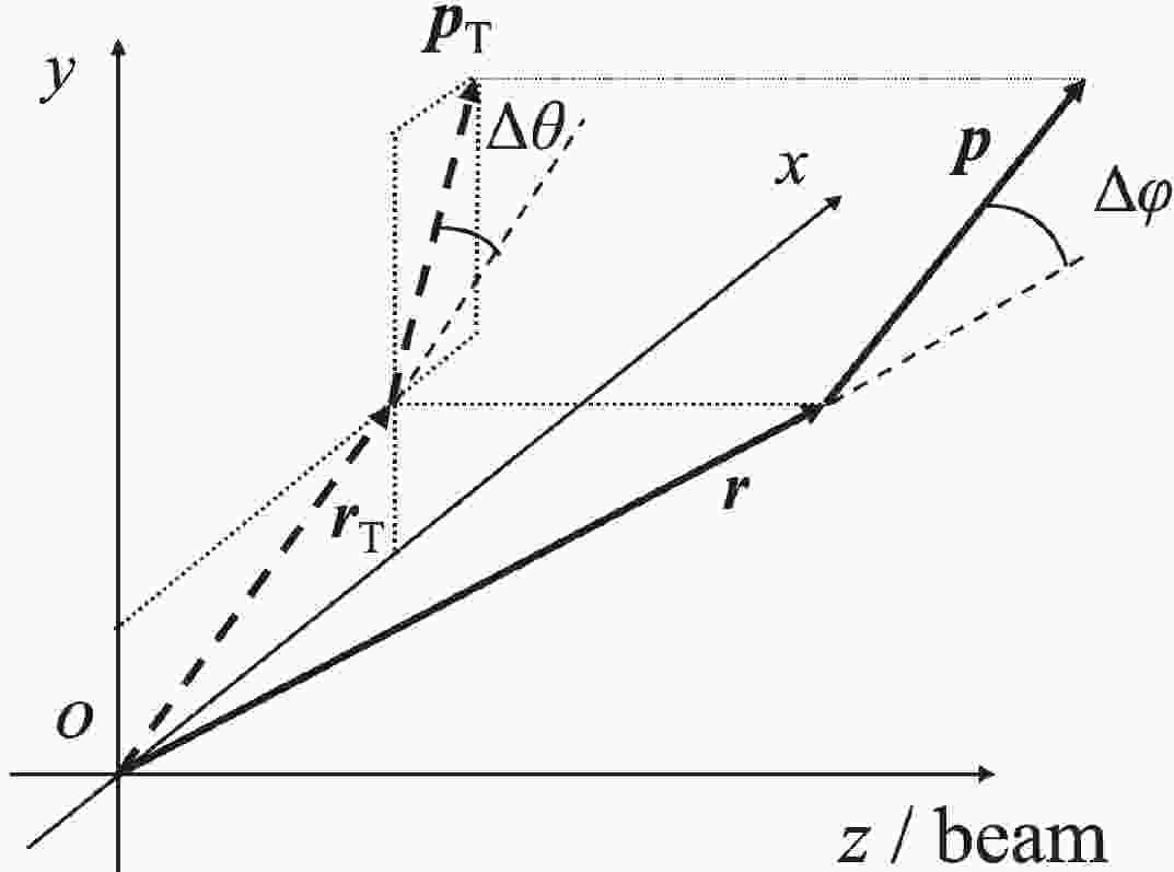
Many collaborations have already presented some HBT results for different collisions and energies [11-14]. When the HBT radii for the same collision energy were analyzed, the radii decreased with increasing transverse momentum of the pion pairs. This phenomenon, known as the transverse momentum dependence of HBT radii, is attributed to the space-momentum correlation [15, 16], which is caused by the collective flow [17]. We can obtain more information about the collective flow by studying the transverse momentum dependence of the HBT radii, making it important to study this space-momentum correlation. Hence, we introduce the single-particle space-momentum angle distribution to describe this space-momentum correlation. When the particles freeze out, there will be a finite angle between the radius vector and the momentum vector. Figure 1 displays the diagram of this angle and its projection angle $ \Delta \theta $ on the transverse plane. Here, the single-particle space-momentum angle distribution is the quantification of the space-momentum correlation [18]. As this paper focuses on the transverse plane, we only employ the angle $ \Delta \theta $.

Figure 1.  Diagram of $ \Delta\varphi $ and $ \Delta \theta $. $ \Delta\varphi $ is the angle between $ {{\boldsymbol{r}}} $ and $ {{\boldsymbol{p}}} $, and $ \Delta \theta $ is the angle between $ {\boldsymbol{r}}_{\rm{T}} $ and $ {\boldsymbol{p}}_{\rm{T}} $, at the freeze-out time. The origin is the center of the source.

In this study, a multiphase transport (AMPT) model is used to produce particles and calculate the HBT radius. The AMPT model is a hybrid model, which describes relativistic heavy ion collisions [19], and has already been widely used for HBT analysis [20-22]. We will also focus on how the single-particle space-momentum angle $ \Delta \theta $ distribution changes with the transverse momentum dependence on the transverse plane. The HBT radius $ R_{\rm{s}} $ is directly related to the transverse size of the pion source [23], so we attempt to deduce a numerical connection between the $ \Delta \theta $ distribution and the transverse momentum dependence of the HBT radius $ R_{\rm{s}} $.

This paper is structured as follows. Sec. II briefly introduces the AMPT model and the method used to calculate the HBT radii. In Sec. III, we calculate the HBT radii for pions at different collision energies. In Sec. IV, a numerical connection is constructed between the $ \Delta \theta $ angle distribution and the transverse momentum dependence of $ R_{\rm{s}} $. Finally, we summarize our conclusions in Sec. V.

The AMPT model is a hybrid model with initial particle distributions generated using the heavy ion jet interaction generator (HIJING) model. The AMPT model consists of two versions, the default AMPT model and the string melting AMPT model. The version employed here is the string melting AMPT model, which provides a good description of the two-pion correlation function [19, 24]. The string melting AMPT model consists of four main components: the initial conditions, partonic interactions, conversion from the partonic to hadronic matter, and hadronic interactions. It can provide better pion phase space information than our previous work, as well as a better $ \Delta \theta $ distribution.

The Correlation After Burner (CRAB) code is used to calculate the two-pion correlation functions [25]. The code is based on the formula

where $ {{\boldsymbol{q}}} = {{\boldsymbol{p}}}_1-{{\boldsymbol{p}}}_2 $, $ {{\boldsymbol{K}}} = ({{\boldsymbol{p}}}_1+{{\boldsymbol{p}}}_2)/2 $, $ \psi_{\rm{rel}} $ is the two particle wave function, and $ S(x,{{\boldsymbol{p}}}) $ is the emission function of the single particle, which describes the probability of emitting a particle with momentum $ {\boldsymbol{p}} $ at space-time point $ x $. In further discussion, we neglect the Coulomb interaction and strong interactions between pions and focus on the mid-rapidity range ($ -0.5<\eta<0.5 $).

The HBT three-dimensional correlation function can be written as [26]

where $ \lambda $ is the coherence parameter, and $ R_{\rm{o}} $, $ R_{\rm{s}} $, and $ R_{\rm{l}} $ are the HBT radii in the "out-side-long" coordinate system, where o, s, and l are the directions shown in Fig. 2. The longitudinal direction is along the beam direction, while the transverse plane is perpendicular to the longitudinal direction. In the transverse plane, the momentum direction of particle pairs is the outward direction. The direction perpendicular to the outward direction is referred to as the sideward direction. The HBT radii can be calculated using Eq. (2) to fit the HBT correlation function generated by the CRAB code.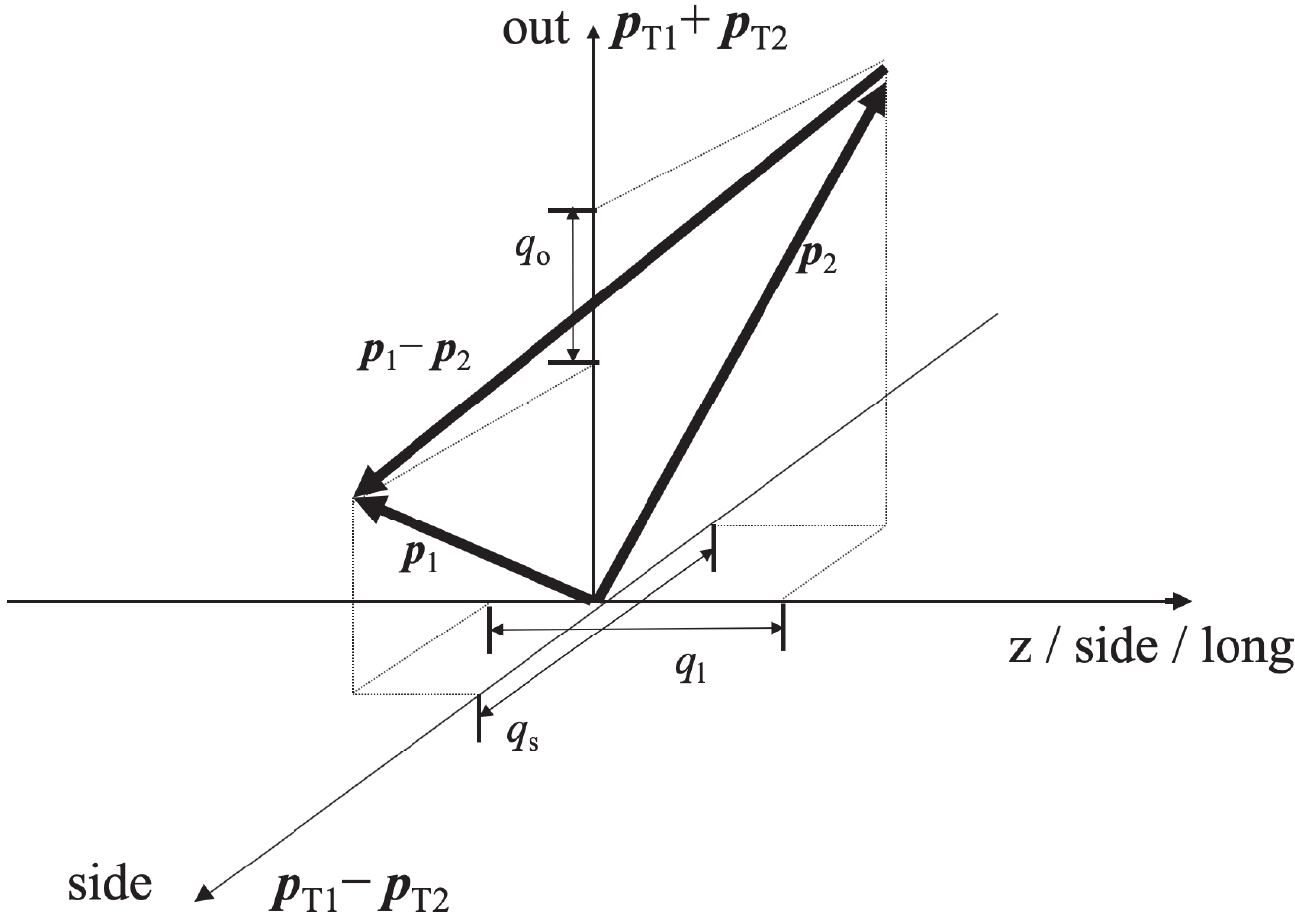

Figure 2.  Diagram of the "out-side-long" (o-s-l) coordinate system.

In HBT analysis, $ R_{\rm{s}} $ is directly related to the transverse size of the emission source, while $ R_{\rm{o}} $ and $ R_{\rm{l}} $ are influenced by the source lifetime and the velocity of the particles [16]. Therefore, $ R_{\rm{s}} $ is more important in this study, so we focus only on the transverse momentum dependence of $ R_{\rm{s}} $.

We employ the melting AMPT model to generate central Au+Au collision events at $ \sqrt{S_{NN}}$ = 19.6, 27, 39, 62.4, 200 GeV, with these energies chosen from the BES energies and the impact parameter as 0 fm. The Coulomb interaction and strong interactions are neglected, meaning the three types of pions can be treated as the same. The correlation function of the pions is calculated for different transverse momenta by the Crab code. An example of the correlation function of pions is shown in Fig. 3.

Figure 3.  (color online) Correlation function in the $ q_{\rm{o}} $ and $ q_{\rm{s}} $ directions of the central Au+Au collisions at $ \sqrt{S_{NN}} = 200 $ MeV for the AMPT model. The $ K_{\rm{T}} $ range is 175-225 MeV/c, and the $ q_{\rm{l}} $ range is 0-6 MeV/c.

Next, we employ Eq. (2) to fit the HBT correlation functions and obtain values of $ R_{\rm{s}} $ for different transverse momenta at different collision energies, as shown in Fig. 4.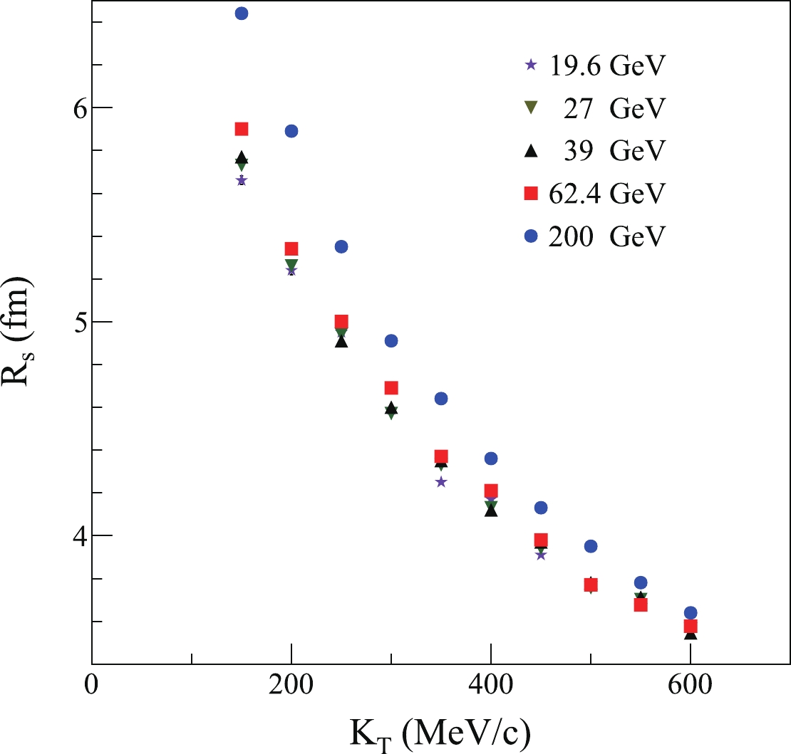

Figure 4.  (color online) Transverse momentum dependence of $ R_{\rm{s}} $ in AMPT model.

For all collision energies, $ R_{\rm{s}} $ decreases with increasing transverse momentum of the pairs, and they also demonstrate different strengths of $ K_{\rm{T}} $ dependence of $ R_{\rm{s}} $. The values of $ R_{\rm{s}} $ with higher $ K_{\rm{T}} $ are more similar. We can fit the HBT radii using

where parameter $ a $ is a common constant, and parameter $ b $ reflects how the HBT radii change with $ K_{\rm{T}} $; it describes the strength of the $ K_{\rm{T}} $ dependence of HBT radii. The collision energy dependence of parameter $ b $ is shown in Fig. 5.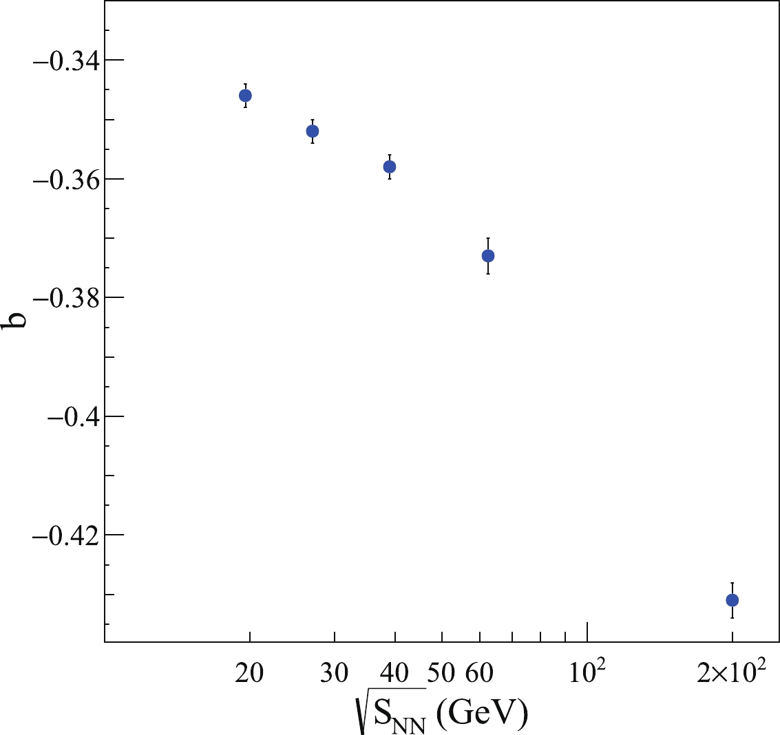

Figure 5.  (color online) Collision energy dependence of parameter $ b $ in the AMPT model.

In Fig. 5, with increasing collision energy, the values of parameter $ b $ for $ R_{\rm{s}} $ also increase (i.e., a larger $ |b| $), indicating a stronger $ K_{\rm{T}} $ dependence. In our previous study, we found that HBT radii can be influenced by the $ {\rm cos}(\Delta \theta) $ distribution, and the $ {\rm cos}(\Delta \theta) $ distribution changes with the pair momentum $ K_{\rm{T}} $, leading to changes in the HBT radius $ R_{\rm{s}} $ and the $ b $ value. Thus, we only focus on the dependence of the $ {\rm cos}(\Delta \theta) $ distribution on the parameter $ b $.

When the particles freeze-out, there is an angle between the radius vector and the momentum vector called the single-particle space-momentum angle, defined by $ \Delta \theta $ in the transverse momentum plane. We generally calculate the cosine value of this angle. There is substantial particle freeze-out from the source, so we calculate $ \cos(\Delta \theta) $ values for all particles to obtain the $ \cos(\Delta \theta) $ distribution. This distribution can directly detail the transverse momentum $ K_{\rm{T}} $ dependence of $ R_{\rm{s}} $ [18]. We use the pions, which are generated from the AMPT model and used to calculate the HBT correlation function, to obtain the $ \cos(\Delta \theta) $ distribution. Pions with random $ {\boldsymbol{p}}_{\rm{T}} $ and $ {\boldsymbol{r}}_{\rm{T}} $ are generated and used to calculate the random $ \cos(\Delta\theta) $ distribution. Then, we use the distribution of $ \cos(\Delta\theta) $ for different $ K_{\rm{T}} $ regions, which are calculated from the AMPT model and divided by the random $ \cos(\Delta\theta) $ distribution, to obtain the normalized $ \cos(\Delta\theta) $ distribution, as shown in Fig. 6.

Figure 6.  (color online) Normalized $ \cos(\Delta\theta) $ distribution for melting AMPT model.

In Fig. 6, with increasing transverse momentum $ K_{\rm{T}} $ and collision energies, the normalized $ \cos(\Delta \theta) $ distribution becomes closer to $ \cos(\Delta \theta) = 1 $. This phenomenon indicates that with the increase of transverse momentum $ K_{\rm{T}} $ and collision energy of the two pions, the momentum direction of a single-pion is closer to the space direction. Additionally, the transverse momentum dependence of HBT can be explained with the transverse momentum dependence of the normalized single-particle space-momentum angle $ \Delta \theta $ distribution. In our previous studies, we employed an exponential function to fit the normalized $ \Delta \theta $ distribution in a simple cylinder source. While the AMPT model is a hybrid model, the density of the source and the collective flow of the AMPT model is quite different from the cylinder source. Therefore, we modified our fit function to a double exponential to obtain better fitting results. Hence, the parameters set in this paper are different from our previous work. The fit functions of the fit lines are

where $ c_{1} $ and $ c_{2} $ are fit parameters, and the value 0.0005 was chosen by us to obtain good fitting results. The value of $ c_{1} $ is influenced by the proportion of the pions whose freeze-out direction is perpendicular to the radius direction, and $ c_{2} $ is influenced by the strength of the curve approach pion. They are both determined by the normalized $ \cos(\Delta \theta) $ distribution and are influenced by the collective flow. The velocity of the flow in different $ K_{\rm{T}} $ regions is shown in Fig. 7.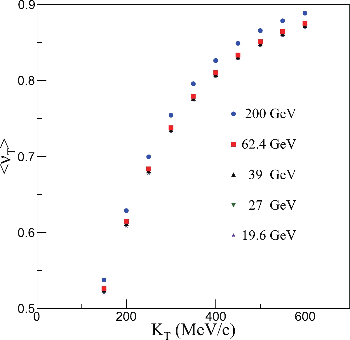

Figure 7.  (color online) Velocity of the flow for melting AMPT model.

In Fig. 7, the pions with higher transverse momentum are emitted by the larger collective flow, with the flow typically strong enough that the direction of freeze-out pions is limited to the flow direction, which means that $ \cos(\Delta \theta) $ approaches one. This results in the behavior of the normalized $ \cos(\Delta \theta) $ distribution in Fig. 6 and is reflected in the changing values of $ c_{1} $ and $ c_{2} $ with the collective flow. These values are shown in Fig. 8. The tendency is higher for larger $ K_{\rm{T}} $ and larger collision energy.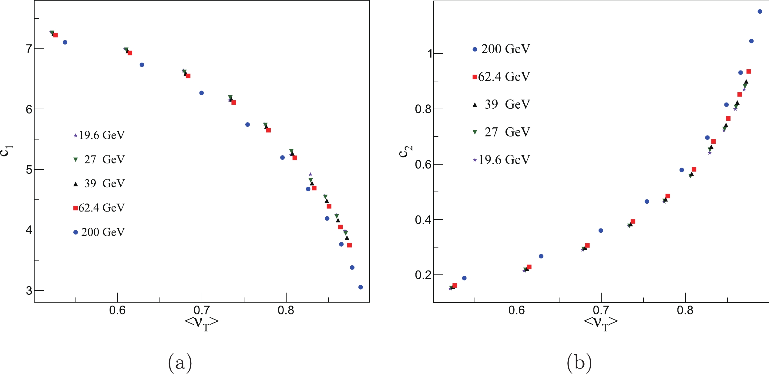

Figure 8.  (color online) Flow velocity dependence of fit parameters for $ c_{1} $ and $ c_{2}. $

Then, we discuss the normalized $ \cos(\Delta \theta) $ distribution changing with $ K_{\rm{T}} $. We use functions to describe how $ c_{1} $ and $ c_{2} $ change with $ K_{\rm{T}} $, seen as the fit lines in Fig. 9. These functions are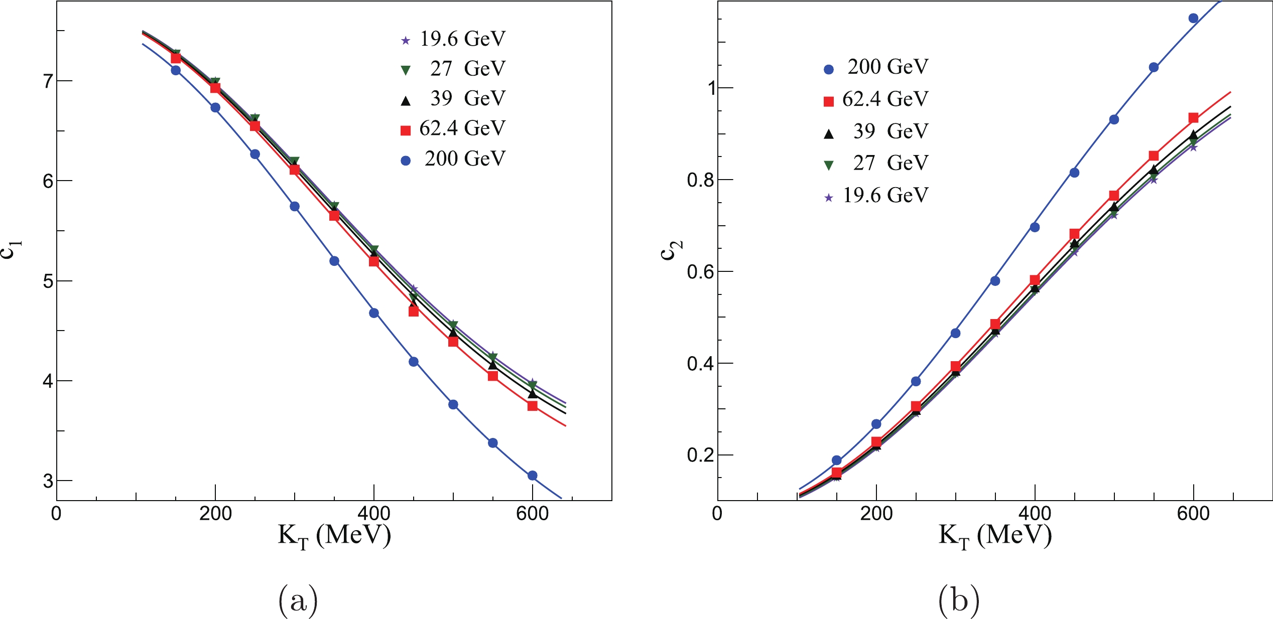

Figure 9.  (color online) Transverse momentum dependence of the fit parameters for $ c_{1} $ and $ c_{2}. $

where $ k $ and $ j $ are fit parameters; the values –4.5 and –3.5 were chosen by us to obtain a good fit. The parameters $ k_{1} $ and $ j_{1} $ are determined by the changes to $ c_{1} $ due to $ K_{\rm{T}} $. As $ K_{\rm{T}} \rightarrow +\infty $, the proportion of the pions with $ \cos(\Delta \theta) = 0 $ is at its lowest, affecting the $ j_{1} $ values. When $ K_{\rm{T}} = 0 $, this proportion is the highest, with the changing range of this proportion affecting the $ k_{1} $ values. The parameters $ k_{2} $ and $ j_{2} $ are determined by the changes to $ c_{2} $ with $ K_{\rm{T}} $, and when $ K_{\rm{T}} \rightarrow +\infty $, there is the greatest strength of the normalized $ \cos(\Delta \theta) $ distribution approaching one, affecting the $ j_{2} $ values. When $ K_{\rm{T}} = 0 $, this strength is the lowest, so the changing range of the strength affects the $ k_{2} $ values. In Fig. 9, at low collision energies, particularly for $ \sqrt{S_{NN}} $= 19.6, 27, and 39 GeV, the collision energies are very similar, as is the strength of collective flow. This results in the single-pion space-momentum angle having a similar distribution within the same transverse momentum region, meaning the $ c_{1} $ and $ c_{2} $ values are also similar.

In order to discuss how the normalized $ \cos(\Delta \theta) $ distribution changes with the strength of the $ K_{\rm{T}} $ dependence of $ R_{\rm{s}} $, we plot the parameter b, obtained from the transverse momentum dependence of $ R_{\rm{s}} $, as a function of the parameters $ k $ and $ j $, shown in Fig. 10. The changing pattern is carried by the fit parameters. The pattern indicates that parameter $ b $ has an extremum, so the effect of the single-pion space-momentum angle distribution on the HBT radii will be similar at higher energies, and the transverse momentum dependence of the HBT radii will also be similar at higher collision energies. This minimum value was set to –0.5, and the numerical relationship based on the fit results was then constructed. The red lines depict the fits, and the fit functions are

Figure 10.  (color online) Fit parameters in AMPT model. Parameter $ b $ is determined from the HBT radii fit function $ R = a p_{\rm{T}}^{b} $, and $ j_1 $, $ j_2 $ and $ k_1 $, $ k_2 $ are based on the fit function $ c_{1} = k_{1} \exp\Bigg[-4.5\times\Bigg(\dfrac{K_{\rm{T}}}{1000}\Bigg)^{2}\Bigg]+j_{1} $ and $ c_{2} = k_{2} \exp\Bigg[-3.5\times\Bigg(\dfrac{K_{\rm{T}}}{1000}\Bigg)^{2}\Bigg]+j_{2} $, where $ c_1 $ and $ c_2 $ are obtained from the normalized space-momentum angle distribution function $ f = 0.0005\exp\{ c_{1}\exp[c_{2}\cos(\Delta\theta)]\} $. The red lines are fits.

where $ \mu $ and $ \nu $ are fit parameters. These parameters are influenced by the change in the normalized $ \cos(\Delta \theta) $ distribution with the strength of the$ K_{\rm{T}} $ dependence of $ R_{\rm{s}} $. The fit parameter values are shown in Table 1.

	$c_1$		$c_2$
$\mu_{11}$	$60\pm20$	$\mu_{21}$	$0.219\pm0.005$
$\mu_{12}$	$-3.9\pm0.2$	$\mu_{22}$	$-3.0\pm0.2$
$\nu_{11}$	$0.023\pm0.002 $	$\nu_{21}$	$0.265\pm0.009 $
$\nu_{12}$	$1.7\pm0.1$	$\nu_{22}$	$-3.1\pm0.2$

Table 1.  Fit results of $ b(k) $ and $ b(j) $.

In short, the parameters $ c_{1} $ and $ c_{2} $ are determined by the normalized $ \cos(\Delta \theta) $ distribution. The proportion of pions whose $ \cos(\Delta \theta) = 0 $ determines the $ c_{1} $ values, and the strength of the normalized $ \cos(\Delta \theta) $ distribution approaching one determines the $ c_{2} $ values. The parameters $ k $ and $ j $ are determined by the distribution changing with pair momentum $ K_{\rm{T}} $, with $ k_{1} $ and $ j_{1} $ related to $ c_{1} $.$ k_{1} $ is influenced by the changing range of the proportion of pions with $ \cos(\Delta \theta) = 0 $, and $ j_{1} $ is influenced by the lowest proportion. $ k_{2} $ and $ j_{2} $ are also related to $ c_{2} $. $ k_{2} $ is influenced by the changing range of the strength of the normalized $ \cos(\Delta \theta) $ distribution approaching one, and $ j_{2} $ is influenced by its highest strength. Parameter $ b $ describes the strength of the transverse momentum dependence of $ R_{\rm{s}} $, and the parameters $ \mu $ and $ \nu $ describe how $ k $ and $ j $ change with $ b $, which is the connection between the single-pion space-momentum $ \cos(\Delta \theta) $ distribution and the transverse momentum dependence of the HBT radius $ R_{\rm{s}} $. With the AMPT model, a numerical connection has been established. When we obtain a series of $ R_{\rm{s}} $ data in different $ K_{\rm{T}} $ regions, we can estimate the $ \cos(\Delta \theta) $ distribution as a function of $ K_{\rm{T}} $. With further research, the values chosen can also be improved with more accurate fits.

The transverse momentum dependence of HBT radii is related to the space-momentum correlation, and the single-particle space-momentum angle $ \cos(\Delta \theta) $ distribution was used to quantify this correlation. Thus, the transverse momentum dependence of HBT radii can be explained by the transverse momentum dependence of the single-particle space-momentum angle $ \cos(\Delta \theta) $ distribution. With the string melting AMPT model, we calculated the transverse momentum of the HBT radius $ R_{\rm{s}} $ for several collision energies, with the results suggesting that, with increasing collision energies, the decrease in the HBT radii with the pair momentum is more prominent. Then, we calculated the single-particle space-momentum angle $ \cos(\Delta \theta) $ distribution for each pair momentum region and collision energy. The results indicate that, with increasing collision energies and pair momentum, the freeze-out directions of the pions are closer to the radius direction. We use several fit functions to establish a connection between these distributions and the $ R_{\rm{s}} $. With this connection, we can describe how the space-momentum correlation changes with increasing collision energies and also obtain information about the final stage of the Au+Au collision at the time the freeze-out occurs. Near the CEP, anomalies can occur in a wide variety of dynamic properties, which can affect the single-particle space-momentum correlation. It is also possible to see some non-monotonic behaviors through HBT analysis. With further research, HBT analysis may help us to learn more about the freeze-out stage of the collisions, and the critical effect of single-particle space-momentum correlations.