Generalized Crewther relation and a novel demonstration of the scheme independence of commensurate scale relations up to all orders

The Crewther relation [1, 2] provides a non-trivial relation for three fundamental constants, $ 3S = K R' $, where S is the anomalous constant of $ \pi^0\to\gamma\gamma $, K is the coefficient of the Bjorken sum rules for polarized deep-inelastic electron scattering [3], and $ R' $ is the isovector part of the cross-sectional ratio for electron-positron annihilation into hadrons [4]. In the theory of quantum chromodynamics (QCD) [5, 6], an improved Crewther relation is known as the “Generalized Crewther Relation (GCR)” [7-13]:

or

where $ a_s = \alpha_s/\pi $, $ D^{\rm{NS}} $ is the non-singlet Adler function, $ C^{\rm{Bjp}} $ is derived from the Bjorken sum rules for polarized deep-inelastic electron scattering, D is the Adler function, and $ C^{\rm{GLS}} $ is the coefficient of the Gross-Llewellyn Smith (GLS) sum rules [14]. The $ \Delta^{*}_{\rm{csb}} $ and $ \Delta_{\rm{csb}} $ are conformal breaking terms. For example, the $ \Delta_{\rm{csb}} $-term takes the form

where $ \beta(a_s) = -\sum_{i\geqslant 0}\beta_{i} a_s^{i+2} $ is the usual $ \beta $-function, and the coefficient $ K_k $ is free of $ \{\beta_i\} $-functions.

The perturbative QCD (pQCD) corrections to $ D^{\rm{NS}} $ and the Bjorken sum rules have been computed up to $ {\cal{O}}(\alpha_s^3) $-level [15-19] and $ {\cal{O}}(\alpha_s^4) $-level [20, 21], respectively. The GCR (1) between the non-singlet Adler function and the Bjorken sum rules was discussed in Refs. [22-24]. The GCR (2) between the Adler function and the GLS sum rules was investigated up to $ {\cal{O}}(\alpha_s^3) $-level in Ref. [10]. Using the known $ \alpha_s^4 $-order corrections [25, 26], we can derive a more accurate GCR (2) up to $ {\cal{O}}(\alpha_s^4) $-level. It is well-known that a physical observable is independent of any choice of theoretical conventions, such as the renormalization scheme and renormalization scale. This property is called “renormalization group invariance” (RGI) [27-31]. For a fixed-order pQCD prediction, if the perturbative coefficient preceeding $ \alpha_s $ and the corresponding $ \alpha_s $-value at each order are not consistent with each other, the RGI is explicitly broken [32, 33]. Conventionally, the “guessed” typical momentum flow of the process is adopted as the optimal renormalization scale with the purpose of eliminating the large logs to improve pQCD convergence, minimize the contributions from higher-order loop diagrams, or achieve a theoretical prediction in agreement with the experimental data. Such an approach directly breaks the RGI and reduces the predictive power of pQCD. Therefore, it is important to employ a proper scale-setting approach to achieve a scale-invariant fixed-order prediction.

In the literature, the principle of maximum conformality (PMC) [34-37] was proposed to eliminate the two artificial ambiguities. The purpose of PMC is not to find an optimal renormalization scale but to fix an effective $ \alpha_s $ for the process using the renormalization group equation (RGE). The PMC prediction satisfies all self-consistency conditions of the renormalization group [38]. Two multi-scale approaches have been suggested to achieve the goal of PMC, which are both equivalent in terms of perturbative theory [39], with a collection of their successful applications found in Ref. [40]. For the multi-scale approach, the PMC sets the scales in an order-by-order manner; the individual scales at each order reflect the varying virtuality of the amplitudes at those orders. It has been noted that the PMC multi-scale approach has two types of residual scale dependence due to unknown perturbative terms [41]. Those residual scale dependences suffer from both $ \alpha_s $-power suppression and exponential suppression, but their magnitudes may be large due to poor convergence of the perturbative series of either the PMC scale or the pQCD approximant [42].

Recently, the PMC single-scale approach [43] has been suggested to suppress the residual scale dependence by introducing an overall effective $ \alpha_s $. The argument for such an effective $ \alpha_s $ corresponds to the overall effective momentum flow of the process, which is also independent of any choice of renormalization scale. It has been shown that by using the PMC single-scale approach and the C-scheme strong coupling constant [44], one can achieve a strict demonstration of the scheme-invariant and scale-invariant PMC prediction up to any fixed order [45]. Moreover, the resulting renormalization scheme- and scale-independent conformal series is useful not only for achieving precise pQCD predictions but also for producing reliable predictions of the contributions of unknown higher-orders. Some of these applications have been investigated in Refs. [46-50], which are estimated by using the Padé resummation approach [51-53]. In this study, we adopt the PMC single-scale approach to deal with the GCR (2), and then, for the first time, we estimate the unknown $ 5_{\rm{th}} $-loop contributions for GCR (2). A novel demonstration of the scheme independence of the commensurate scale relation for all orders is also presented.

It is helpful to define the effective charge for a physical observable [54-56], which incorporates the entire radiative correction into its definition. For example, the GLS sum rules indicate that the isospin singlet structure function $ xF_3(x,Q^2) $ satisfies an unsubtracted dispersion relation [14], i.e.,

where $ xF_3(x,Q^2) = xF^{\nu p}_3(x,Q^2)+xF^{\bar{\nu} p}_3(x,Q^2) $, and Q is the momentum transfer. All of the radiative QCD corrections can be defined as an effective charge $ a_{F_3}(Q) $. Moreover, the Adler function of the cross-sectional ratio for electron-positron annihilation into hadrons [4] can be written as

where

The Adler function D can be defined as the effective charge $ a_D(Q) $. Thus, the Adler function D and the GLS sum rules coefficient $ C^{\rm{GLS}} $ can be rewritten as

The effective charges $ a_D(Q) $ and $ a_{F_3}(Q) $ are by definition pQCD calculable, which can be expressed in the following perturbative form:

where $ {\cal{S}} = D $ or $ {F_3} $, respectively, $ r^{\cal{S}}_{i,j = 0} $ are conformal coefficients with $ r^{\cal{S}}_{1,0} = 1 $, and $ r^{\cal{S}}_{i,j\neq0} $ are nonconformal coefficients. The $ \beta $-pattern for each order is determined by RGE [35, 37]. The coefficients $ r^{D, F_3}_{i,j} $ up to the four-loop level under the $ \overline{\rm{MS}} $ scheme can be determined from Refs. [21, 57] using the general QCD degeneracy relations [39].

After applying the PMC single-scale approach [43], all $ \{\beta_i\} $-terms are used to fix the correct $ \alpha_s $-value by using the RGE, up to four-loop accuracy, and we obtain the following conformal series:

where $ {\tilde Q}_* $ and $ {\hat Q}_* $ are in perturbative series, which can be derived from the pQCD series of $ a_D $ and $ a_{F_3} $. $ {\tilde Q}_* $ and $ {\hat Q}_* $ correspond to the overall momentum flows of the effective charges $ a_D(Q) $ and $ a_{F_3}(Q) $, which are independent of any choice of renormalization scale. This property confirms that the PMC is not for choosing an optimal renormalization scale but for determining the correct momentum flow of the process. Using the four-loop pQCD series of $ a_D $ and $ a_{F_3} $, we determine their magnitudes up to N²LL accuracy by replacing the coefficients $ {\hat r}_{i,j} $ in Eqs. (8)-(11) of Ref. [43] with $ r^D_{i,j} $ or $ r^{F_3}_{i,j} $, respectively. We present $ {\tilde Q}_* $ and $ {\hat Q}_* $ for different accuracies in Fig. 1. As shown in Fig. 1, as the perturbative series of $ a_D $ and $ a_{F_3} $ exhibit good perturbative convergence, it is interesting to find that their magnitudes up to different accuracies, such as the leading log (LL), next-to-leading log (NLL), and next-next-leading log (N²LL), are very similar. Thus, one can treat the N²LL-accurate $ {\tilde Q}_* $ and $ {\hat Q}_* $ as their exact values.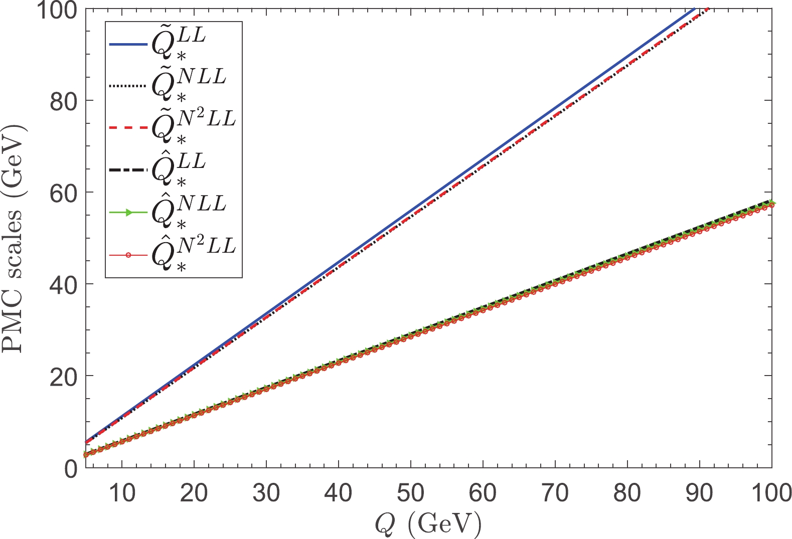

Figure 1.  (color online) PMC scales ${\tilde Q}_*$ and ${\hat Q}_*$ versus the momentum scale Q up to LL, NLL, and N²LL accuracies.

By applying the PMC single-scale approach, one can improve the precision of $ D(a_s) $ and $ C^{\rm{Bjp}}(a_s) $. Fig. 2 shows the PMC predictions of $ D(a_s) C^{\rm{GLS}}(a_s) $ up to two-loop, three-loop, and four-loop levels. Moreover, the PMC scheme-invariant and scale-invariant conformal series provides a reliable platform for predicting the uncalculated high-order terms [46]. For the first time, we also present the previously uncalculated five-loop result in Fig. 2, which is predicted using the Padé approximation approach (PAA) [51-53] and the preferable [N/M] = [0/n-1]-type Padé generating function, which makes the PAA geometric series self-consistent with the PMC prediction [46]. More explicitly, the PAA has been introduced for estimating the $ (n+1)_{\rm{th}} $-order coefficient for a given $ n_{\rm{th}} $-order perturbative series and for feasible conjectures on the likely high-order behavior of the series. For example, with the following conformal series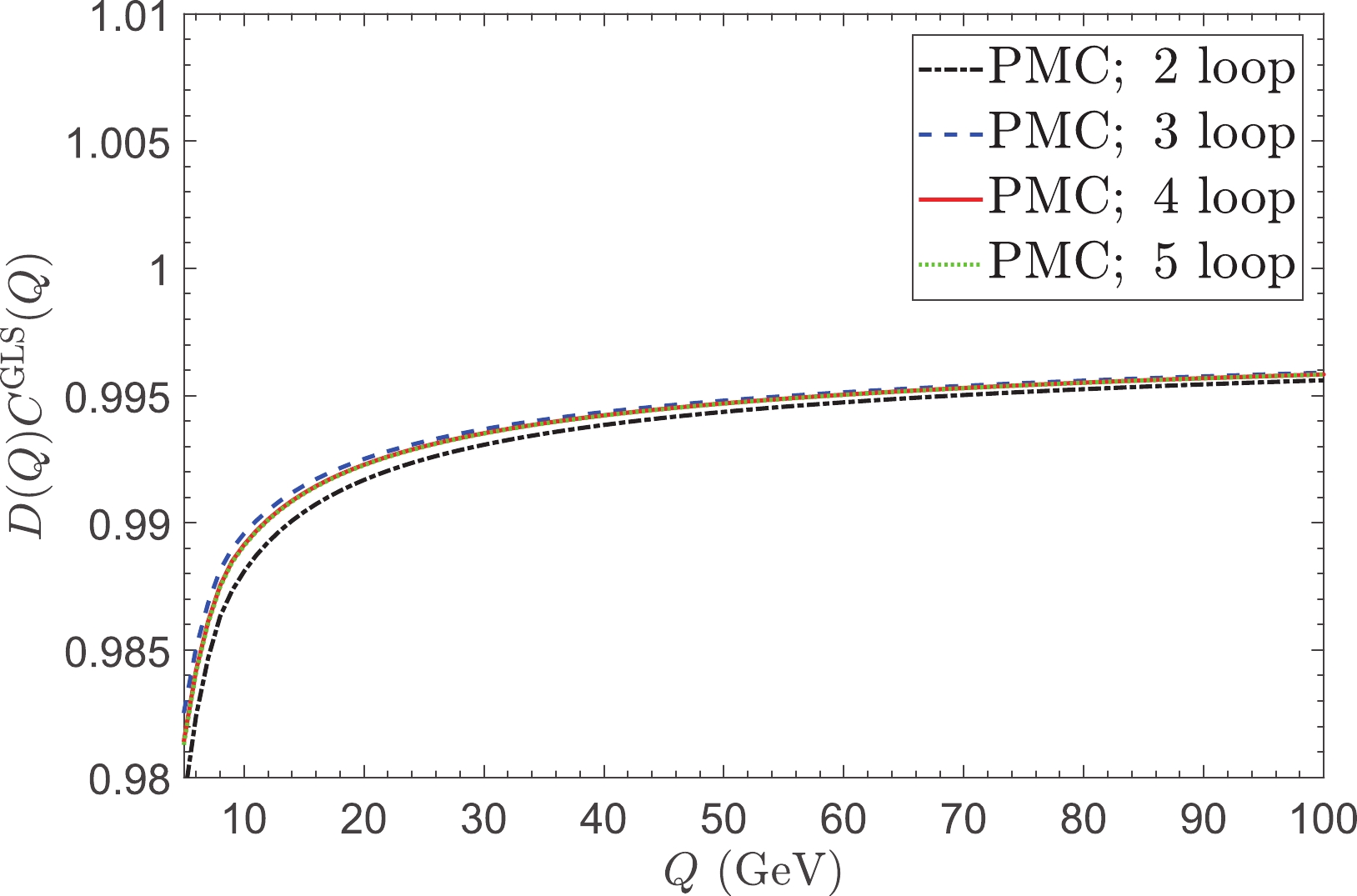

Figure 2.  (color online) $D(a_s) C^{\rm{GLS}}(a_s)$ versus momentum Q under the PMC single-scale approach up to the two-loop, three-loop, and four-loop levels. The uncalculated five-loop result is predicted using the Padé approximation approach.

for the present cases, we have $ n = 4 $ and $ \rho(Q) = a_D|_{\rm{PMC}} $ or $ a_{F_3}|_{\rm{PMC}} $. Its $ [N/M] $-type fractional generating function from the PAA is defined as

where $ M\geqslant 1 $ and $ N+M = n-1 $. Then the unknown $ (n+1)_{\rm{th}} $-order coefficient $ r_{n+1,0} $ can be predicted using the known coefficients $ \{r_{1,0},\cdots,r_{n,0}\} $ by expanding the fractional generating function over $ a_s $. That is, Eq. (13) can be expressed as

We can first express all coefficients $ \{b_0,\cdots,b_N\} $ and $ \{c_1,\cdots,c_M\} $ by the known coefficients $ r_{\{1,\cdots,n\},0} $ and then obtain the coefficient $ r_{n+1,0} $ over $ \{b_i\} $ and $ \{c_i\} $, which can be finally expressed by $ \{r_{1,0},\cdots,r_{n,0}\} $. The PAA predictions of $ a_D|_{\rm{PMC}} $ and $ a_{F_3}|_{\rm{PMC}} $ are presented in Table 1 and Table 2, respectively, in which the known coefficients (“Exact”) for different orders are also presented for comparison. This suggests that with more known perturbative terms, the PAA predicted coefficients are closer to the “Exact” values.

	${\rm{Exact}}$	${\rm{PAA}}$
$r^D_{1,0}$	1	−
$r^D_{2,0}$	1.84028	−
$r^D_{3,0}$	−3.03222	[0/1]: 3.38662
$r^D_{4,0}$	−23.2763	[0/2]:−17.3926
$r^D_{5,0}$	−	[0/3]:−34.1991

Table 1.  The preferable [0/n-1]-type PAA predictions of three-, four-, and five-loop coefficients of $a_{D}|_{\rm{PMC}}$ for the PMC single-scale approach. The known coefficients (“Exact”) are also presented as comparisons.

	${\rm{Exact}}$	${\rm{PAA}}$
$r^{F_3}_{1,0}$	1	−
$r^{F_3}_{2,0}$	0.840278	−
$r^{F_3}_{3,0}$	−5.71277	[0/1]: 0.706067
$r^{F_3}_{4,0}$	−16.0776	[0/2]:−10.1939
$r^{F_3}_{5,0}$	−	[0/3]: 18.2157

Table 2.  The preferable [0/n-1]-type PAA predictions of three-, four-, and five-loop coefficients of $a_{F_3}|_{\rm{PMC}}$ for the PMC single-scale approach. The known coefficients (“Exact”) are also presented as comparisons.

Figure 2 shows that the two-, three-, four-, and five-loop predictions have similar curves, particularly the predicted five- and four-loop curves. This is because the PMC conformal series is free of renormalon divergence [58-60], which inversely results in good pQCD convergence. The scheme-independent $ D(a_s)|_{\rm{PMC}} $ and $ 1/C^{\rm{GLS}}(a_s)|_{\rm{PMC}} $ have the same conformal coefficients, but as shown in Fig. 1, their PMC scales are not identical, $ {\tilde Q}_*\neq{\hat Q}_* $. Thus, there is a small deviation from unity:

This deviation, though it is very small in the large Q region, e.g., for $ Q\simeq10^3 $ GeV, where the ratio is approximately $ 0.998 $ for the five-loop prediction, is part of the intrinsic nature of QCD theory due to its conformal breaking property.

In GCR (2), the scheme dependent $ \Delta_{\rm{csb}} $-term has been introduced to collect all the conformal breaking terms. This leads to explicit scheme dependence of GCR (2) under the conventional scale-setting approach due to the mismatching of $ \alpha_s $ and its corresponding expansion coefficients. Conversely, by applying the PMC single-scale approach, we can achieve an exact scheme and scale invariant GCR at any fixed order. More explicitly, after applying the PMC single-scale approach, we obtain the following conformal series,

where all the coefficients are exactly equal to $ 1 $, and the PMC scale $ Q_* $ is independent of the choice of renormalization scale, which can be fixed up to N²LL accuracy using the known four-loop coefficients, i.e.,

where

The scale $ Q_* $ satisfies Eqs. (8)-(11) of Ref. [43], whose value can be determined by replacing $ a_s $ and $ {\hat r}_{i,j} $ with $ a_{F_3} $ and $ r^{D F_3}_{i,j} $. The $ r^{D F_3}_{i,j} $ is a function of $ r^D_{i,j} $ and $ r^{F_3}_{i,j} $ [37]. One can derive Eqs.(18)-(20) by substituting those functions into Eqs. (9)-(11) of Ref. [43]. Eq. (16) is exactly scheme-independent and can be treated as a kind of commensurate scale relation (CSR). The CSR has been suggested in Ref. [61] for the purpose of ensuring the scheme-independence of the pQCD approximants among different renormalization schemes, with all original CSRs suggested in Ref. [61] at the NLO level. The PMC single-scale approach provides a method of extending the CSR to any order. A general demonstration of the scheme independence of the CSR (16) is presented in the next section. As a special case, taking the conformal limit that all $ \{\beta_i\} $-terms tend to zero, we have $ Q_* \to Q $, and the relation (16) becomes the original Crewther relation [9]:

By applying the PMC single-scale approach, one can obtain similar scheme-independent relations among different observables. The relation (16) not only provides a fundamental scheme-independent relation but also has phenomenologically useful consequences.

For example, the effective charge $ a_{F_3} $ can be related to the effective change $ a_R $ of the R-ratio for the $ e^+e^- $ annihilation cross section ($ R_{e^+e^-} $). The measurable R-ratio can be expressed by the perturbatively calculated Adler function, i.e.,

where $ q_f $ is the electric charge of the active flavor. Similarly, the perturbative series of the effective charge $ a_R(Q) $ can be written as

where the coefficients $ r^R_{i,j} $ under the $ \overline{\rm{MS}} $-scheme can be derived from Refs. [20, 21, 26, 57]. Here, we will not consider the nonperturbative contributions, which may be important in small $ Q^2 $-region [62-71], but are negligible for comparatively large s and $ Q^2 $. After applying the PMC single-scale approach, we obtain a relation between $ a_R $ and $ a_{F_3} $ up to N³LO, i.e.,

with the first four coefficients

where $ \gamma^{{\rm{S}}, {\rm{NS}}}_{i} $ are singlet and non-singlet anomalous dimensions which are unrelated to $ \alpha_s $-renormalization, and the effective PMC scale $ \bar{Q}_* $ can be determined up to N²LL accuracy, which reads

where

and

Experimentally, the effective charge $ a_R $ has been constrained by measuring $ R_{e^+e^-} $ above the thresholds for the production of the $ (c\bar{c}) $-bound state [72], i.e.

Substituting it into Eq. (24), we obtain

which is consistent with the PMC prediction derived directly from Eq. (11) within errors, e.g.,

where the first error is for $ \Delta Q = \left(^{+1.48}_{-1.26}\right)\; {\rm{ GeV}} $ and the second error is for $ \Delta\alpha_{s}(M_Z) = 0.1179\pm0.0011 $ [73]. At present, the GLS sum rules are measured at small $ Q^2 $-values [74, 75], and an extrapolation of the data gives [76]

which agrees with our prediction within errors.

In this section, we present a novel demonstration of the scheme independence of CSR for all orders by relating different pQCD approximants within the effective charge method. The effective charge $ a_A $ can be expressed as a perturbative series over another effective charge $ a_B $,

where $ a_A $ and $ a_B $ are the effective charges under arbitrary schemes A and B, respectively. The previously mentioned $ a_D $ and $ a_{F_3} $ are examples of effective charges. The $ \{\beta_i\} $-functions are usually calculated under the $ \overline{\rm{MS}} $-scheme, and the $ \{\beta_i\} $-functions for $ A/B $ scheme can be obtained using its relation to the $ \overline{\rm{MS}} $-scheme, i.e. $ \beta^{A/B} = {\partial \alpha_{s, A/B}}/{\partial \alpha_{s, \overline{\rm{MS}}}}{\beta^{\overline{\rm{MS}}}} $. The effective charge $ a_B $ at any scale $ \mu $ can be expanded in terms of a C-scheme coupling $ \hat{a}_B(\mu) $ at the same scale [45], i.e.,

where by choosing a suitable C, the coupling $ {\hat a}_{B} $ can be equivalent to $ a_B $ defined for any scheme at the same scale, i.e., $ a_B = {\hat a}_{B}|_{C} $. By using the C-scheme coupling, the relation (37) becomes

where the coefficients $ r_i $ are

Following the standard PMC single-scale approach, we obtain the following CSR:

where the effective PMC scale $ Q_{**} $ is obtained by vanishing all nonconformal terms, which can be expanded as a power series over $ {\hat a}_{B}(Q_{**}) $, i.e.,

whose first three coefficients are

and

One may observe that only the LL coefficient $ \hat{S}_{0} $ depends on the scheme parameter C, and all higher order coefficients $ \hat{S}_{i} $ ($ i\geqslant 1 $) are independent of C.

Moreover, the C-scheme coupling $ {\hat a}_{B}(Q_*) $ satisfies the following relation [45],

Substituting Eq. (45) into the right hand side of this equation, we obtain

By employing this equation, we can derive a solution for $ {\hat a}_{B}(Q_{**}) $. As all the coefficients in Eq. (50) are independent of C at any fixed order, the magnitude of $ {\hat a}_{B}(Q_{**}) $ shall be exactly free of C. Together with the scheme-independent conformal coefficients and the fact that the value of C can be chosen to match any renormalization scheme, we can conclude that the CSR (44) is exactly scheme independent. This example can be extended to all orders.

The PMC provides a systematic approach to determine an effective $ \alpha_s $ for a fixed-order pQCD approximant. By using the PMC single-scale approach, the determined effective $ \alpha_s $ is scale-invariant, which is independent of any choice of renormalization scale. As all nonconformal terms have been eliminated, the resultant pQCD series is scheme independent, satisfying the requirements of RGI. Furthermore, by applying the PMC single-scale approach, we obtain a scheme-independent GCR, $ D(a_s)|_{\rm{PMC}}C^{\rm{GLS}}(a_s)|_{\rm{PMC}} \approx 1 $, which provides a significant connection between the Adler function and the GLS sum rules. We have shown that their corresponding effective couplings satisfy a scheme-independent CSR, $ a_D(Q) = $$ \displaystyle\sum_{i = 1}^{n} a_{F_3}^i(Q_*) $. Furthermore, we obtain a CSR that relates the effective charge $ a_{F_3} $ to the effective charge of R-ratio, $ a_{F_3}(Q) = \displaystyle\sum_{i = 1}^{4} r_{i,0} a^{i}_R(\bar{Q}_*) $. This leads to $a_{F_3}(Q = $ $ 12.58^{+1.48}_{-1.26}\; {\rm{GeV}}) = 0.073^{+0.025}_{-0.026}$, which agrees with the extrapolated measured value within errors. A demonstration on the scheme-independence of the CSR has been presented. The scheme- and scale- independent CSRs shall provide important tests of pQCD theory.