Processing math: 66%

Measurements of natCd(γ, x) reaction cross sections and isomer ratio of 115m,gCd with the bremsstrahlung end-point energies of 50 and 60 MeV

  • The flux-weighted average cross sections of natCd(γ, xn)115g,m,111m,109,107,105,104Cd and natCd(γ, x)113g,112,111g,110mAg reactions were measured at the bremsstrahlung end-point energies of 50 and 60 MeV. The activation and off-line γ-ray spectrometric technique was carried out using the 100 MeV electron linear accelerator at the Pohang Accelerator Laboratory, Korea. The natCd(γ, xn) reaction cross sections as a function of photon energy were theoretically calculated using the TALYS-1.95 and the EMPIRE-3.2 Malta codes. Then, the flux-weighted average cross sections were obtained from the theoretical values of mono-energetic photons. These values were compared with the flux-weighted values from the present study and were found to be in general agreement. The measured experimental reaction cross-sections and integral yields were described for cadmium and silver isotopes in the natCd(γ, xn)115g,m,111m,109,107,105,104Cd and natCd(γ, x)113g,112,111g,110mAg reactions. The isomeric yield ratio (IR) of 115g,mCd in the natCd(γ, xn) reaction was determined for the two bremsstrahlung end-point energies. The measured isomeric yield ratios of 115g,mCd in the natCd(γ, xn) reaction were also compared with the theoretical values of the nuclear model codes and previously published literature data of the 116Cd(γ, n) and 116Cd(n, 2n) reactions. It was found that the IR value increases with increasing projectile energy, which demonstrates the characteristic of excitation energy. However, the higher IR value of 115g,mCd in the 116Cd(n, 2n) reaction compared to that in the 116Cd(γ, n) reaction indicates the role of compound nuclear spin alongside excitation energy.
  • The Schwinger pair production of charged particles is an important QED phenomenon that is related to the vacuum instability and persistence in the presence of strong external electromagnetic fields [1]. Another important spontaneous pair production phenomenon is the Hawking radiation from black holes, which can be viewed as a tunneling process through the black hole horizon [2]. A charged black hole thus provides a natural lab in which both the Schwinger pair production and the Hawking radiation can occur and mix with each other. Usually the equation of motions (EoMs) of quantum fields in a general black hole background is difficult to solve analytically in full spacetime. However, when the symmetry of the spacetime geometry is enhanced under some conditions, the problem becomes manageable; for this reason, in a series of recent studies, the spontaneous pair production of charged particles has been systematically studied in near extremal charged black holes, including the RN black hole [3-5] and the Kerr-Newman (KN) black hole [6, 7], in which the near horizon geometry is enhanced into AdS2 or warped AdS3 in the near extremal limit. Owing to the enhanced near horizon symmetry, the explicit forms of the pair production rate and other 2-point correlation functions have been obtained and their holographic descriptions have been found based on the RN/CFT [8-13] and KN/CFTs dualities [14-16]. In addition to charged black hole backgrounds, pair production has also been investigated in pure AdS or dS spacetime, see, e.g., [17-20], whereas in the absence of a gravitational field, the pure Schwinger effect has been efficiently analyzed by using the phase-integral method [21-24].

    However, previous studies mainly focused on analyzing spontaneous pair production in the near horizon region of black holes in an asymptotically flat spacetime. A charged black hole in AdS spacetime has an additional AdS symmetry at the asymptotical boundary. From the holographic point of view, the CFT description of pair production has been revealed only in the near horizon region in terms of AdS2/CFT1 (or warped AdS3/CFT2). Although particle pairs produced in the near horizon region of black holes indeed provide important contributions to those in full spacetime, an understanding of the whole picture is still lacking. In the present paper, we extend the study of pair production to a full near extremal RN-AdS5 black hole background, which possesses an AdS5 geometry at the asymptotic spatial boundary as well as an AdS2 structure in the near horizon region. It is shown that the radial equation of the charged scalar field propagating in this spacetime can be transformed into a Heun-like differential equation and thus be solved by matching its solutions in the near and far spacetime regions, using the low temperature limit. Consequently, analytical forms of the full solutions for the pair production rate, the absorption cross section ratio, and the retarded Green's functions are obtained, and they are shown to have concise relations with their counterparts calculated in the near horizon region. Based on these concise relations, numerical analysis can easily be performed, and the pair production rate in full spacetime is shown to be smaller than that in the near horizon region, which is consistent with the assumption that pair production mainly comes from the black hole near horizon region.

    A near extremal RN-AdS5 black hole is also a very useful background for studying holographic dualities. As the near horizon AdS2 (or warped AdS3) spacetime is dual to a 1D CFT (or chiral CFT2), while asymptotical AdS5 spacetime is dual to another 4D CFT, the former is called IR CFT, while the latter is called UV CFT, and they are connected with each other via the holographic renormalization group (RG) flow along the radial direction [25-27]. For example, it has been shown that a near extremal RN-AdS black hole acts as a holographic model in describing typical properties of a (non)Fermi liquid at the quantum critical point [28-31]. It is thus natural and interesting to find holographic descriptions of pair production in an RN-AdS5 black hole both in the IR CFT1 in the near horizon region and the UV CFT4 at the asymptotical AdS5 boundary. We show that the picture in the IR CFT1 is very similar to those in the near extremal RN and KN black holes, and that the pair production rate and the absorption cross section ratio calculated from the AdS2 spacetime can be matched with those from the dual IR CFT. Regarding the UV 4D CFT, a direct comparison of calculations between the bulk and the boundary in terms of the AdS5/CFT4 is not made due to a lack of information on the dual finite temperature CFT4 side. However, from the bulk gravity side, the condition for pair production in the full near extremal RN-AdS5 spacetime is the violation of the Breitenlohner-Freedman (BF) bound [32, 33] in AdS5 spacetime. This, on the dual 4D CFT side, corresponds to a complex conformal weight for the scalar operator dual to the bulk charged scalar field, which indeed indicates instabilities for the scalar operator on the boundary and is consistent with the situation in the IR CFT. Furthermore, we determined an interesting relation between the full pair production rate and the absorption cross section ratio via changing the roles of sources and operators simultaneously both in the IR and the UV CFTs.

    The rest of the paper is organized as follows. In Sec. II, we provide a brief review of the bulk theory and consider the near horizon geometry of an RN- AdSd+1 black hole and the EoMs of the probe charged scalar field. In Sec. III, spontaneous pair production in the near horizon region of near extremal RN- AdSd+1 black holes is discussed, and the 2-point functions of the charged scalar field (such as the retarded Green's function), pair production rate, and absorption cross section ratio are calculated. In Sec. IV, the full analytical solution for the radial equation of the charged scalar field in RN-AdS5 black holes is obtained by applying the matching technique. Consequently, the full analytical forms of the pair production rate, absorption cross section ratio, and retarded Green's function are found, and the connections with their counterparts in the near horizon region of the black hole are discussed. Then, in Sec. V, the dual CFTs descriptions of spontaneous pair production are both analyzed in terms of the AdS2/CFT1 correspondence in the IR region and the AdS5/CFT4 correspondence in the UV region, and their connections are also revealed. Finally, the conclusion and physical implications are provided in Sec. VI.

    The d+1 dimensional Einstein-Maxwell theory has an action (in units of c==1) as

    I=dd+1xg[116πGd+1(R+d(d1)L2)1g2sFμνFμν],

    (1)

    where L is the curvature radius of the asymptotical AdSd+1 spacetime, and gs is the dimensionless coupling constant of the U(1) gauge field. The dynamical equations

    Rμν12gμνRd(d1)2L2gμν=8πGd+1g2s(4FμλFνλgμνFαβFαβ),μ(gFμν)=0,

    (2)

    admit the Reissner-Nordström-Anti de Sitter (RN-AdSd+1) black brane (or the planar black hole) solution [34]

    ds2=L2r2f(r)dr2+r2L2(f(r)dt2+dx2i),A=μ(1rd2ord2)dt,

    (3)

    with

    f(r)=1Gd+1L2Mrd+Gd+1L2Q2r2d2,μ=d12(d2)gsQrd2o,

    (4)

    where ro is the radius of the outer horizon (f(ro)=0), μ is the chemical potential with dimension [μ]=length(d1)/2, M is the mass, and Q is the charge of the black brane. We may find an explicit expression of ro for d=4 from a solution of the cubic equation, which is complicated, but ro has a general expression in the extremal case, i.e., r in IIB. The condition f(ro)=0 gives M=rdoGd+1L2+Q2rd2o (which is the Smarr-like relation related to the first law of thermodynamics of the black brane); temperature T and “surface” entropy density s of the black brane are, respectively,

    T=rod4πL2(1d2dGd+1L2Q2r2d2o),s=14Gd+1(roL)d1.

    (5)

    Moreover, the first law of thermodynamics of the dual boundary d-dimensional quantum field is

    δϵ=Tδs+μδρc,

    (6)

    where the “surface” energy and charge densities are, respectively,

    ϵ=d116πLd1M,ρc=2(d1)(d2)8πgsLd1Q.

    (7)

    Then, it is straightforward to check the Euler relation

    (dd1)ϵ=ϵ+p=Ts+μρc,

    (8)

    where the pressure is p=ϵd1, which shows that the dual d-dimensional quantum field theory on the asymptotic boundary is conformal, as expected.

    To make the following analysis convenient, let us introduce the length scale r2d2d2dGd+1L2Q2; then, the temperature can be rewritten as

    T=rod4πL2(1r2d2r2d2o).

    (9)

    Note that r may be treated as the “effective” radius of the inner black hole horizon though f(r)0 in general and r<ro. The extremal condition for a degenerate horizon at ro=r is M=M02(d1)d2rdGd+1L2. The near extremal limit of the near horizon is obtained by taking the limit ε0 of the transformations

    MM0=d(d1)rd2Gd+1L2ε2ρ2o,ror=ερo,rro=ε(ρρ0),t=τε,

    (10)

    where in general ρo is finite and ρ[ρ0,).

    Expanding f(r) around r=ro, we have

    f(r)d(d1)r2o(ρ2ρ2o)ε2+O(ε3),

    (11)

    the near horizon geometry is given by

    ds2=ρ2ρ2o2dτ2+2dρ2ρ2ρ2o+r2oL2dx2i,A=(d2)μro(ρρo)dτ,

    (12)

    where 2L2d(d1) is defined as the square of the curvature radius of the effective AdS2 geometry. The limit ρo0 yields the extremal limit.

    The solution in Eq. (12) can also be written in the Poincaré coordinates in terms of ξ=2/ρ, (|ξ|ξo=2/ρo),

    ds2=2ξ2((1ξ2ξ2o)dτ2+dξ21ξ2ξ2o)+r2oL2dx2i,A=(d2)μ2ro(1ξ1ξo)dτ.

    (13)

    The above geometry is a black brane with both local and asymptotical topology AdS2×Rd1 (AdS2 has the SL(2,R)R symmetry). The horizons of the new black brane are located at ξ=±ξo, and its temperature is Tn=12πξo. Note that if we adopt the new coordinates zξ/ξo with |z|1 and η=τ/ξo, the metric becomes

    ds2=2z2((1z2)dη2+dz21z2)+r2oL2dx2i,

    (14)

    and the temperature associated with the inverse period of η is normalized to ˜Tn=12π.

    The action of a bulk probe charged scalar field Φ with mass m and charge q is

    S=dd+1xg(12DαΦDαΦ12m2ΦΦ),

    (15)

    where DααiqAα with α being the covariant derivative in curved spacetime. The corresponding Klein-Gordon (KG) equation is

    (αiqAα)(αiqAα)Φ=m2Φ.

    (16)

    Moreover, the radial flux of the probe field is

    F=iggrr(ΦDrΦΦDrΦ).

    (17)

    In the RN-AdSd+1 background (3), assuming Φ(t,x,r)=ϕ(r)eiωt+ikx, the KG Eq. (16) has the radial form

    (Lr)d1r(rd+1Ld+1f(r)r)ϕ(r)+(L2(ω+qAt)2r2f(r)m2L2r2k2)ϕ(r)=0.

    (18)

    The solutions to Eq. (18) cannot be directly found in terms of special functions in the full spacetime region. In what follows, we solve it in different regions and match these solutions to obtain the full solution.

    Firstly, we analyze the near horizon, near extreme region (13) and solve the KG Eq. (16) by expanding the scalar field as

    Φ(τ,x,ξ)=ϕ(ξ)eiwτ+ikx.

    (19)

    Then, the KG equation reduces to

    ξ2(1ξ2ξ2o)ϕ(ξ)2ξ3ξ2oϕ(ξ)+ξ2(w+qAτ)21ξ2ξ2oϕ(ξ)=m2eff2ϕ(ξ),

    (20)

    where the effective mass square is defined as m2eff=m2+L2k2r2o, or the KG equation can be expressed in the z coordinate as

    z2(1z2)ϕ(z)2z3ϕ(z)+z21z2[(wξo+qeff1zz)2m2eff21z2z2]ϕ(z)=0,

    (21)

    where the effective charge of the probe field is qeff(d2)μroq. The singularities of Eq. (21) are located at z=0,z=±1 and z=.

    To find the solutions, we determine the indices at each singular point. For z0, setting ϕ(z)zˉα, the leading terms in Eq. (21) are

    z2ϕ(z)+(q2effm2eff)2ϕ(z)=0,

    (22)

    which gives

    ˉα=12±121+4(m2effq2eff)212±121+4˜m2eff212±ν.

    (23)

    For z1, setting ϕ(z)(1+z)ˉβ, Eq. (21) reduces to

    2(1+z)ϕ(z)+2ϕ(z)+(wξo2qeff)22(1+z)ϕ(z)=0,

    (24)

    and the index is

    ˉβ=±i(wξo2qeff)=±i(w4πTnqeff).

    (25)

    Finally, for z1, setting ϕ(z)(1z)ˉγ, Eq. (21) reduces to

    2(1z)ϕ(z)2ϕ(z)+(wξo)22(1z)ϕ(z)=0,

    (26)

    from which

    ˉγ=±iwξo2=±iw4πTn=±iω/ε4π/(2πξo)=±iω2ερo/2=±iω4πT

    (27)

    is obtained. Further, imposing the ingoing boundary condition at the black brane horizon z=1 requires ˉγ=iwξo2=iw4πTn.

    Also, note that Eq. (21) can be rewritten in a more explicit form as

    ϕ(z)+(1z+1+1z1)ϕ(z)+(˜m2eff2z+12(wξo2qeff)2z+1+12w2ξ2oz1)ϕ(z)z(z+1)(z1)=0,

    (28)

    which becomes the Fuchs equation with three canonical singularities a1, a2 and a3, as follows:

    ϕ(z)+(1ˉα1ˉα2za1+1ˉβ1ˉβ2za2+1ˉγ1ˉγ2za3)ϕ(z)+(ˉα1ˉα2(a1a2)(a1a3)za1+ˉβ1ˉβ2(a2a3)(a2a1)za2+ˉγ1ˉγ2(a3a1)(a3a2)za3)ϕ(z)(za1)(za2)(za3)=0,

    (29)

    where a1=0, a2=1, and a3=1 and

    ˉα1=12±ν,ˉα2=12ν,ˉβ1=ˉβ2=±iwξo2qeff2,ˉγ1=ˉγ2=±iwξo2,

    (30)

    and ˉα1+ˉα2+ˉβ1+ˉβ2+ˉγ1+ˉγ2=1 is satisfied. The Fuchs Eq. (29) can be transformed into the standard hypergeometric function

    ζ(1ζ)ψ(ζ)+[˜γ(1+˜α+˜β)ζ]ψ(ζ)˜α˜βψ(ζ)=0,

    (31)

    via the conformal coordinate transformation

    ζ=(a2a3)(za1)(a2a1)(za3),ϕ(z)=(za1za3)ˉα1(za2za3)ˉβ1ψ(ζ),

    (32)

    where ˜α=ˉα1+ˉβ1+ˉγ1,˜β=ˉα1+ˉβ1+ˉγ2 and ˜γ=1+ˉα1ˉα2. (Note that one can freely choose the indices i=1,2 for ˉαi, ˉβi and ˉγi.)

    For Eq. (28), we have ζ=2z/(z1),˜α=12±ν+iwξoiqeff,˜β=12±νiqeff,˜γ=1±2ν. Therefore, the explicit solutions in the near horizon near extreme region are

    ϕ(z)=c1(zz1)12+ν(z+1z1)iwξo2iqeff2F1(12+ν+iwξoiqeff,12+νiqeff;1+2ν;2zz1)+c2(zz1)12ν(z+1z1)iwξo2iqeff2F1(12ν+iwξoiqeff,12νiqeff;12ν;2zz1).

    (33)

    At the horizon of the AdS2 black brane, z=1, Eq. (33) is expanded as follows:

    ϕ(z)=c(in)H(1z)iw4πTn+c(out)H(1z)iw4πTn,

    (34)

    where

    c(in)H=c1()12νiw2πTn+iqeff212ν+iw4πTnΓ(1+2ν)Γ(iw2πTn)Γ(12+ν+iqeff)Γ(12+ν+iw2πTniqeff)

    +c2()12+νiw2πTn+iqeff212+ν+iw4πTnΓ(12ν)Γ(iw2πTn)Γ(12ν+iqeff)Γ(12ν+iw2πTniqeff),

    (35)

    and

    c(out)H=c1()12νiw2πTn+iqeff212νiw4πTnΓ(1+2ν)Γ(iw2πTn)Γ(12+νiqeff)Γ(12+νiw2πTn+iqeff)+c2()12+νiw2πTn+iqeff212+νiw4πTnΓ(12ν)Γ(iw2πTn)Γ(12νiqeff)Γ(12νiw2πTn+iqeff).

    (36)

    In contrast, at the AdS2 boundary, z0, the asymptotic expansion of Eq. (33) is

    ϕ(z)=c2()12ν+iw4πTniqeffz12ν+c1()12+ν+iw4πTniqeffz12+ν=A(w,k)z12ν+B(w,k)z12+ν,

    (37)

    where A is the source of the charged scalar field in the bulk AdS2, while B is the response or the operator ˆO(w,k) (in the momentum space) of the boundary CFT1 (i.e., the IR CFT) dual to the charged scalar field in the bulk AdS2 background. Note that in order to obtain the propagating modes, ν should be purely imaginary, which can be set as νi|ν|, i.e., ϕ(z)=c(out)Bz12i|ν|+c(in)Bz12+i|ν|. It was shown in [3] that the condition of an imaginary ν is equivalent to the violation of the BF bound in AdS2 spacetime, namely

    ˜m2eff<142,

    (38)

    which corresponds to a complex conformal weight of the scalar operator in the dual IR CFT.

    1   Pair production rate and absorption cross section ratio

    The Schwinger pair production rate |b|2 and the absorption cross section ratio σabs can be calculated from the radial flux by imposing different boundary conditions

    F=i(roL)d1(1z2)(ΦzΦΦzΦ),

    (39)

    which gives

    F(in)B=2|ν|(roL)d1|c(in)B|2,F(out)B=2|ν|(roL)d1|c(out)B|2,F(in)H=w2πTn(roL)d1|c(in)H|2,F(out)H=w2πTn(roL)d1|c(out)H|2,

    (40)

    where F(in)B and F(out)B are the ingoing and outgoing fluxes at the AdS2 boundary, while F(in)H and F(out)H are the ingoing and outgoing fluxes at the AdS2 black brane horizon, respectively.

    The Schwinger pair production rate |bAdS2|2 can be computed either by choosing the inner boundary condition or the outer boundary condition, which gives the same result [3], e.g., by adopting the outer boundary condition, i.e., F(in)B=0, (c(in)B=0c1=0),

    |bAdS2|2=F(out)BF(in)H=4πTn|ν|w|c(out)Bc(in)H|2=8πTn|ν|w|Γ(12i|ν|+iqeff)Γ(12i|ν|+iw2πTniqeff)Γ(12i|ν|)Γ(iw2πTn)|2=2sinh(2π|ν|)sinh(w2Tn)coshπ(|ν|qeff)coshπ(|ν|w2πTn+qeff).

    (41)

    Similarly, by adopting the outer boundary condition, the absorption cross section ratio is computed as

    σAdS2abs=F(out)BF(out)H=4πTn|ν|w|c(out)Bc(out)H|2=8πTn|ν|w|Γ(12i|ν|iqeff)Γ(12i|ν|iw2πTn+iqeff)Γ(12i|ν|)Γ(iw2πTn)|2=2sinh(2π|ν|)sinh(w2Tn)coshπ(|ν|+qeff)coshπ(|ν|+w2πTnqeff).

    (42)

    The pair production rate and the absorption cross section ratio are connected by the simple relation

    |bAdS2|2=σabs(|ν||ν|).

    (43)

    It was shown that the abovementioned relation also holds for a charged scalar field [11] and for a charged spinor field [4], both in a four-dimensional near extremal RN black hole.

    2   Retarded Green's function

    The two-point retarded Green's function of the boundary operator dual to the bulk charged scalar field is computed through

    GAdS2R(w,k)ˆOˆOR=2F|z0B(w,k)A(w,k)+contactterms

    (44)

    by taking the inner boundary condition, i.e., F(out)H=0, which gives

    c2c1=()12ν22νΓ(1+2ν)Γ(12νiqeff)Γ(12νiw2πTn+iqeff)Γ(12ν)Γ(12+νiqeff)Γ(12+νiw2πTn+iqeff).

    (45)

    Thus, the two-point retarded Green's function is

    GAdS2R(w,k)B(ω,k)A(ω,k)=()2νc1c2=()4ν122νΓ(12ν)Γ(12+νiqeff)Γ(12+νiw2πTn+iqeff)Γ(1+2ν)Γ(12νiqeff)Γ(12νiw2πTn+iqeff).

    (46)

    In addition, the corresponding boundary condition (F(in)B=0 and F(out)H=0) is used to obtain the quasinormal modes of the charged scalar field in AdS2 spacetime, which correspond to the poles of the retarded Green's function of dual operators (with complex conformal weight hR=12+ν) in the IR CFT, namely

    12+νiw2πTn+iqeff=Nw=2πTn(qeffiNihR),N=0,1,.

    (47)

    Eq. (47) gives the quasinormal modes of the charged scalar field perturbation.

    In this section, we describe our study of the pair production for the whole spacetime of RN-AdS5. Like before, we need to solve the corresponding radial Klein equation for the scalar field.

    To find the solution in the full region, we focus on d=4 and the near extremal cases. By introducing the coordinate transformation ϱ=r2M (and denoting M = Gd+1L2M, ϱo=r2oM and ϱ=r2M), the radial Eq. (18) can be expressed as

    ϕ(ϱ)+(1ϱϱ1+1ϱϱ2+1ϱϱo)ϕ(ϱ)+(ϱ(˜ωϱ˜qμϱo)2(ϱϱ1)2(ϱϱ2)2(ϱϱo)2˜m2ϱ+˜k2(ϱϱ1)(ϱϱ2)(ϱϱo))ϕ(ϱ)=0,

    (48)

    where the parameters are ˜ω=L2(ω+qμ)2M, ˜q=L2q2M, ˜m=Lm2, ˜k=L2|k|2M and

    ϱ1=12ϱo12ϱo2+8ϱ3ϱo,ϱ2=12ϱo + 12ϱo2+8ϱ3ϱo.

    (49)

    Further, defining another coordinate

    yϱϱoϱo,aϱ2ϱoϱo,bϱ1ϱoϱo,

    (50)

    the metric of the RN-AdS5 black hole becomes

    ds2=L2dy24(1+y)2f(y)+r2oL2(1+y)(f(y)dt2+dx2i),A=μy1+ydt,

    (51)

    where

    f(y)=1Mr4o(1+y)2+Q2r6o(1+y)3,Q2=Gd+1L2Q2.

    (52)

    Moreover, Eq. (48) transforms into

    ϕ(y)+(1y+1ya+1yb)ϕ(y)+((˜ω(y+1)˜qμ)2(y+1)y2(ya)2(yb)2˜m2(y+1)ϱo+˜k2y(ya)(yb))ϕ(y)ϱo=0.

    (53)

    To solve ϕ(y), first, we determine its exponents at the corresponding singularities 0, a, b, and , which are α1,2, β1,2, γ1,2, and δ1,2, respectively,

    α1,2=±i(˜ω˜qμ)abϱo=±iω4πT,β1,2=±i(˜ω(1+b)˜qμ)1+b(ab)bϱo,γ1,2=±i(˜ω(1+a)˜qμ)1+a(ba)aϱo,

    (54)

    where the index “1” corresponds to the “+” sign, and the index “2” corresponds to the “” sign. Then, decomposing ϕ(y) as

    ϕ(y)=(yyb)α1(yayb)γ1R(y),

    (55)

    we obtain

    R(y)+(1y+1ya+1yb2bα1y(yb)+2(ab)γ1(ya)(yb))R(y)+V2R(y)=0,

    (56)

    where

    V2(2+3aa2y)˜ω24(a+1)˜ω˜qμ+(a+2)˜q2μ2ϱoa2y(ya)(yb)2M1,

    (57)

    and

    M1=(ba)γ1y(ya)(yb)+2b(ab)α1γ1y(ya)(yb)2+˜m2(y+1)ϱo+˜k2ϱoy(ya)(yb)+bα1y(ya)(yb).

    (58)

    We divide the regions into a near region

    y=ϱϱoϱo1,

    (59)

    and a far region

    y=ϱϱoϱoa,

    (60)

    and an overlapping region, in which

    a1.

    (61)

    The physical reasoning of a1 relies on the observation that the temperature of a black hole is

    T=roπL2(1ϱ3ϱo3),

    (62)

    which gives a0 for T0, as

    a=321298πL2Tro.

    (63)

    We want to point out that the matching condition in Eq. (61) indicates that the near extremal condition is essential for matching the solutions in the near and far regions. It is not necessary for the frequency to be infinitely small; however, the frequency should definitely not be very large compared with the temperature T; otherwise, the backreaction to the background geometry cannot be ignored.

    Now we find the approximate solutions in different regions. First, by using the near region condition (y1), Eq. (53) reduces to

    ϕ(y)+(1y+1ya)ϕ(y)+((aα1iqeffy)2y2(ya)2+˜m2ϱo+˜k2ϱoby(ya))ϕ(y)=0.

    (64)

    Obviously Eq. (64) can be solved by the hypergeometric function as

    ϕ(y)=(ya)α1iqeff(c3yα12F1(α,β;γ;ya)+c4yα12F1(1γ+α,1γ+β;2γ;ya)),

    (65)

    where α=12+ν+2α1iqeff, β=12ν+2α1iqeff, and γ=1+2α1, and =L/12 is the radius of the effective AdS2 geometry in the near horizon region of the RN-AdS5 black hole. Second, in the far region, by using the condition (ya), Eq. (56) can turn into

    R(y)+(2y+1yb4bα1y(yb)+2ibqeffy(yb))R(y)+V3R(y)=0,

    (66)

    where

    V3˜ω2ϱoy(yb)2+4b2α1(α1iqeff)y2(yb)2b(2α1iqeff)y2(yb)˜m2(y+1)ϱo+˜k2ϱoy2(yb),

    (67)

    (where the relation γ1α1+i˜qμbϱo=α1iqeff when |a|1 is used). Similarly, Eq. (66) has a solution in terms of the hypergeometric function as

    ϕ(y)=(yb1)λ(c5yν122F1(α,β;γ;yb)+c6yν122F1(1γ+α,1γ+β;2γ;yb))

    (68)

    in which α=12+ν+Δ+λ, β=12+νΔ+λ, γ=1+2ν, Δ=1+˜m2, and λ=(iqeff)2˜ω2ϱob.

    In the overlapping region, one has the inequalities

    ay1<b

    (69)

    (1<b since b=32 + 1298πL2Tro3, as T0), which means |ay|0 and |yb|0, which transforms Eqs. (65) and (68) into the following forms: the near regionsolution

    ϕ(y)=((1)αc3Γ(γ)Γ(βα)Γ(β)Γ(γα)+(1)1+γαc4Γ(2γ)Γ(βα)Γ(1γ+β)Γ(1α))y12ν+((1)βc3Γ(γ)Γ(αβ)Γ(α)Γ(γβ)+(1)1+γβc4Γ(2γ)Γ(αβ)Γ(1γ+α)Γ(1β))y12+ν

    (70)

    and the far region solution

    ϕ(y)(1)λc5y12+ν+(1)λc6y12ν.

    (71)

    Comparing these two identities, one finds the connection relations

    c5=(1)λ((1)βc3Γ(γ)Γ(αβ)Γ(α)Γ(γβ)+(1)1+γβc4Γ(2γ)Γ(αβ)Γ(1γ+α)Γ(1β)),

    (72)

    c6=(1)λ((1)αc3Γ(γ)Γ(βα)Γ(β)Γ(γα)+(1)1+γαc4Γ(2γ)Γ(βα)Γ(1γ+β)Γ(1α)).

    (73)
    1   Pair production and absorption cross section

    Now we denote the radial flux of the charged scalar field in metric (51) as D:

    D=2ir4o(1+y)3f(y)L5(ϕ(y)yϕ(y)ϕ(y)yϕ(y)).

    (74)

    In the near horizon limit, i.e.,y0, Eq. (65) reduces to

    ϕ(y)=c3yα1(ya)α1iqeff+c4yα1(ya)α1iqeff,

    (75)

    where the first part is the outgoing mode, and the second part is the ingoing mode. Further, the asymptotic form of \phi(y) at the boundary ( y\to \infty ) of the AdS5 spacetime results in the form

    \phi(y) = A(\tilde{\omega}, \tilde{k})y^{- 1 + \Delta}+B(\tilde{\omega}, \tilde{k})y^{- 1 - \Delta},

    (76)

    where A(\tilde{\omega}, \tilde{k}) is the source of the charged scalar field in the bulk RN-AdS5 black hole, while B(\tilde{\omega}, \tilde{k}) is the response (the operator) of the boundary CFT4 (i.e., the UV CFT) dual to the charged scalar field in the bulk. As in the case of the AdS2 spacetime, the condition for the propagating modes requires an imaginary \Delta , i.e., \Delta = {\rm i}\left| \Delta \right| , which means

    m^2\leqslant -\frac{4}{L^2},

    (77)

    namely, the violation of the BF bound in AdS5 spacetime.

    Therefore, the corresponding outgoing and ingoing fluxes at the horizon and the boundary of the near extremal RN-AdS5 black brane are

    \begin{aligned}[b] {\cal D}_H^{(\mathrm{out})} & = \frac{{4\pi \omega T{r_{\mathrm{o}}}^2}}{{abL}}|{c_3}{|^2} = \frac{2r_{\mathrm{o}}^3\omega}{L^3}|c_3|^2 ,\\{\kern 1pt} {\cal D}_H^{(\mathrm{in})} &= - \frac{{4\pi \omega T{r_{\rm{o}}}^2}}{{abL}}|{c_4}{|^2} = -\frac{2r_{\mathrm{o}}^3\omega}{L^3}|c_4|^2, \\ {\cal D}_B^{({\mathrm{out}})} & = \frac{{4|\Delta |{r_{\rm{o}}}^4}}{{{L^5}}}\left| A( {\tilde \omega ,\tilde k})\right|^2,\\ {\cal D}_B^{({\mathrm{in}})}& = - \frac{{4|\Delta |{r_{\rm{o}}}^4}}{{{L^5}}}\left|B( {\tilde \omega ,\tilde k})\right|^2. \end{aligned}

    (78)

    The absorption cross section ratio \sigma _{\mathrm{abs}}^{\mathrm{AdS_5}} and the Schwinger pair production rate \left|\mathfrak{b}^{\mathrm{AdS_5}}\right|^2 can be calculated by choosing the inner boundary condition {\cal D}_H^{(\mathrm{out})} = 0 and ( c_3 = 0 ) and are given by

    \sigma _{{\rm{abs}}}^{{\rm{Ad}}{{\rm{S}}_{\rm{5}}}} = \left| {\frac{{{\cal D}_H^{({\rm{in}})}}}{{{\cal D}_B^{({\rm{in}})}}}} \right| = \frac{{{\rm{2}}T{L^{\rm{2}}}\left| \nu \right|\sinh \left( {2\pi \left| \Delta \right|} \right)}}{{{r_{\rm{o}}}{{\left| {H\left( {\nu ;\Delta ;\lambda } \right){{\left( {G_R^{{\rm{Ad}}{{\rm{S}}_{\rm{2}}}}} \right)}^{ - 1}} + H\left( { - \nu ;\Delta ;\lambda } \right)} \right|}^2}}}{\sigma _{{\rm{abs}}}},

    (79)

    and

    {\left| {{\mathfrak{b}^{{\text{Ad}}{{\text{S}}_{\text{5}}}}}} \right|^2} \!\!=\!\! \left| {\frac{{{\cal D}_H^{({\text{in}})}}}{{{\cal D}_B^{({\text{out}})}}}} \right| \!\!=\!\! \frac{{{\text{2}}T{L^{\text{2}}}\left| \nu \right|\sinh \left( {2\pi \left| \Delta \right|} \right)}}{{{r_{\rm{o}}}{{\left| {H\left( {\! -\! \nu ; \!-\! \Delta ;\lambda } \right)G_R^{{\text{Ad}}{{\text{S}}_{\text{2}}}} \!+\! H\left( {\nu ;\! -\! \Delta ;\lambda } \right)} \right|}^2}}}{\left| {{\mathfrak{b}^{{\text{Ad}}{{\text{S}}_{\text{2}}}}}} \right|^2},

    (80)

    where H\left( {x;y;z} \right) denotes a function

    H\left( {x;y;z} \right) \equiv {\left( { - 1} \right)^{2x}}{2^x}\frac{{\Gamma \left( {1 + {\rm{2}}x} \right)}}{{\Gamma \left( {\dfrac{1}{2} + x - y + z} \right)\Gamma \left( {\dfrac{1}{2} + x - y - z} \right)}},

    (81)

    and

    G_R^{\rm{AdS_2}} = {\left( { - 1} \right)^{4\nu - 1}}{2^{2\nu }}\frac{{\Gamma \left( {1 - 2\nu } \right)}}{{\Gamma \left( {1 + 2\nu } \right)}}\frac{{\Gamma \left( {\dfrac{1}{2} + \nu - {\rm i}{q_{{\rm{eff}}}}\ell } \right)}}{{\Gamma \left( {\dfrac{1}{2} - \nu - {\rm i}{q_{{\rm{eff}}}}\ell } \right)}}\frac{{\Gamma \left( {\dfrac{1}{2} + \nu - {\rm i}\dfrac{\omega }{{2\pi T}} + {\rm i}{q_{{\rm{eff}}}}\ell } \right)}}{{\Gamma \left( {\dfrac{1}{2} - \nu - {\rm i}\dfrac{\omega }{{2\pi T}}{\rm{ + }}{\rm i}{q_{{\rm{eff}}}}\ell } \right)}},

    (82)

    which is exactly the retarded Green's function in Eq. (46) of the IR CFT in the near horizon, near extremal region. Furthermore, {\sigma _{\mathrm{abs}}} and {\left| {{\mathfrak{b}^{{\text{Ad}}{{\text{S}}_{\text{2}}}}}} \right|^2} are exactly the absorption cross section ratio and the mean number of produced pairs of the corresponding IR CFT obtained from Eqs. (42) and (41). We find a relationship

    \left|\mathfrak{b}^{\mathrm{AdS_5}}\right|^2 = -\sigma _{\mathrm{abs}}^{\mathrm{AdS_5}}\left(\left| \nu \right| \to - \left| \nu \right|, \left| \Delta \right| \to - \left| \Delta \right|\right),

    (83)

    which is similar to Eq. (43) except for a combined change in signs in both |\nu| and |\Delta| .

    With Eq. (80) at hand we can easily investigate the relationship between the pair production rate in the near horizon and that for the whole spacetime of RN-AdS5. As shown in Fig. 1, we can see that the mean number of produced pairs for the whole spacetime is less than that from near horizon region. Moreover, with increasing charge of the scalar field, the corresponding ratio becomes smaller, which is consistent with previous assumptions stating that the Schwinger effect mainly occurs in the near horizon region.

    Figure 1

    Figure 1.  (color online) Ratio of mean number of produced pairs for the whole spacetime to that in the near horizon region as a function of \omega {L^2}/{r_{\rm{o}}} for different values of {q_{{\rm{eff}}}}\ell with T{L^{\text{2}}}/{{r_{\text{o}}}} = 0.001 , \nu = 0.1{\rm i} , and \Delta = 0.1{\rm i} (left); T{L^{\text{2}}}/{{r_{\text{o}}}} = 0.001 , \nu = 0.01{\rm i} , and \Delta = 0.01{\rm i} (middle); T{L^{\text{2}}}/{{r_{\text{o}}}} = 0.01 , \nu = 0.1{\rm i} , and \Delta = 0.1i (right).
    2   Retarded Green's function

    To calculate the retarded Green's function, an ingoing boundary condition is required, namely c_3 = 0 . Then, from Eqs. (72) and (73), the connection relations are

    {c_5} = {\left( { - 1} \right)^{ - 1 + \gamma - \beta - \lambda}}{c_4}\frac{{\Gamma \left( {2 - \gamma } \right)\Gamma \left( {\alpha - \beta } \right)}}{{\Gamma \left( {1 - \gamma + \alpha } \right)\Gamma \left( {1 - \beta } \right)}},

    (84)

    {c_6} = {\left( { - 1} \right)^{ - 1 + \gamma - \alpha - \lambda}}{c_4}\frac{{\Gamma \left( {2 - \gamma } \right)\Gamma \left( {\beta - \alpha } \right)}}{{\Gamma \left( {1 - \gamma + \beta } \right)\Gamma \left( {1 - \alpha } \right)}}.

    (85)

    Substituting Eqs. (84) and (85) into Eq. (68) and taking y \to \infty , namely the boundary of the AdS5 spacetime, one obtains

    \begin{aligned}[b] A(\tilde \omega ,\tilde k) = & \left( - 1 \right)^{{\rm i} q_{\rm{eff}}\ell - 2\lambda - 1 + \Delta }c_4\bigg( \frac{{\Gamma \left( {2 - \gamma } \right)\Gamma \left( {\alpha - \beta } \right)}}{{\Gamma \left( {1 - \gamma + \alpha } \right)\Gamma \left( {1 - \beta } \right)}}\frac{{\Gamma \left( {\gamma '} \right)\Gamma \left( {\alpha ' - \beta '} \right)}}{{\Gamma \left( {\alpha '} \right)\Gamma \left( {\gamma ' - \beta '} \right)}}+ \frac{{\Gamma \left( {2 - \gamma } \right)\Gamma \left( {\beta - \alpha } \right)}}{{\Gamma \left( {1 - \gamma + \beta } \right)\Gamma \left( {1 - \alpha } \right)}}\frac{{\Gamma \left( {2 - \gamma '} \right)\Gamma \left( {\alpha ' - \beta '} \right)}}{{\Gamma \left( {1 - \gamma ' + \alpha '} \right)\Gamma \left( {1 - \beta '} \right)}} \bigg),\\ \\ B(\tilde{\omega}, \tilde{k}) = & \left( - 1 \right)^{{\rm i} q_{\rm{eff}}\ell - 2\lambda - 1 - \Delta }c_4\bigg( \frac{{\Gamma \left( {2 - \gamma } \right)\Gamma \left( {\alpha - \beta } \right)}}{{\Gamma \left( {1 - \gamma + \alpha } \right)\Gamma \left( {1 - \beta } \right)}}\frac{{\Gamma \left( {\gamma '} \right)\Gamma \left( {\beta ' - \alpha '} \right)}}{{\Gamma \left( {\beta '} \right)\Gamma \left( {\gamma ' - \alpha '} \right)}}+ \frac{{\Gamma \left( {2 - \gamma } \right)\Gamma \left( {\beta - \alpha } \right)}}{{\Gamma \left( {1 - \gamma + \beta } \right)\Gamma \left( {1 - \alpha } \right)}}\frac{{\Gamma \left( {2 - \gamma '} \right)\Gamma \left( {\beta ' - \alpha '} \right)}}{{\Gamma \left( {1 - \gamma ' + \beta '} \right)\Gamma \left( {1 - \alpha '} \right)}} \bigg). \end{aligned}

    (86)

    Therefore, the retarded Green's function of the boundary CFT4 is given by

    G_R^{\mathrm{AdS_5}}\sim\frac{B(\tilde{\omega}, \tilde{k})}{A(\tilde{\omega}, \tilde{k})} = {\left( { - 1} \right)^{ - 2\Delta }}\frac{{\dfrac{{\Gamma \left( {\alpha - \beta } \right)}}{{\Gamma \left( {1 - \gamma + \alpha } \right)\Gamma \left( {1 - \beta } \right)}}\dfrac{{\Gamma \left( {\gamma '} \right)\Gamma \left( {\beta ' - \alpha '} \right)}}{{\Gamma \left( {\beta '} \right)\Gamma \left( {\gamma ' - \alpha '} \right)}} + \dfrac{{\Gamma \left( {\beta - \alpha } \right)}}{{\Gamma \left( {1 - \gamma + \beta } \right)\Gamma \left( {1 - \alpha } \right)}}\dfrac{{\Gamma \left( {2 - \gamma '} \right)\Gamma \left( {\beta ' - \alpha '} \right)}}{{\Gamma \left( {1 - \gamma ' + \beta '} \right)\Gamma \left( {1 - \alpha '} \right)}}}}{{\dfrac{{\Gamma \left( {\alpha - \beta } \right)}}{{\Gamma \left( {1 - \gamma + \alpha } \right)\Gamma \left( {1 - \beta } \right)}}\dfrac{{\Gamma \left( {\gamma '} \right)\Gamma \left( {\alpha ' - \beta '} \right)}}{{\Gamma \left( {\alpha '} \right)\Gamma \left( {\gamma ' - \beta '} \right)}} + \dfrac{{\Gamma \left( {\beta - \alpha } \right)}}{{\Gamma \left( {1 - \gamma + \beta } \right)\Gamma \left( {1 - \alpha } \right)}}\dfrac{{\Gamma \left( {2 - \gamma '} \right)\Gamma \left( {\alpha ' - \beta '} \right)}}{{\Gamma \left( {1 - \gamma ' + \alpha '} \right)\Gamma \left( {1 - \beta '} \right)}}}},

    (87)

    which is further simplified into

    G_R^{\rm{AdS_5}} \sim {\left( { - 1} \right)^{ - 2\Delta }}\frac{{\Gamma \left( { - 2\Delta } \right)}}{{\Gamma \left( {2\Delta } \right)}}\frac{{H\left( {\nu ;\Delta ;\lambda} \right) + H\left( { - \nu ;\Delta ;\lambda} \right)G_R^{\rm{AdS_2}}}}{{H\left( {\nu ; - \Delta ;\lambda} \right) + H\left( { - \nu ; - \Delta ;\lambda} \right)G_R^{\rm{AdS_2}}}}.

    (88)

    From the AdS/CFT correspondence, the IR CFT1 in the near horizon, near extremal limit and the UV CFT4 at the asymptotic boundary of the RN-AdS5 black hole can be connected by the holographic RG flow [26, 27]. The CFT description of the Schwinger pair production in the IR region of charged black holes has been systematically studied in a series of previous works [3, 4, 6, 7]. Herein, we address the dual CFTs descriptions in the UV region and compare them with those in the IR region.

    The IR CFT1 of the RN-AdS black hole is very similar to that of the RN black hole in an asymptotically flat spacetime, as CFT1 can be viewed as a chiral part of CFT2, which has the universal structures in its correlation functions. For instance, the absorption cross section of a scalar operator {\cal O} in 2D CFT has the universal form

    \begin{aligned}[b] \sigma \sim & \frac{(2 \pi T_{\rm L})^{2h_{\rm L}-1}}{\Gamma(2 h_{\rm L})} \frac{(2 \pi T_{\rm R})^{2 h_{\rm R}-1}}{\Gamma(2 h_{\rm R})} \sinh\left( \frac{\omega_{\rm L} - q_{\rm L} \Omega_{\rm L}}{2 T_{\rm L}} + \frac{\omega_{\rm R} - q_{\rm R} \Omega_{\rm R}}{2 T_{\rm R}} \right) \\ & \times \left| \Gamma\left( h_{\rm L} + {\rm i} \frac{\omega_{\rm L} - q_{\rm L} \Omega_{\rm L}}{2 \pi T_{\rm L}} \right) \right|^2 \left| \Gamma\left( h_{\rm R} + {\rm i} \frac{\omega_{\rm R} - q_{\rm R} \Omega_{\rm R}}{2 \pi T_{\rm R}} \right) \right|^2, \end{aligned}

    (89)

    where (h_{\rm L}, h_{\rm R}) , (\omega_{\rm L}, \omega_{\rm R}) , and (q_{\rm L}, q_{\rm R}) are the left- and right-hand conformal weights, excited energies, charges associated with operator {\cal O} , respectively, while (T_{\rm L}, T_{\rm R}) and (\Omega_{\rm L}, \Omega_{\rm R}) are the temperatures and chemical potentials of the corresponding left- and right-hand sectors of the 2D CFT. Further identifying the variations in the black hole area entropy with those of the CFT microscopic entropy, namely \delta S_{\rm BH} = \delta S_{\rm CFT} , one derives

    \frac{\delta M}{T_H} - \frac{\Omega_H \delta Q}{T_H} = \frac{\omega_{\rm L} - q_{\rm L} \Omega_{\rm L}}{T_{\rm L}} + \frac{\omega_{\rm R} - q_{\rm R} \Omega_{\rm R}}{T_{\rm R}},

    (90)

    where the left hand side of Eq. (90) is calculated with coordinate (14), for which \delta M = \xi_{\mathrm o}w , \delta Q = q , T_H = \tilde{T}_{ n} , and \Omega_H = 2\mu\ell^2/r_{\mathrm o} , and thus, it is equal to w/T_{ n}-2\pi q_{\mathrm{eff}}\ell . Moreover, the violation of the BF bound in AdS2 makes the conformal weights of the scalar operator {\cal O} dual to \phi a complex, which can be chosen as h_{\rm L} = h_{\rm R} = \dfrac 1 2+{\rm i}|\nu| , even without further knowledge about the central charge and (T_{\rm L}, T_{\rm R}) of the IR CFT dual to the near extremal RN-AdS5 black hole. One can also see that the absorption cross section ratio (42) in the AdS2 spacetime has the form of Eq. (89) up to some coefficients, depending on the mass and charge of the scalar field.

    In contrast, the absorption cross section and retarded Green's functions in a general 4D finite temperature CFT cannot be as easily calculated in momentum space as in the 2D CFT. Thus, it is not straightforward to compare the calculations between the bulk gravity and the boundary CFT sides. Nevertheless, from Eqs. (79) and (80), both the absorption cross section ratio \sigma _{\mathrm{abs}}^{\mathrm{AdS_5}} and the Schwinger mean number of produced pairs \left|\mathfrak{b}^{\mathrm{AdS_5}}\right|^2 calculated from the bulk near extremal RN-AdS5 black hole have a simple proportional relation with their counterparts in the near horizon region. Moreover, the violation of the BF bound (77) in AdS5 spacetime indicates the complex conformal weights \bar{\Delta} = 2+2{\rm i}|\Delta| of the scalar operator \bar{{\cal O}} in the UV 4D CFT at the asymptotic spatial boundary of the RN-AdS5 black hole, which also indicates that, to have pair production in the full bulk spacetime, the corresponding operators in the UV CFT should be unstable. Interestingly, Eq. (83) shows that under the interchange between the roles of source and operator both in the IR and UV CFTs at the same time, namely h_{\rm L,R} = \dfrac12+ {\rm i}|\nu| \to \dfrac12-{\rm i}|\nu| and \bar{\Delta} = 2+2{\rm i}|\Delta|\to 2-2{\rm i}|\Delta| , the full absorption cross section ratio \sigma _{\mathrm{abs}}^{\mathrm{AdS_5}} and the Schwinger pair production rate \left|\mathfrak{b}^{\mathrm{AdS_5}}\right|^2 are interchanged with each other only up to a minus sign. Note that both the charge and the mass of the scalar particle contribute to the conformal weights h_{\rm L,R} of the scalar operator in the dual IR CFT; however, only the mass contributes to the conformal weight \bar{\Delta} of the scalar operator in the dual UV CFT. Actually, it can be seen from the expressions of the conformal weights that the non-zero charge and mass for the scalar field are crucial for the violation of the BF bound in the corresponding AdS spacetimes and hence guarantee the existence of the Schwinger pair production. However, when the charge of the particle is zero, there will be no Schwinger effect, except for an exponentially suppressed Hawking radiation in near extremal black holes.

    In this paper, we describe our study of the spontaneous scalar pair production in a near extremal RN-AdS5 black hole that possesses an AdS2 structure in the IR region and an AdS5 geometry in the UV region.

    We firstly calculated the mean number of produced pairs (see Eq. (41)) in the near horizon region, which has an AdS2 structure. The retarded Green's function (see Eq. (46)) has also been obtained for this region. Then, we solved the equation for the whole spacetime of the near extremal RN-AdS5 black hole by using the matching technique. The matching condition we chose is the low temperature limit, i.e., the near extremal limit of the black hole. Therefore, the greybody factor in Eq. (79) and the mean number of produced pairs in Eq. (80) for the whole spacetime are not merely valid for the low frequency limit, and one can easily apply our calculation to the RN-dS black hole, which was recently described in the low frequency limit [35]. Moreover, the retarded Green's function for an RN-AdS black hole has been calculated (see Eq. (88)), which again is valid at finite frequency, and its corresponding value has only been investigated in the low frequency limit [31] before. Interestingly, we found that there exists a very explicit relationship between the mean number of produced pairs (see also Eq. (80)) for the whole spacetime and that in the near horizon region, which enables us to easily compare the pair production rates of these two regions. We showed that, for an near-extremal RN-AdS5 black hole, the dominant contribution to the pair production rate mainly comes from the near horizon region, as expected.

    Moreover, the CFT descriptions of the pair production are investigated both from the AdS2/CFT1 correspondence in the IR and the AdS5/CFT4 duality in the UV regions, and consistent results and new connections between the pair production rate and the absorption cross section ratio are found, although the related information computed from the finite temperature 4D CFT is incomplete. This work has successfully generalized the study of pair production in charged black holes to the full spacetime and provided new insights for a complete understanding of the pair production process in curved spacetime.

    We would like to thank Shu Lin, Rong-Xin Miao, and Yuan Sun for useful discussions.

    [1] M. Berglund and M. E. Wieser, Pure Appl. Chem. 83, 397 (2011) doi: 10.1351/PAC-REP-10-06-02
    [2] F. Tárkányi, B. Király, F. Ditrói et al., Nucl. Instrum. Methods B 245, 379 (2006) doi: 10.1016/j.nimb.2005.12.004
    [3] D. Filossofov, A. Novgorodov, N. Korolev et al., J. Appl. Radiat. Isot. 57, 437 (2002) doi: 10.1016/S0969-8043(02)00122-7
    [4] I. Hossain, N. Sharip, and K. Viswanathan, Sci. Res. Essays 7, 86 (2012)
    [5] J. Luo, F. Tuo, X. Kong et al., J. Appl. Radiat. Isot. 66, 1920 (2008) doi: 10.1016/j.apradiso.2008.04.017
    [6] A. Hermanne, S. Takács, F. Tárkányi et al., Nucl. Instrum. Methods B 217, 193 (2004) doi: 10.1016/j.nimb.2003.09.038
    [7] S. M. Qaim, F. T. Tárkányi, P. Obložinský et al., J. Nucl. Sci. Tech. 39, 1282 (2002) doi: 10.1080/00223131.2002.10875338
    [8] V. Zheltonozhskij, V. Mazur, D. Symochko et al., Yad. Fyizik. Energ. 44, 140 (2012)
    [9] V. Mazur, Z. Byigan, and D. Simochko, Ukrayins' kij Fyizichnij Zhurnal (Kyiv) 52, 746 (2007)
    [10] D. Kolev, E. Dobreva, N. Nenov et al., Nucl. Instrum. Methods A 356, 390 (1995) doi: 10.1016/0168-9002(94)01319-5
    [11] N. Demekhina, A. Danagulyan, and G. Karapetyan, Phys. At. Nucl. 65, 365 (2002) doi: 10.1134/1.1451955
    [12] A. Belov, Y. P. Gangrsky, A. Tonchev et al., Phys. At. Nucl. 59, 553 (1996)
    [13] T. D. Thiep, T. T. An, N. T. Khai et al., Phys. Partic. Nucl. Lett. 6, 126 (2009) doi: 10.1134/S1547477109020058
    [14] M. Davydov, V. Magera, A. Trukhov et al., At. Energ. 58, 47 (1985)
    [15] M. S. Rahman, M. Lee, K.-S. Kim et al., Nucl. Instrum. Methods B 276, 44 (2012) doi: 10.1016/j.nimb.2012.01.037
    [16] R. Prestwood and B. Bayhurst, Phys. Rev. 121, 1438 (1961) doi: 10.1103/PhysRev.121.1438
    [17] A. Koning, S. Hilaire, and S. Goriely, TALYS-1.95. A Nuclear Reaction Program. A New Edition, December 2019
    [18] M. Herman, R. Capote, M. Sin et al., EMPIRE-3.2 Malta Modular system for nuclear reaction calculations. 2013, Tech. Rep. INDC (NDS)-0642, BNL-101378-2013
    [19] M. S. Rahman, K. Kim, G. Kim et al., Eur. Phys. J. A 52, 194 (2016) doi: 10.1140/epja/i2016-16194-x
    [20] V. D. Nguyen, D. K. Pham, T. T. Kim et al., J. Korean Phys. Soc. 50, 417 (2007) doi: 10.3938/jkps.50.417
    [21] R. B. Firestone and L. P. Ekstrom, Table of radioactive isotopes, version 2.1. 2004, Lawrence Berkeley National Laboratory. available at http://ie.lbl.gov/toi/index.asp
    [22] NuDat 2.6, National Nuclear Data Center, Brookhaven National Laboratory, updated 2011; available at http://www.nndc.bnl.gov/
    [23] S. Agostinelli, J. Allison, K. Amako et al., Nucl. Instrum. Methods A 506, 250 (2003) doi: 10.1016/S0168-9002(03)01368-8
    [24] H. Naik, G. Kim, K. Kim et al., Nucl. Phys. A 948, 28 (2016) doi: 10.1016/j.nuclphysa.2016.01.015
    [25] H. Naik, G. Kim, R. Schwengner et al., Eur. Phys. J. A 50, 83 (2014) doi: 10.1140/epja/i2014-14083-0
    [26] J. C. Sublet, A. Koning, D. Rochman et al., TENDL-2019: Delivering Both Completeness and Robustness, https://tendl.web.psi.ch/tendl_2019/tendl2019.html
    [27] H. Thierens, D. De Frenne, E. Jacobs et al., Phys. Rev. C 14, 1058 (1976) doi: 10.1103/PhysRevC.14.1058
    [28] M. Nadeem, G. N. Kim, K. Kim et al., J. Radioanal. Nucl. Chem. 313, 1 (2017) doi: 10.1007/s10967-017-5290-2
    [29] J. K. Tuli, Nuclear Wallet Cards, BNL, Upton, New York 11973-5000, USA.January 2000
    [30] M. Tatari, G. N. Kim, H. Naik et al., J. Radioanal. Nucl. Chem. 300, 269 (2014) doi: 10.1007/s10967-014-3008-2
    [31] J. P. François, R. Gijbels, and J. Hoste, J. Radioanal. Nucl. Chem. 5, 251 (1970) doi: 10.1007/BF02513842
  • [1] M. Berglund and M. E. Wieser, Pure Appl. Chem. 83, 397 (2011) doi: 10.1351/PAC-REP-10-06-02
    [2] F. Tárkányi, B. Király, F. Ditrói et al., Nucl. Instrum. Methods B 245, 379 (2006) doi: 10.1016/j.nimb.2005.12.004
    [3] D. Filossofov, A. Novgorodov, N. Korolev et al., J. Appl. Radiat. Isot. 57, 437 (2002) doi: 10.1016/S0969-8043(02)00122-7
    [4] I. Hossain, N. Sharip, and K. Viswanathan, Sci. Res. Essays 7, 86 (2012)
    [5] J. Luo, F. Tuo, X. Kong et al., J. Appl. Radiat. Isot. 66, 1920 (2008) doi: 10.1016/j.apradiso.2008.04.017
    [6] A. Hermanne, S. Takács, F. Tárkányi et al., Nucl. Instrum. Methods B 217, 193 (2004) doi: 10.1016/j.nimb.2003.09.038
    [7] S. M. Qaim, F. T. Tárkányi, P. Obložinský et al., J. Nucl. Sci. Tech. 39, 1282 (2002) doi: 10.1080/00223131.2002.10875338
    [8] V. Zheltonozhskij, V. Mazur, D. Symochko et al., Yad. Fyizik. Energ. 44, 140 (2012)
    [9] V. Mazur, Z. Byigan, and D. Simochko, Ukrayins' kij Fyizichnij Zhurnal (Kyiv) 52, 746 (2007)
    [10] D. Kolev, E. Dobreva, N. Nenov et al., Nucl. Instrum. Methods A 356, 390 (1995) doi: 10.1016/0168-9002(94)01319-5
    [11] N. Demekhina, A. Danagulyan, and G. Karapetyan, Phys. At. Nucl. 65, 365 (2002) doi: 10.1134/1.1451955
    [12] A. Belov, Y. P. Gangrsky, A. Tonchev et al., Phys. At. Nucl. 59, 553 (1996)
    [13] T. D. Thiep, T. T. An, N. T. Khai et al., Phys. Partic. Nucl. Lett. 6, 126 (2009) doi: 10.1134/S1547477109020058
    [14] M. Davydov, V. Magera, A. Trukhov et al., At. Energ. 58, 47 (1985)
    [15] M. S. Rahman, M. Lee, K.-S. Kim et al., Nucl. Instrum. Methods B 276, 44 (2012) doi: 10.1016/j.nimb.2012.01.037
    [16] R. Prestwood and B. Bayhurst, Phys. Rev. 121, 1438 (1961) doi: 10.1103/PhysRev.121.1438
    [17] A. Koning, S. Hilaire, and S. Goriely, TALYS-1.95. A Nuclear Reaction Program. A New Edition, December 2019
    [18] M. Herman, R. Capote, M. Sin et al., EMPIRE-3.2 Malta Modular system for nuclear reaction calculations. 2013, Tech. Rep. INDC (NDS)-0642, BNL-101378-2013
    [19] M. S. Rahman, K. Kim, G. Kim et al., Eur. Phys. J. A 52, 194 (2016) doi: 10.1140/epja/i2016-16194-x
    [20] V. D. Nguyen, D. K. Pham, T. T. Kim et al., J. Korean Phys. Soc. 50, 417 (2007) doi: 10.3938/jkps.50.417
    [21] R. B. Firestone and L. P. Ekstrom, Table of radioactive isotopes, version 2.1. 2004, Lawrence Berkeley National Laboratory. available at http://ie.lbl.gov/toi/index.asp
    [22] NuDat 2.6, National Nuclear Data Center, Brookhaven National Laboratory, updated 2011; available at http://www.nndc.bnl.gov/
    [23] S. Agostinelli, J. Allison, K. Amako et al., Nucl. Instrum. Methods A 506, 250 (2003) doi: 10.1016/S0168-9002(03)01368-8
    [24] H. Naik, G. Kim, K. Kim et al., Nucl. Phys. A 948, 28 (2016) doi: 10.1016/j.nuclphysa.2016.01.015
    [25] H. Naik, G. Kim, R. Schwengner et al., Eur. Phys. J. A 50, 83 (2014) doi: 10.1140/epja/i2014-14083-0
    [26] J. C. Sublet, A. Koning, D. Rochman et al., TENDL-2019: Delivering Both Completeness and Robustness, https://tendl.web.psi.ch/tendl_2019/tendl2019.html
    [27] H. Thierens, D. De Frenne, E. Jacobs et al., Phys. Rev. C 14, 1058 (1976) doi: 10.1103/PhysRevC.14.1058
    [28] M. Nadeem, G. N. Kim, K. Kim et al., J. Radioanal. Nucl. Chem. 313, 1 (2017) doi: 10.1007/s10967-017-5290-2
    [29] J. K. Tuli, Nuclear Wallet Cards, BNL, Upton, New York 11973-5000, USA.January 2000
    [30] M. Tatari, G. N. Kim, H. Naik et al., J. Radioanal. Nucl. Chem. 300, 269 (2014) doi: 10.1007/s10967-014-3008-2
    [31] J. P. François, R. Gijbels, and J. Hoste, J. Radioanal. Nucl. Chem. 5, 251 (1970) doi: 10.1007/BF02513842
  • 加载中

Cited by

1. Chen, C.-M., Ishige, T., Kim, S.P. et al. Monodromy approach to pair production of charged black holes and electric fields[J]. Chinese Journal of Physics, 2023. doi: 10.1016/j.cjph.2023.10.007
2. Chen, C.-M., Kim, S.P. Dyon production from near-extremal Kerr–Newman–(anti-)de Sitter black holes[J]. European Physical Journal C, 2023, 83(3): 219. doi: 10.1140/epjc/s10052-023-11380-7
3. Siahaan, H.M.. Hidden conformal symmetry and pair production near the cosmological horizon in Kerr-Newman-Taub-NUT-de Sitter spacetime[J]. Chinese Physics C, 2023, 47(3): 035104. doi: 10.1088/1674-1137/aca95d

Figures(10) / Tables(7)

Get Citation
Muhammad Nadeem, Md. Shakilur Rahman, Muhammad Shahid, Guinyun Kim, Haladhara Naik and Nguyen Thi Hien. Measurements of natCd(γ, x) reaction cross-sections and isomer ratio of 115m,gCd with the bremsstrahlung end-point energies of 50- and 60-MeV[J]. Chinese Physics C. doi: 10.1088/1674-1137/ac256b
Muhammad Nadeem, Md. Shakilur Rahman, Muhammad Shahid, Guinyun Kim, Haladhara Naik and Nguyen Thi Hien. Measurements of natCd(γ, x) reaction cross-sections and isomer ratio of 115m,gCd with the bremsstrahlung end-point energies of 50- and 60-MeV[J]. Chinese Physics C.  doi: 10.1088/1674-1137/ac256b shu
Milestone
Received: 2021-07-07
Article Metric

Article Views(2067)
PDF Downloads(54)
Cited by(3)
Policy on re-use
To reuse of subscription content published by CPC, the users need to request permission from CPC, unless the content was published under an Open Access license which automatically permits that type of reuse.
通讯作者: 陈斌, bchen63@163.com
  • 1. 

    沈阳化工大学材料科学与工程学院 沈阳 110142

  1. 本站搜索
  2. 百度学术搜索
  3. 万方数据库搜索
  4. CNKI搜索

Email This Article

Title:
Email:

Measurements of natCd(γ, x) reaction cross sections and isomer ratio of 115m,gCd with the bremsstrahlung end-point energies of 50 and 60 MeV

    Corresponding author: Guinyun Kim, gnkim@knu.ac.kr
  • 1. Department of Physics, Kyungpook National University, Daegu 41566, Korea
  • 2. Institute of Nuclear Science and Technology, Bangladesh Atomic Energy Commission, Savar, Dhaka, Bangladesh
  • 3. Radiochemistry Division, Bhabha Atomic Research Centre, Mumbai 400085, India

Abstract: The flux-weighted average cross sections of natCd(γ, xn)115g,m,111m,109,107,105,104Cd and natCd(γ, x)113g,112,111g,110mAg reactions were measured at the bremsstrahlung end-point energies of 50 and 60 MeV. The activation and off-line γ-ray spectrometric technique was carried out using the 100 MeV electron linear accelerator at the Pohang Accelerator Laboratory, Korea. The natCd(γ, xn) reaction cross sections as a function of photon energy were theoretically calculated using the TALYS-1.95 and the EMPIRE-3.2 Malta codes. Then, the flux-weighted average cross sections were obtained from the theoretical values of mono-energetic photons. These values were compared with the flux-weighted values from the present study and were found to be in general agreement. The measured experimental reaction cross-sections and integral yields were described for cadmium and silver isotopes in the natCd(γ, xn)115g,m,111m,109,107,105,104Cd and natCd(γ, x)113g,112,111g,110mAg reactions. The isomeric yield ratio (IR) of 115g,mCd in the natCd(γ, xn) reaction was determined for the two bremsstrahlung end-point energies. The measured isomeric yield ratios of 115g,mCd in the natCd(γ, xn) reaction were also compared with the theoretical values of the nuclear model codes and previously published literature data of the 116Cd(γ, n) and 116Cd(n, 2n) reactions. It was found that the IR value increases with increasing projectile energy, which demonstrates the characteristic of excitation energy. However, the higher IR value of 115g,mCd in the 116Cd(n, 2n) reaction compared to that in the 116Cd(γ, n) reaction indicates the role of compound nuclear spin alongside excitation energy.

    HTML

    I.   INTRODUCTION
    • Measurements of photon induced reaction cross-sections of natural cadmium are connected with different fields of science, such as the production of medically useful radioisotopes and yield measurements of long-lived radioactive products for radioactive waste handling and dose estimations. Cadmium isotopes are also used in nuclear technology as an important material to make bearings and alloys as well as for electroplating. Therefore, its activation can be used to estimate the radiation dose deposited inside materials for industrial or even medical purposes. In natCd, there are eight different isotopes [1]: 116Cd (7.49%), 114Cd (28.73%), 113Cd (12.22%), 112Cd (24.13%), 111Cd (12.8%), 110Cd (12.49%), 108Cd (0.89%), and 106Cd (1.25%). The proton induced reactions of natCd are good sources for the production of medically important indium radioisotopes [2]. The radioisotopes 111mCd and 111In play a crucial role in time dependent perturbed angular correlation (TDPAC) studies for the investigation of material properties [3]. The radioisotope 109Cd is frequently used for detector calibration due to its long half-life and high γ-ray abundance [4]. Cadmium isotopes are also used to enhance the coherence length and output power of HeCd metallic lasers [5]. Important radioactive isotopes of Cd can be produced from the photon-induced reactions of natCd. Similarly, the photon-induced reactions of natCd produce different radioisotopes of Ag. Among them, 110mAg is frequently used as a γ-ray reference source. The radioisotopes 111gAg and 110mAg are also medically important radioisotopes for radiotherapy and imaging purposes [2, 6].

      To maintain an optimal radioisotope production database, the addition of new, reliable experimental data is always important [7]. Previous studies were conducted in the giant dipole resonance (GDR) energy region for the production of 115mCd [8] and 111mCd [8, 9] using a γ-ray spectrometry technique; however, the [8, 9] results were higher than the estimated values. No further literature data have been found for any of the nuclides of interest, even in the GDR region. In a nuclear reaction, daughter products may have ground and meta-stable states with different nuclear spins. The ratio between the reaction cross sections of isomers with high spin {(\sigma }_{\rm H} ) and low spin \left({\sigma }_{\rm L}\right) is known as the isomeric yield ratio \left({{\sigma }_{\rm H}}/{{\sigma }_{\rm L}}\right) [10]. There are few earlier experimental studies on the IR of 115m,gCd produced from the 116Cd(γ, n)115m,gCd reaction in the giant dipole resonance region [11-14], based on mono-energetic photon beams. However, the measured IR of g,m115Cd in the 116Cd(γ, n) reaction using bremsstrahlung endpoint energies of 50, 60, and 70 MeV is available in literature [15], and the IR at high neutron energies for the 116Cd(n, 2n)115m,gCd reactions [16] is also cited.

      Based on these data, in this study, well-established radiation activation and off-line γ-ray spectrometrywere employed to determine the nuclear reaction cross-sections and integral yields of the 115g,m,111m,109,107,105,104Cd and 113g,112,111g,110mAg radionuclides produced from natCd with the bremsstrahlung end-point energies of 50 and 60 MeV. The IR of 115m,gCd produced in the natCd(γ, n) reactions was also measured using the activation technique with these bremsstrahlung end-point energies. For comparison, the natCd(γ, xn)115g,m,111m,109,107,105,104Cd and natCd(γ, pxn)113g,112,111g,110mAg reaction cross sections were also theoretically calculated by employing the computer codes TALYS-1.95 [17] and EMPIRE-3.2 Malta [18]. The IR values from the present study with the bremsstrahlung end-point energies of 50 and 60 MeV are compared with the calculated values [17, 18] as well as with the available literature data [11-15].

    II.   EXPERIMENTAL DETAILS
    • Pulsed electron beams from the 100 MeV electron LINAC installed at the Pohang Accelerator Laboratory (PAL), Korea, were utilized for bremsstrahlung production. The 50 and 60 MeV electron beams were individually bombarded, one energy beam at a time, onto a tungsten converter foil with a thickness of 0.1 mm and a size of 10 cm × 10 cm, which was placed at a distance of 18 cm from its exit window. Details regarding the bremsstrahlung production using the linear accelerator are described elsewhere [19, 20]. The high-purity (99.99%) natural cadmium and 197Au metal foils were irradiated by bremsstrahlung radiation with end-point energies of 50 and 60 MeV. Two sets of 0.1 mm thick natCd foils with weights of 0.1782 and 0.1231 g and two sets of 0.1 mm thick 197Au foils with weights of 0.2478 and 0.2668 g were placed in air at a distance of 12 cm from the W-target in a perpendicular direction to the electron beam. These targets were irradiated for 236 and 125 min with the bremsstrahlung radiation with end-point energies of 50 and 60 MeV, respectively. The average beam current during irradiation was 20-36 mA with a repetition rate of 15 Hz and a pulse width of 2 μs.

      The samples irradiated by the bremsstrahlung radiation with end-point energies of 50 and 60 MeV were taken out after sufficient cooling time. The off-line γ-ray counting was performed using a pre-calibrated HPGe detector coupled with a PC-based 4K channel analyzer. The HPGe detector used for γ-ray counting is an Ortec detector from Canberra. The dead time of the detector during the γ-ray counting was kept below 2% by changing the distance between the detector and irradiated samples; this prevented pile up and coincidence-summing effects. The resolution of the HPGe detector was 1.8 keV at full-width at half width (FWHM) at the photopeak of 1332.5 keV γ-ray of 60Co. The total detector efficiency was 20% at the 1332.5 keV γ-ray peak relative to a 7.62 cm × 7.62 cm NaI(Tl) detector. Typical γ-ray spectra of the reaction products produced from the natCd and 197Au monitor samples irradiated with bremsstrahlung radiation with an end-point energy of 60 MeV are shown in Fig. 1(a-c). The produced radionuclides were identified based on the respective γ-ray energies and half-lives of the radioactive isotopes [21, 22], as presented in Table 1.

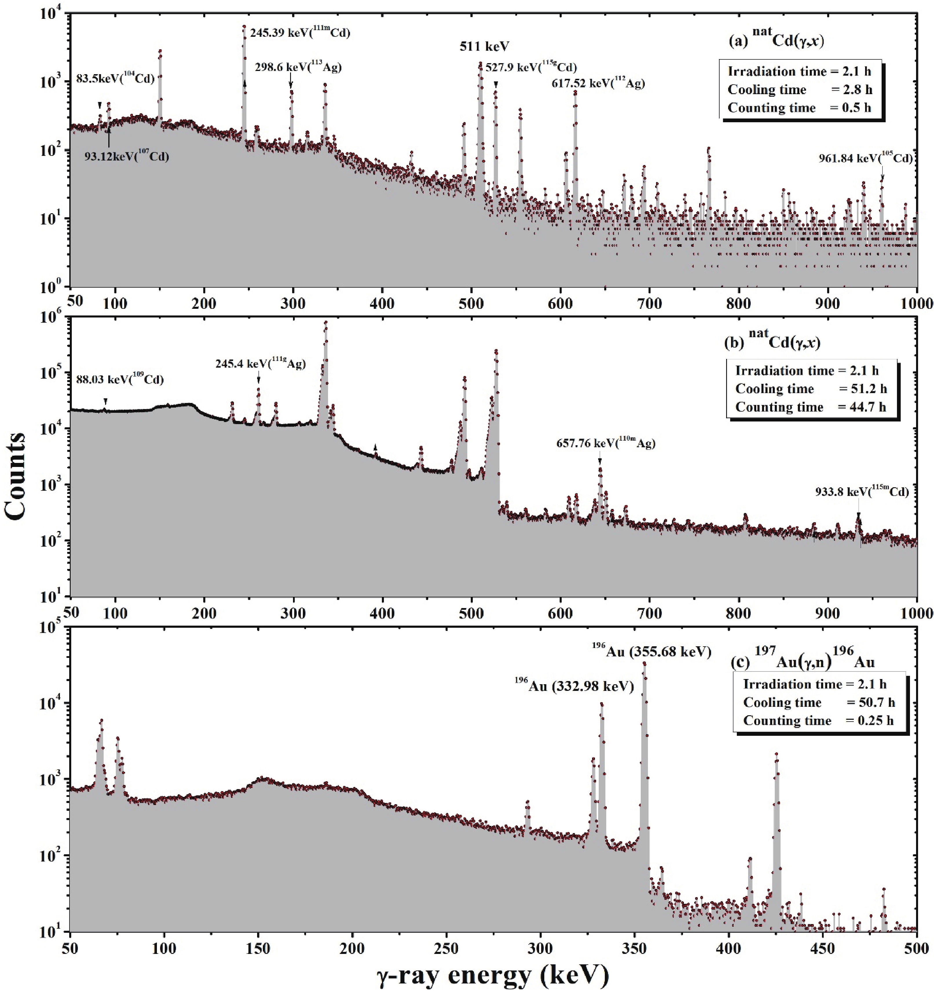
      Figure 1.  (color online) Typical γ-ray spectra of the products of the natCd(γ, x) reactions with cooling times of (a) 2.8 h and (b) 51.2 h, and (c) those of the 197Au(g, n) reaction with a cooling time of 50.7 h. The bremsstrahlung end-point energy used for the irradiation was 60 MeV.

      Nuclides (spin & parity) Half-life Decay mode (%) g-ray energy /keV γ-ray abundance (%) Reactions Q-value /MeV Threshold /MeV
      115gCd (1/2)+ 53.46 h β- : 100.00 336.24 45.9 116Cd(γ, n) −8.699 8.700
      Decay of 115mAg (T1/2 = 18 s) by β-(79%)
      527.90 27.45 Decay of 115gAg (T1/2 = 20 m) by β-(100%)
      115mCd (11/2)- 44.56 d β-: 100.00 158.03 0.02 116Cd(γ, n) −8.699 8.700
      484.47 0.29 Decay of 115Ag (T1/2 = 20 m) by β-(100%)
      933.80 2
      111mCd (11/2)- 48.5 m IT : 100 150.82 29.1 111Cd(γ, g’) 0.0 0.0
      112Cd(γ, n) −9.394 9.394
      113Cd(γ, 2n) −15.934 15.935
      245.39 94 114Cd(γ, 3n) −24.977 24.980
      116Cd(γ, 5n) −39.817 39.824
      109Cd (5/2)+ 461.9 d EC: 100 88.03 3.64 110Cd(γ, n) −9.915 9.915
      111Cd(γ, 2n) −16.891 16.892
      112Cd(γ, 3n) −26.285 26.288
      113Cd(γ, 4n) −32.824 32.829
      114Cd(γ, 5n) −41.867 41.875
      116Cd(γ,7n) −56.707 56.722
      107Cd (5/2)+ 6.5 h EC :100 93.12 4.7 108Cd(γ, n) −10.334 10.334
      110Cd(γ, 3n) −27.572 27.575
      111Cd(γ, 4n) −34.547 34.553
      112Cd(γ, 5n) −43.941 43.950
      828.93 0.163 113Cd(γ, 6n) −50.481 50.493
      114Cd(γ, 7n) −59.524 59.541
      116Cd(γ, 9n) −74.364 74.390
      105Cd (5/2)+ 55.5 m EC :100 346.87 4.2 106Cd(γ, n) −10.870 10.870
      108Cd(γ, 3n) −29.133 29.137
      433.24 2.81 110Cd(γ, 5n) −46.371 46.381
      111Cd(γ, 6n) −53.346 53.360
      961.84 4.7 112Cd(γ, 7n) −62.740 62.759
      113Cd(γ, 8n) −69.280 69.303
      104Cd (0)+ 57.7 m EC :100 106Cd(γ, 2n) −19.306 19.308
      66.6 2.4 108Cd(γ, 4n) −37.569 37.576
      83.5 47 110Cd(γ, 6n) −54.808 54.822
      709.3 19.5 111Cd(γ, 7n) −61.783 61.802
      112Cd(γ, 8n) −71.177 71.201
      113gAg (1/2)- 5.37 h β- : 100.00 258.72 1.64 114Cd(γ, p) −10.277 10.278
      116Cd(γ, p2n) −25.117 25.120
      298.6 10 Decay of 113mAg
      (T1/2 = 62 s, spin=7/2+) by IT(64%)
      Continued on next page

      Table 1.  Nuclear spectroscopic data of the products of the natCd(γ, xn), natCd(γ, pxn), and 197Au(γ, n) reactions. The photo-peak activities of γ-ray energies marked with bold letters were used for calculations.

    III.   DATA ANALYSIS

      A.   Determination of photon flux

    • The photon fluxes ({{\rm{\phi}} _{{E_{\rm e}}}}\left( {{E_\gamma }} \right)) as a function of photon energy (Eγ) for the bremsstrahlung spectra with electron beam energies (Ee) of 50 and 60 MeV were simulated using the GEANT4 code [23] and are shown in Fig. 2. The integrated photon flux \Phi \left( {{E_{\rm e}}} \right)\left( { = \int_{{E_{\rm th}}}^{{E_{\rm e}}} {{{\rm{\phi}} _{{E_{\rm e}}}}\left( {{E_\gamma }} \right){\rm d}{E_\gamma }} } \right) from the threshold to the electron beam energy was measured using the photo-peak activity of a 355.68 keV ( =87%) γ-line of 196gAu produced from the 197Au(γ, n)196gAu monitor reaction. The observed number of counts (N_{\rm obs}^{{E_{\rm e}}}) for the 355.68 keV γ-line of 196gAu was calculated by summing the counts under the full energy peak and subtracting the linear Compton back-ground, which is related to the integrated photon flux \Phi \left( {{E_{\rm e}}} \right) as follows [24]:

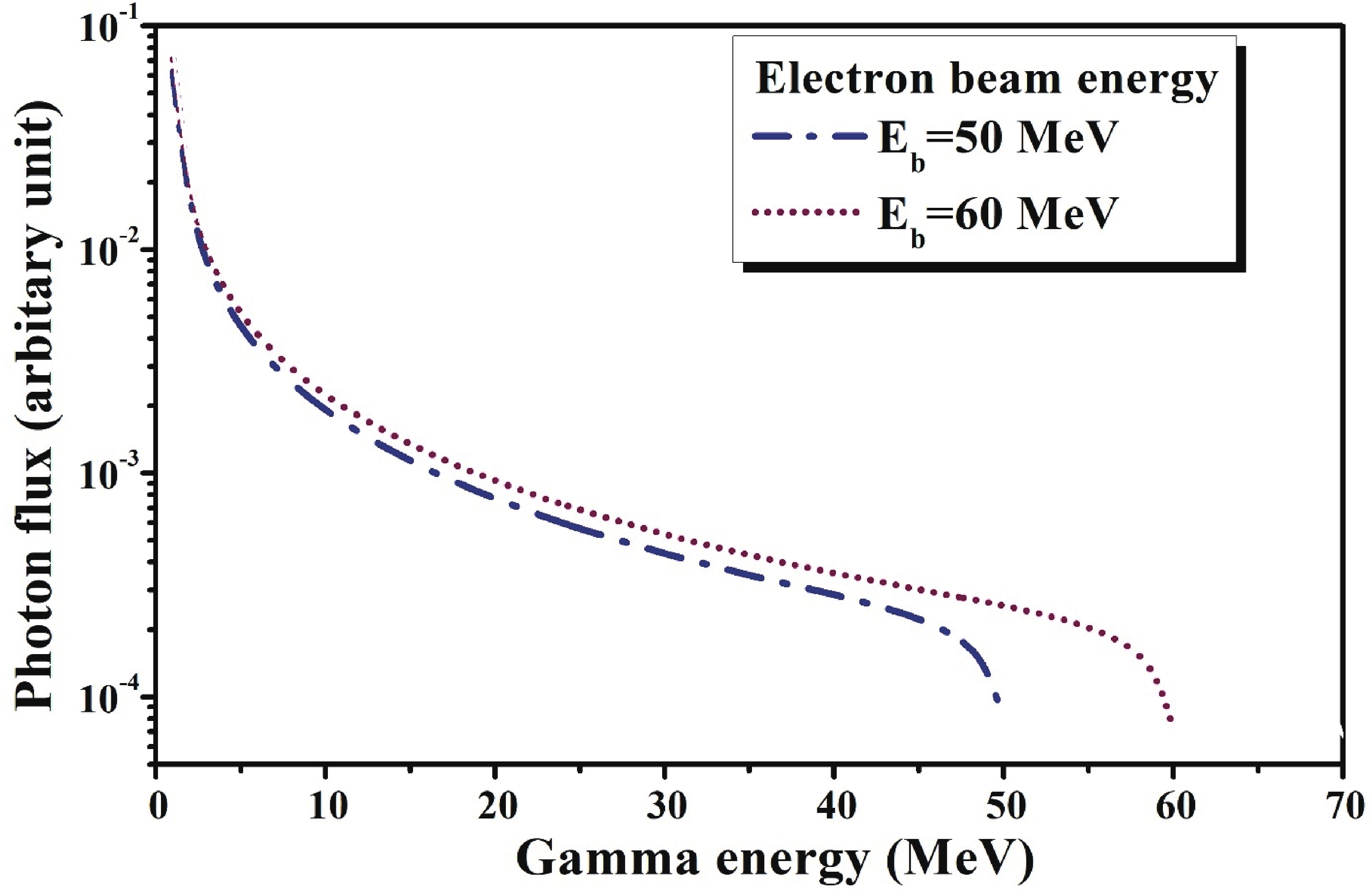
      Figure 2.  (color online) Typical bremsstrahlung spectra for the end-point energies of 50 and 60 MeV simulated using the GEANT4 code.

      \Phi \left( {{E_{\rm e}}} \right) = \frac{{N_{\rm obs}^{{E_{\rm e}}}\left( {CL/LT} \right)\lambda }}{{n\left\langle {{{\rm{\sigma}} _R}\left( {{E_{\rm e}}} \right)} \right\rangle {I_\gamma }{{\rm{\varepsilon}} _\gamma }\left( {1 - {{\rm e}^{ - \lambda {T_{\rm irr}}}}} \right){{\rm e}^{ - \lambda {T_{\rm C}}}}\left( {1 - {{\rm e}^{ - \lambda CL}}} \right)}},

      (1)

      where n and λ are the number of atoms in the flux monitor (Au) sample and the decay constant for 196gAu, respectively. Iγ and εγ are the branching intensity and detection efficiency of the selected γ-line, respectively. Tirr and TC, are the irradiation and the cooling times, respectively. CL and LT are the clock and live counting times, respectively. The detection efficiencies were measured using the standard calibration sources of 152Eu and 133Ba. \left\langle {{{\rm{\sigma}} _R}\left( {{E_{\rm e}}} \right)} \right\rangle is the known average cross section of the 197Au(γ,n)196gAu monitor reaction taken from Ref. [24], which is 103.3±12.1 mb and 102.4±9.5 mb for the bremsstrahlung end-point energies of 50 and 60 MeV, respectively. Nuclear data, such as the half-lives, γ-ray abundances, reaction Q-values, and threshold energies of the products, are given in Table 1 [21, 22].

      Table 1-continued from previous
      Nuclides (spin & parity) Half-life Decay mode (%) g-ray energy /keV γ-ray abundance (%) Reactions Q-value /MeV Threshold /MeV
      112Ag (2)- 3.13 h β- : 100.00 606.82 3.1 113Cd(γ, p) −9.749 9.749
      617.52 43 114Cd(γ, pn) −18.792 18.793
      694.87 2.9 116Cd(γ, p3n) −33.632 33.637
      111gAg (1/2)- 7.45 d β- : 100.00 245.40 1.24 112Cd(γ, p) −9.648 9.649
      113Cd(γ, pn) −16.188 16.189
      114Cd(γ, p2n) −25.231 25.234
      342.13 7 116Cd(γ, p4n) −40.071 40.079
      Decay of 111mAg (T1/2 = 1.08 m, spin=7/2+) by IT (99.3%)
      110mAg (6)+ 249.83 d IT : 1.33 657.76 95.61 111Cd(γ, p) −9.084 9.084
      112Cd(γ, pn) −18.478 18.479
      113Cd(γ, p2n) −25.018 25.021
      β- : 98.67 884.67 75 114Cd(γ, p3n) −34.061 34.066
      116Cd(γ, p5n) −48.901 48.912
      196gAu (2)- 6.18 d EC : 92.8 β- : 7.2 355.68 87.0 197Au(γ, n) −8.072 8.073
    • B.   Calculation of normalized yield and correction factor

    • Natural cadmium has eight stable isotopes with different isotopic abundances. The yield of the produced radionuclides is the sum of the isotope contributions based on their production threshold energies, as shown in Table 1. The eleven radio nuclides in Table 1 can be produced from natCd(γ, x)j reactions with different threshold values. The normalized yield contribution ({Y_{i,j}}\left( {{E_{\rm e}}} \right)) for each reaction of iCd(γ, x)j was obtained as follows [25]:

      {Y_{i,j}}\left( {{E_{\rm e}}} \right) = \frac{{\displaystyle\int_{{E_{\rm th}}}^{{E_{\rm e}}} {{A_i}\;{{\rm{\sigma}} _{i,j}}\left( {{E_\gamma }} \right){\rm{\phi}} \left( {{E_\gamma }} \right){\rm d}{E_\gamma }} }}{{\displaystyle\sum\limits_{k = 1}^8 {\int_{{E_{\rm th}}}^{{E_{\rm e}}} {{A_k}\;{{\rm{\sigma}} _{k,j}}\left( {{E_\gamma }} \right){\rm{\phi}} \left( {{E_\gamma }} \right){\rm d}{E_\gamma }} } }},

      (2)

      where i and k are eight stable isotopes (i, k = 106, 108, 110, 111, 112, 113, 114, 116) in natCd, and j is eleven produced isotopes (115g,m,111m,109,107,105,104Cd and 113g,112,111g,110mAg). {\rm{\phi}} \left( {{E_\gamma }} \right) is the photon flux calculated using the GEANT4 code [23], Ai(k) is the isotopic abundance, and {{\rm{\sigma}} _{i,j}}\left( {{E_\gamma }} \right) is the cross section for the iCd(γ, x)j reactions at the photon energy Eγ, which was calculated using the TALYS 1.95 code [17]. The normalized yield contributions for eleven radio isotopes j produced from various iCd(γ, x)j reactions are given in Table 2.

      Produced NucleiReactionEth/MeVE e =50 MeVEe =60 MeV
      {Y_{i,j}}\left( {{E_{\rm e}}} \right){F_{i,j}}\left( {{E_{\rm e}}} \right){Y_{i,j}}\left( {{E_{\rm e}}} \right){F_{i,j}}\left( {{E_{\rm e}}} \right)
      115gCd 116Cd(γ, n) 8.70 Y116,115= 100 F116,115= 0.934 Y116,115 = 100 F116,115= 0.940
      115mCd 116Cd(γ, n) 8.70 Y116,115= 100 F116,115= 0.934 Y116,115 = 100 F116,115= 0.940
      111mCd 111Cd(γ, g’) 0.0 Y111,111= 1.70 F111,111= 2.910 Y111,111 =1.40 F111,111= 2.710
      112Cd(γ, n) 9.39 Y112,111= 64.9 F112,111= 0.890 Y112,111=62.6 F112,111= 0.901
      113Cd(γ, 2n) 15.94 Y113,111= 18.5 F113,111= 0.554 Y113,111= 19.0 F113,111= 0.592
      114Cd(γ, 3n) 24.96 Y114,111= 14.5 F114,111= 0.306 Y114,111= 16.0 F114,111= 0.359
      116Cd(γ, 5n) 39.82 Y116,111= 0.40 F116,111= 0.080 Y116,111= 1.00 F116,111= 0.148
      109Cd 110Cd(γ, n) 9.92 Y110,109= 75.7 F110,109= 0.848 Y110,109= 74.1 F110,109= 0.863
      111Cd(γ, 2n) 16.89 Y111,109= 18.7 F111,109= 0.518 Y111,109= 18.7 F111,109= 0.560
      112Cd(γ, 3n) 26.29 Y112,109= 4.60 F112,109= 0.278 Y112,109= 5.00 F112,109= 0.333
      113Cd(γ, 4n) 32.83 Y113,109= 0.80 F113,109= 0.168 Y113,109= 1.10 F113,109= 0.231
      114Cd(γ, 5n) 41.86 Y114,109= 0.20 F114,109= 0.059 Y114,109= 1.10 F114,109= 0.127
      107Cd 108Cd(γ, n) 10.33 Y108,107= 67.5 F108,107= 0.823 Y108,107= 59.2 F108,107= 0.840
      110Cd(γ, 3n) 27.58 Y110,107= 24.7 F110,107= 0.255 Y110,107= 24.5 F110,107= 0.316
      111Cd(γ, 4n) 34.55 Y111,107= 7.30 F111,107= 0.145 Y111,107= 10.1 F111,107= 0.210
      112Cd(γ, 5n) 43.95 Y112,107= 0.50 F112,107= 0.039 Y112,107= 5.80 F112,107= 0.108
      113Cd(γ, 6n) 50.49 Y113,107= 0.00 F113,107= 0.00 Y113,107= 0.40 F113,107= 0.052
      105Cd 106Cd(γ, n) 10.87 Y106,105= 98.6 F106,105= 0.786 Y106,105= 96.4 F106,105= 0.806
      108Cd(γ, 3n) 29.14 Y108,105= 1.40 F108,105= 0.227 Y108,105= 1.60 F108,105= 0.286
      110Cd(γ, 5n) 46.38 Y110,105= 0.00 F110,105= 0.020 Y110,105= 1.90 F110,105= 0.086
      111Cd(γ, 6n) 53.36 Y111,105= 0.00 F111,105= 0.000 Y110,105= 0.10 F111,105= 0.033
      104Cd 106Cd(γ, 2n) 19.31 Y106,104= 98.2 F106,104= 0.443 Y106,104= 96.2 F106,104= 0.488
      108Cd(γ, 4n) 37.58 Y108,104= 1.80 F108,104= 0.107 Y108,104= 3.60 F108,104= 0.174
      110Cd(γ, 6n) 54.82 Y110,104= 0.00 F110,104= 0.000 Y110,104= 0.20 F110,104= 0.016
      113Ag 114Cd(γ, p) 10.28 Y114,113= 88.1 F114,113= 0.823 Y114,113= 92.9 F114,113= 0.840
      116Cd(γ, p2n) 25.12 Y116,113= 11.9 F116,113= 0.302 Y116,113= 7.10 F116,113= 0.356
      112Ag 113Cd(γ, p) 9.75 Y113,112= 27.0 F113,112= 0.862 Y113,112= 21.9 F113,112= 0.875
      114Cd(γ, pn) 18.79 Y114,112= 71.8 F114,112= 0.460 Y114,112= 74.3 F114,112= 0.505
      116Cd(γ, p3n) 33.64 Y116,112= 1.20 F116,112= 0.156 Y116,112= 3.80 F116,112= 0.234
      111Ag 112Cd(γ, p) 9.65 Y112,111= 56.9 F112,111= 0.862 Y112,111= 49.9 F112,111= 0.875
      113Cd(γ, pn) 16.19 Y113,111= 23.1 F113,111= 0.546 Y113,111= 23.0 F113,111= 0.585
      114Cd(γ, p2n) 25.23 Y114,111= 19.9 F114,111= 0.297 Y114,111= 26.5 F114,111= 0.352
      116Cd(γ, p4n) 40.08 Y116,111= 0.10 F116,111= 0.078 Y116,111= 0.60 F116,111= 0.146
      110mAg 111Cd(γ, p) 9.08 Y111,110= 17.5 F111,110= 0.905 Y111,110= 10.7 F111,110= 0.914
      112Cd(γ, pn) 18.48 Y112,110= 58.7 F112,110= 0.466 Y112,110= 49.2 F112,110= 0.511
      113Cd(γ, p2n) 25.02 Y113,110= 16.4 F113,110= 0.301 Y113,110= 18.3 F113,110= 0.356
      114Cd(γ, p3n) 34.06 Y114,110= 7.40 F114,110= 0.151 Y114,110= 21.6 F114,110= 0.215
      116Cd(γ, p5n) 48.91 Y116,110= 0.00 F116,110= 0.004 Y116,110= 0.20 F116,110= 0.065

      Table 2.  Normalized yield (%) and photon flux correction factor ({F_{i,j}}\left( {{E_{\rm e}}} \right)) for the iCd(γ, xn)j reactions.

      The threshold value (Eth) of the monitor reaction 197Au(γ, n)196Au is 8.07 MeV, as seen in Table 1. However, the production thresholds for the elevenradionuclides (j =115g,m;111m;109m,107m;105m;104mCd and 113g;112;111g;110mAg) are different from the monitor reaction as listed in Table 1. Therefore, a flux correction factor is required to correct the measured photon flux from the iCd(γ, x)j reactions to that from the monitor reaction. The photon flux correction factors {F_{i,j}}\left( {{E_{\rm e}}} \right) for iCd(γ, x)j were calculated as follows [25]:

      {F_{i,j}}\left( {{E_{\rm e}}} \right) = {{\int\limits_{E_{\rm th}^{i,j}}^{{E_{\rm e}}} {{\rm{\phi}} \left( {{E_\gamma }} \right){\rm d}{E_\gamma }} } \Big/ {\int\limits_{E_{\rm th}^{\rm Au}}^{{E_{\rm e}}} {{\rm{\phi}} \left( {{E_\gamma }} \right){\rm d}{E_\gamma }} }},

      (3)

      where i and j have the same definitions as in Eq. (2). E_{\rm th}^{i,j} and E_{\rm th}^{\rm Au} are the threshold energies for the iCd(γ, x)j and 197Au(γ,n)196gAu reactions, respectively. {\rm{\phi}} \left( {{E_\gamma }} \right) is the photon flux as a function of photon energy Eγ, taken from Fig. 2, which was simulated using the GEANT4 code [23]. The obtained correction factors to correct the different reactions to the monitor reaction are given in Table 2.

      The yield-weighted flux correction factors C_j^T\left( {{E_{\rm e}}} \right) for the jCd(γ, x)j reactions were calculated using Eqs. (2) and (3) as follows:

      C_j^T\left( {{E_{\rm e}}} \right) = {{\sum\limits_i {\left( {{Y_{i,j}}\left( {{E_{\rm e}}} \right) \times {F_{i,j}}\left( {{E_{\rm e}}} \right)} \right)} } \Big/ {\sum\limits_i {{Y_{i,j}}\left( {{E_{\rm e}}} \right)} }}.

      (4)

      The obtained yield-weighted flux correction factors C_j^T\left( {{E_{\rm e}}} \right) for the eleven produced isotopes (j) are listed in Table 3. The yield-weighted photon flux \Phi _j^C\left( {{E_{\rm e}}} \right) with the yield-weighted flux correction factors for the natCd(γ, x)j reactions were obtained as follows:

      Nuclear reactionsTotal correction factors (C_j^T\left( { {E_{\rm e}} } \right))
      Bremsstrahlung end-point energy, Ee/MeV
      5060
      natCd(γ, n)115gCd0.9340.941
      natCd(γ, n)115mCd0.9340.941
      natCd(γ, xn)111mCd0.7740.774
      natCd(γ, xn)109Cd0.7530.765
      natCd(γ, xn)107Cd0.6290.602
      natCd(γ, xn)105Cd0.7780.783
      natCd(γ, xn)104Cd0.4370.476
      natCd(γ, pxn)113gAg0.7610.806
      natCd(γ, pxn)112Ag0.5650.576
      natCd(γ, pxn)111gAg0.6760.665
      natCd(γ, pxn)110mAg0.4920.416

      Table 3.  Yield-weighted flux correction factor for the natCd(γ, x)j reactions.

      \Phi _j^C\left( {{E_{\rm e}}} \right) = C_j^T\left( {{E_{\rm e}}} \right) \times \Phi \left( {{E_{\rm e}}} \right).

      (5)
    • C.   Measurement of flux-weighted average cross sections

    • We determined the flux-weighted average cross sections using the yield-weighted photon flux \Phi _j^C\left( {{E_{\rm e}}} \right) for the natCd(γ, x)j reactions (the produced nuclei j is given as 115gm,111m,109,107,105,104Cd and 113g,112,111g,110mAg). The nuclear spectroscopic data for the reaction products were taken from Refs. [21, 22] and given in Table 1. Once the observed number counts under the photo-peak (N_{\rm obs}^{{E_\gamma }}) was acquired for the characteristic γ-ray energy of the produced radionuclide j, the flux-weighted average cross sections of the natCd(γ, x)j reactions were obtained as follows [25]:

      \left\langle {{\rm{\sigma}} _j^{\rm nat}\left( {{E_{\rm e}}} \right)} \right\rangle = \frac{{N_{\rm obs}^{{E_{\rm e}}}\left( {CL/LT} \right)\lambda }}{{n\Phi _j^C\left( {{E_{\rm e}}} \right){I_\gamma }{{\rm{\varepsilon}} _\gamma }\left( {1 - {{\rm e}^{ - \lambda {T_{\rm irr}}}}} \right){{\rm e}^{ - \lambda {T_C}}}\left( {1 - {{\rm e}^{ - \lambda CL}}} \right)}},

      (6)

      where all terms have the same meaning as in Eq. (1) and \Phi _j^C\left( {{E_{\rm e}}} \right) is the yield-weighted photon flux as given in Eq. (5).

    • D.   Theoretical calculations of flux-weighted average cross sections

    • The flux-weighted average cross sections were also theoretically calculated for all the residual nuclides of interest based on the TALYS 1.95 [17] and EMPIRE-3.2 Malta [18] nuclear codes and compared with the experimental data, which are presented in Table 4. The calculations based on TALYS 1.95 [17] and EMPIRE-3.2 Malta [18] were performed with their default parameters. The photon-induced reaction cross sections ({\rm{\sigma}} _R^x\left( {{E_i}} \right)) for the natCd(γ, x) reactions were calculated based on mono-energetic photons using the TALYS 1.95 [17] and EMPIRE-3.2 Malta [18] codes. In the calculations, all possible exit channels of the nuclear reactions of the given projectile energy were considered. The flux-weighted average cross sections \left( {\left\langle {{{\rm{\sigma}} _x}\left( E \right)} \right\rangle } \right) for the natCd(γ, x) reactions were calculated as follows:

      ReactionBremsstrahlung end-point energy/MeVFlux-weighted average cross-section \left\langle {{\sigma _i}} \right\rangle /mb
      Present workTheoretical calculations
      TALYS 1.95 [17]Empire 3.2 Malta [18]
      natCd(γ, xn)115gCd502.432 ± 0.3452.5213.631
      602.123 ± 0.2612.3303.544
      natCd(γ, xn)115mCd500.5 ± 0.0710.5340.778
      600.446 ± 0.0590.4930.760
      natCd(γ, xn)111mCd501.461 ± 0.2190.4580.811
      601.413 ± 0.2120.4490.785
      natCd(γ, xn)109Cd5012.346 ± 1.7869.0828.381
      6010.210 ± 1.5018.4667.724
      natCd(γ, xn)107Cd500.733 ± 0.1010.7880.656
      600.681 ± 0.0940.8340.711
      natCd(γ, xn)105Cd500.43 ± 0.0650.6690.702
      600.385 ± 0.0590.6320.651
      natCd(γ, xn)104Cd500.105 ± 0.0150.1210.112
      600.087 ± 0.0110.1120.086
      natCd(γ, xn)113g+mAg500.534 ± 0.0750.0570.108
      600.501 ± 0.0610.0570.110
      natCd(γ, xn)112Ag500.318 ± 0.0430.0680.159
      600.367 ± 0.0460.0810.172
      natCd(γ, xn)111g+mAg500.126 ± 0.0190.04250.121
      600.123 ± 0.0180.0450.119
      natCd(γ, xn)110mAg500.026 ± 0.0050.0170.032
      600.027 ± 0.0040.0260.035

      Table 4.  Flux-weighted average cross sections for the natCd(γ, xn) and natCd(γ, pxn) reactions.

      \left\langle {{\sigma _x}\left( E \right)} \right\rangle = {{\int\limits_{{E_{\rm th}}}^{{E_{\gamma \max }}} {\sigma _R^x({E_i})\;\varphi ({E_i}){\rm d}E} }\Bigg/ {\int\limits_{{E_{\rm th}}}^{{E_{\gamma \max }}} {\varphi ({E_i}){\rm d}E} }},

      (7)

      where \left({E}_{i}\right) is the bremsstrahlung photon flux as a function of energy (E) simulated by the GEANT 4 code [23], as shown in Fig. 2.

    IV.   RESULTS AND DISCUSSION
    • The measured flux-weighted average cross sections are presented in different figures along with theoretical calculations and previously published data. The numerical values of all the cross sections and the uncertainties are given in Table 4. As previously stated, natural cadmium has eight stable isotopes (116,114,113,112,111,110,108,106Cd). Thus, during irradiation, the production of a specific radionuclide is prone to contribution from many reaction channels based on the projectile energy.

      The overall uncertainties in the results were calculated by taking the square root of the quadratic sum of all independent statistical and systematic uncertainties [19]. The resulting statistical uncertainties were mainly contributed by the counting statistics from the observed number of counts under the photo-peak of each γ-line (1.5%~10.5%). This was estimated by accumulating the data for an optimum time that depends on the half-life of the produced nuclides. In contrast, the systematic uncertainties were calculated from the uncertainties of the flux estimation (~11.5%), the detector efficiency (~3%), the half-life of the reaction products (~2%), the distance between the sample and detector (~2%), the γ-ray abundance (~2%), the irradiation and cooling time (~2%), the current and electron beam energy (~1%), and the number of cadmium target nuclei (~0.3%). The total systematic uncertainty is approximately 12.58%. The overall uncertainty is found to be between ~12.67% and ~16.07%.

    • A.   Measured photo-nuclear reaction cross sections of cadmium isotopes

    • When natural cadmium is irradiated with bremsstrahlung radiation with end-point energies of 50 and 60 MeV, six cadmium isotopes are directly produced through natCd(γ, xn) reactions, except the 115g,mCd nuclides, which can be indirectly produced from the β- decay of 115g,mAg, as given in Table 1.

      In this study, the flux-weighted average cross sections of the natCd(γ, xn)115g,m,111m,109,107,105,104Cd reactions at the bremsstrahlung end-point energies of 50 MeV and 60 MeV are determined for the first time and presented in Table 4. All measurements of the produced cross sections of the cadmium isotopes are exclusive, that is, there is no contribution from any other short-lived radionuclides in the measurements. Even the 109,107,105,104Cd radionuclides have no isomers; hence, their reaction cross sections are also independent. For comparison, the cross sections for the reactions as a function of the mono-energetic photons were calculated using the TALYS-1.95 and Empire 3.2 codes with default parameters; the flux-weighted average cross sections were then calculated using Eq. (7).

    • 1.   natCd(γ, n)115g, 115mCd reaction
    • The radioisotope 115Cd is produced directly through the 116Cd(γ, n) reaction and indirectly through the β- decay of 115Ag. It has a short-lived ground state 115gCd (T1/2=53.46 h) and a long-lived meta-stable state 115mCd (T1/2=44.56 d). The simplified energy level and the decay scheme of 115m,gCd is shown in Fig. 3. The meta-stable state 115mCd with a half-life of 44.6 d decays directly to the ground state of 115In by the β- process with a branching ratio of 97%. Meanwhile, approximately 1.7% of the meta-stable state decays to the ground state of 115In (jπ=9/2+) through the excited state of 115In (jπ=7/2+) by emitting a 933.8 keV γ-ray. The unstable ground state 115gCd (jπ=1/2+) decays to the 336.24 keV state of 115In (Jπ = 1/2-) by a β- process with a branching ratio of 62.6%, which decays to the ground state of 115In (Jπ = 9/2+) via M4 transition by emitting a characteristic γ-ray of 336.2 keV. On the other hand, the unstable ground state 115gCd decays to the 864.1 keV state of 115In (J π = 1/2+) by a β- process with a branching ratio of 33.1%, which then decays to the 336.2 keV state of 115In (J π = 1/2-) by emitting a 527.9-keV γ-ray. In order to identify the 115m,gCd isomeric pairs, we used the 933.8 keV and 527.9 keV photo-peaks for the 115mCd and 115gCd nuclides, respectively. It is observed that both the metastable and ground states seem to be individual.

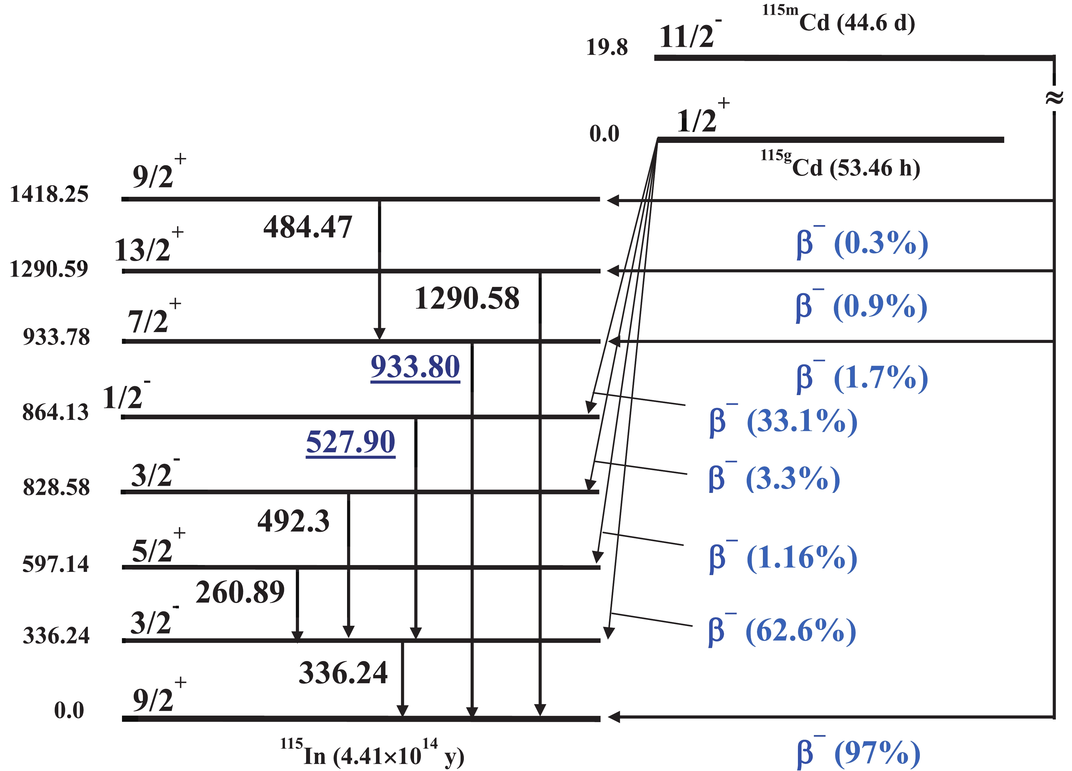
      Figure 3.  (color online) Simplified decay scheme of the 115g,,mCd isomers.

      The measured results for the natCd(γ, xn)115g;115mCd reactions are compared with the theoretical values obtained with the TALYS-1.95 and Empire 3.2 codes, as shown in Fig. 4. There is no literature data for the natCd(γ, xn)115gCd reaction. It is clear that the theoretical values from both the TALYS-1.95 and Empire 3.2 codes are in agreement with the data from this study, as shown in Fig. 4. However, there is only one set of literature data regarding the low energy side of the GDR region for the natCd(γ, xn)115mCd reaction [8], which was obtained with mono-energetic photons. To compare those results with the results of this study, we calculated the flux-weighted average cross section for the literature value using Eq. (7), as shown in Fig. 4. The flux-weighted average cross sections for literature data in the low energy region were higher than the theoretical results. However, the present results are lower than the values obtained with the TALYS-1.95 and Empire 3.2 codes, as shown in Fig. 4.

      Figure 4.  (color online) The experimental flux-weighted average cross sections of natCd(γ, xn)115gCd and natCd(γ, xn)115mCd reactions as a function of bremsstrahlung end-point energy along with the theoretical calculations using the TALYS-1.95 and EMPIRE-3.2 codes.

      Based on the measured experimental cross sections of the metastable and ground states from Table 4, we obtained the isomeric yield ratio (IR=σh/σl) of 115gCd (nuclear spin=1/2+) and 115mCd (nuclear spin=11/2-) in the natCd(γ, xn) reactions, which are given in Table 5 for various bremsstrahlung end-point energies. The photon-induced IR values from this study, the literature data in the GDR region [11-14], and our previous results [15] are listed in Table 5 and shown in Fig. 5. The IR values for neutron-induced 116Cd(n, 2n)115g,mCd reactions taken from previous data [16] and those theoretically calculated using TALYS-1.95, EMPIRE-3.2 Malta, and TENDL-2019 [26] are also presented in Table 5 and Fig. 5.

      ReactionProjectile energy/MeVExcitation energy/MeVIsomeric ratio ({IR} = { { {\sigma _{\rm HighSpin} } }/{\sigma _{\rm LowSpin} } })
      Experimental work [Ref.]Theoretical calculations
      TALYS 1.95 [17]Empire 3.2 Malta [18]
      natCd(γ, xn)115g,mCd5013.9220.206 ± 0.041 [A]0.2120.214
      6013.9280.210 ± 0.038 [A]0.2120.214
      116Cd(γ, n)115gmCd9.439.0720.180 ± 0.019 [12]0.0150.004
      116Cd(γ, n)115g,mCd2013.8030.117 ± 0.012 [14]0.2050.213
      116Cd(γ, n)115g,mCd2013.8030.148 ± 0.020 [11]0.2050.214
      116Cd(γ, n)115g,mCd2213.8410.120 ± 0.020 [13]0.2090.214
      116Cd(γ, n)115g,mCd23.513.8570.158 ± 0.016 [14]0.2090.214
      116Cd(γ, n)115g,mCd5013.9220.186 ± 0.020 [15]0.2120.214
      116Cd(γ, n)115g,mCd6013.9280.202 ± 0.020 [15]0.2120.214
      116Cd(γ, n)115g,mCd7013.9330.209 ± 0.019 [15]0.2120.214
      116Cd(n, 2n)115g,mCd13.419.040.95 ± 0.13 [16]1.3211.189
      116Cd(n, 2n)115g,mCd1419.640.98 ± 0.14 [16]1.3601.246
      116Cd(n, 2n)115g,mCd14.6820.321.0 ± 0.14 [16]1.3981.295
      116Cd(n, 2n)115g,mCd14.8120.451.05 ± 0.15 [16]1.4101.295
      116Cd(n, 2n)115g,mCd16.522.141.25 ± 0.18 [16]1.5101.364
      116Cd(n, 2n)115g,mCd17.9523.591.36 ± 0.19 [16]2.8102.690
      116Cd(n, 2n)115g,mCd19.7625.401.59 ± 0.22 [16]3.4613.101
      [A] Present work.

      Table 5.  Isomeric yield ratio of 115m,gCd from the 116Cd(γ, n) and 116Cd(n, 2n) reactions.

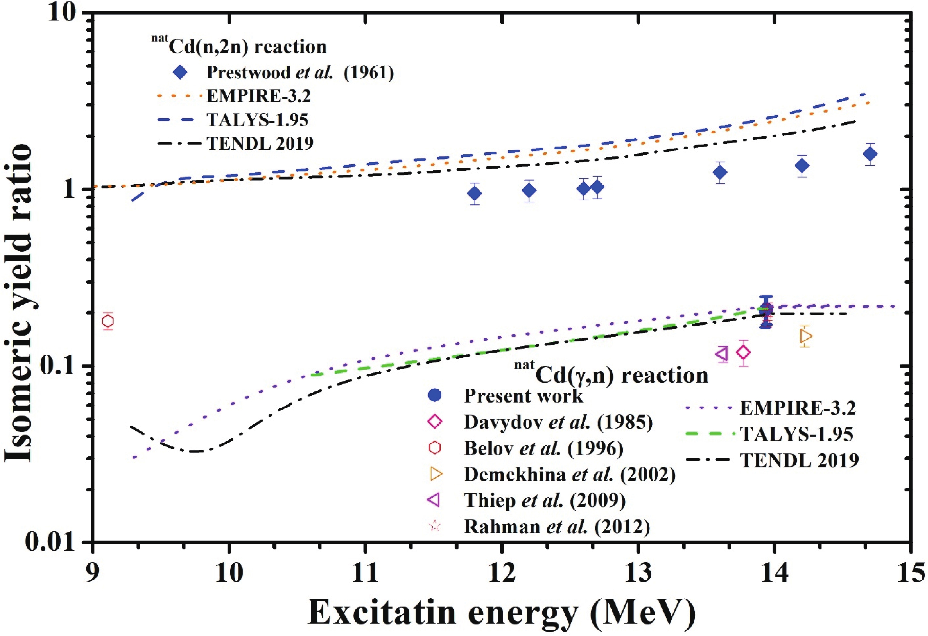
      Figure 5.  (color online) Isomeric cross section ratio (IR=σh/σl) of 115g,mCd in the (γ, n) and (n, 2n) reactions as a function of excitation energy of the compound nucleus.

      In order to understand the effects of spin and input angular momentum, outgoing particles, and excitation energy, the IR values from the different reaction channels were compared. The average excitation energy \left( {\left\langle {{E^*}\left( E \right)} \right\rangle } \right) of the compound nucleus from the threshold energy (Eth) to the bremsstrahlung end-point energy (Ee) was determined using the following expression [27, 28]:

      \left\langle {{E^*}\left( {{E_{\rm e}}} \right)} \right\rangle = \frac{{\int_{{E_{\rm th}}}^{{E_{\rm e}}} {{\rm{\phi}} \left( E \right){{\rm{\sigma}} _R}\left( E \right)E{\rm d}E} }}{{\int_{{E_{\rm th}}}^{{E_{\rm e}}} {{\rm{\phi}} \left( E \right)} {{\rm{\sigma}} _R}\left( E \right){\rm d}E}},

      (8)

      where {\rm{\phi}} \left( E \right) represents the photon flux as a function of photon energy (E) for the bremsstrahlung spectra, which was calculated using the Geant4 code, as shown in the Fig. 2. The reaction cross section ({{\rm{\sigma}} _R}\left( E \right)) was calculated using the default option in the TALYS-1.95 code. The calculated average excitation energies for the 116Cd(γ,n) reaction corresponding to different bremsstrahlung end-point energies are given in Table 5.

      The excitation energy (E*) of the compound nucleus in the neutron and charged particle induced reactions was calculated as follows:

      {E^*} = {E_{\rm p}} + \left( {{\Delta _{\rm T}}\, + \,{\Delta _{\rm p}}} \right)\, - \,{\Delta _{\rm CN}},

      (9)

      where Ep is the projectile energy, and {\Delta _{\rm CN}}, {\Delta _{\rm T}}, and {\Delta _{\rm p}} are the mass excess values of the compound nucleus, target, and projectile, respectively. The mass excess values are taken from the Nuclear Wallet Cards [29].

      As seen in Fig. 5, the experimental IR values in the 116Cd(γ, n) reaction are in agreement with the theoretical values. However, in the 116Cd(n, 2n) reaction, the theoretical values from TALYS-1.95, EMPIRE-3.2, and TENDL-2019 are higher than the experimental values. Additionally, in the 116Cd(n, 2n) reaction, the theoretical values from TALYS-1.95 and EMPIRE-3.2 are slightly different. TENDL-2019 data are lower than the TALYS-1.95 data but are close to the experimental data. These differences are due to the use of default parameters in the current calculations with TALYS-1.95. Furthermore, the figure shows that the IR values of 115m,gCd increase with increasing excitation energy. However, at the same excitation energy, the IR values of 115m,gCd in the 116Cd(n, 2n) reaction are significantly higher than those in the 116Cd(γ, n) reaction. In the 116Cd(γ, n) reaction, the compound nucleus is 116Cd*, which has a 0+ spin. On the other hand, in the 116Cd(n, 2n) reaction, the compound nucleus is 117Cd*, which has a 11/2- spin in the excited state and ½+ spin in the ground state. At a high excitation energy, the compound nucleus of 117Cd* with a high spin value of 11/2- will be favorable in the 116Cd(n, 2n) reaction. Thus, the high spin isomeric product 115mCd with a spin state of 11/2- will preferably be populated in the 116Cd(n, 2n) reaction, which results in a high IR value. This observation indicates the role of the spin of a compound nucleus alongside excitation energy. A similar observation can be made from our previous studies on the isomer ratio of 106m,gAg and 104m,gAg from the natAg (γ, xn) [30] and natAg(n, xn) [28] reactions, which support our present observations.

    • 2.   natCd(γ, xn)111mCd reaction
    • The isomeric state 111mCd (48.5 min, 11/2+) was identified by the pure and independent 245.39 keV γ-line. For the production of 111mCd from the 112Cd target, only two previous experimental data sets in the GDR energy region based on mono-energetic photons were available [8, 9]; these were found to be higher than the theoretical values obtained using the TALYS-1.95 and EMPIRE-3.2 Malta codes as shown in Fig. 6 and provided in Table 4. The figure and table also show that the current results follow the graphical shape but are higher than the theoretical values; they are the closest to the values calculated using the Empire-3.2 code.

      Figure 6.  (color online) Experimental flux-weighted average cross sections of the natCd(γ, xn)111mCd reaction as a function of bremsstrahlung end-point energy along with the theoretical calculations using the TALYS-1.95 and EMPIRE-3.2 codes.

    • 3.   natCd(γ, xn)109Cd reaction
    • The radionuclide 109Cd (461.9 d, 5/2+) was identified by the pure and independent 88.03 keV γ-line. The measured natCd(γ, xn)109Cd reaction cross-sections could onlybe compared with the theoretical calculations because no previous data has been found, as shown in Fig. 7 and tabulated in Table 4. In the figure, it is clear that the currently measured and theoretical values are in good agreement, in terms of not only shape but also magnitude.

      Figure 7.  (color online) Experimental flux-weighted average cross sections of the natCd(γ, xn)109Cd and natCd(γ, xn)107Cd reactions as a function of bremsstrahlung end-point energy along with the theoretical calculations using the TALYS-1.95 and EMPIRE-3.2 codes.

    • 4.   natCd(γ, xn)107Cd reactions
    • The flux-weighted average formation cross sections of 107Cd (6.5 h, 5/2+) were measured based on the 93.12 keV γ line. The measurements for the natCd(γ, xn)107Cd reaction were performed for the first time and thus could only be compared with the theoretical values. Fig. 7 shows that the measurements are in good agreement with both of the calculations, but they are closer to the EMPIRE-3.2 Malta calculations.

    • 5.   natCd(γ, xn)105Cd reactions
    • The flux-weighted average formation cross sections for 105Cd (55.5 min, 5/2+) were measured based on the independent 961.84 keV γ-line. The radioisotope (105Cd) is without an isomer. For this reaction, no literature data were available; hence, its measurements were also only compared with the theoretical calculations. In Fig. 8 and Table 4, it is clear that the flux-weighted average reaction cross sections calculated by the EMPIRE-3.2 Malta and TALYS-1.95 codes are almost the same, but they are higher than the currently presented results for the natCd(γ, xn)105Cd reaction.

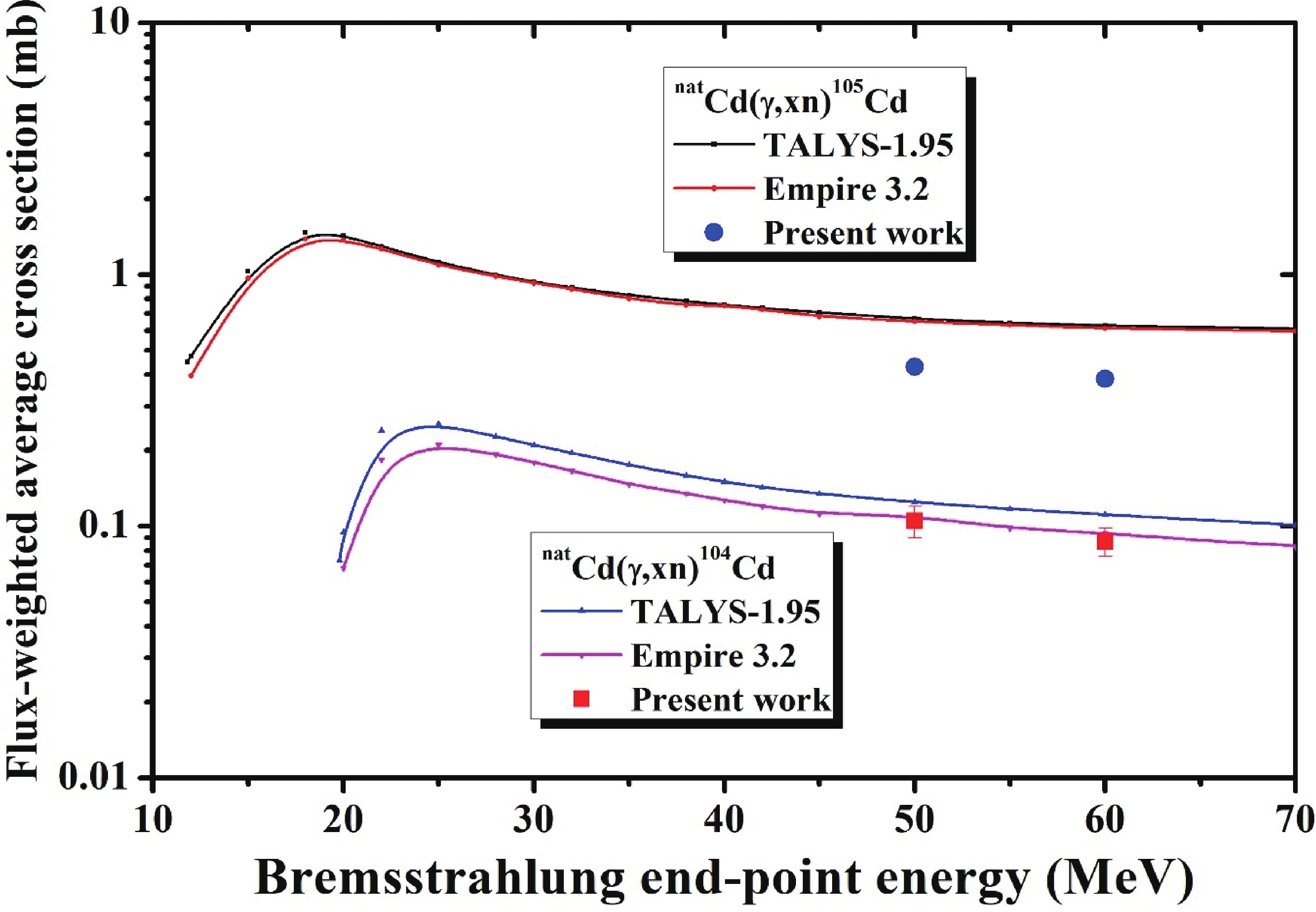
      Figure 8.  (color online) Experimental flux-weighted average cross sections of the natCd(γ, xn)105Cd and natCd(γ, xn)104Cd reactions as a function of bremsstrahlung end-point energy along with the theoretical calculations using the TALYS-1.95 and EMPIRE-3.2 codes.

    • 6.   natCd(γ, xn)104Cd reaction
    • The flux-weighted average formation cross section measurements of 104Cd (57.7 min, 0+) were also performed based onthe independent 83.5 keV γ-line. This reaction was studied for the first time and thus could only be compared with the theoretical values. In Table 4 and Fig. 8, the measured cross sections for the natCd(γ, xn)104Cd reaction are shown to be in good agreement with both calculations in terms of shape and magnitude, but they are more precisely matched with the EMPIRE-3.2 Malta calculations.

    • B.   Measured reaction cross-sections of silver radionuclides

    • Radioisotopes of silver (113g,112,111g,110mAg) were formed directly through (γ, pxn) reactions. During theirdirect production, 113gAg and 111gAg were populated by their short-lived metastable states by isomeric transition (IT). Therefore, their reaction cross sections were considered as cumulative values. 112Ag has no isomer, while 110mAg has no contribution from any other radioisotope for its production; hence, their formation cross sections are exclusive and independent. Further details on silver residual nuclides are given below.

    • 1.   Cumulative natCd(γ, pxn)113gAg reaction
    • The deduced cumulative formation cross sections of 113gAg (5.37 h, 1/2-) include the direct production and the production through decay of the short-lived isomeric state 113mAg (62 s, 7/2+), as presented in Fig. 9 and listed in Table 4. Measurements of the natCd(γ, pxn)113gAg reaction cross sections were performed using the 298.6 keV γ-line. Moreover, it is important to note that the production probability of the meta-stable state is low due to its high spin state (7/2+); therefore, we may conclude that 113mAg has a low contribution to the cumulative formation cross section of 113gAg. The measurements from the reaction were only compared with the theoretical values due to unavailability of published data. In Fig. 9(a), it is shown that the measured values for the reaction are higher than the calculated values; however, they exhibit the same tendency as the incident photon energy increases.

      Figure 9.  (color online) Experimental flux-weighted average cross sections of the (a) natCd(γ, x)113gAg and (b) natCd(γ, xn)112Ag reactions as a function of bremsstrahlung end-point energy along with the theoretical calculations using the TALYS-1.95 and EMPIRE-3.2 codes.

    • 2.   natCd(γ, pxn)112Ag reaction
    • The natCd(γ, pxn)112Ag reaction cross-sections were measured based on the 617.52 keV γ-line of 112Ag (3.13 h, 2-). This γ-line is also contributed to by 105Cd and 106mAg. However, after separating the contributions, it was found that their combined contribution to the 617.52 keV γ-line was only ~2%-3%, and thus, they were added to the photo peak area uncertainty. These measurements were only compared with the theoretical values due to unavailability of published data. In Fig. 9(b) and Table 4, the measured values are revealed to be higher than the calculated values; however, both follow a similar trend when the incident photon energy is increased. Moreover, the magnitude of the current measurements are shown to be closer to the EMPIRE-3.2 calculation than the TALYS calculation.

    • 3.   Cumulative natCd(γ, pxn)111gAg reaction
    • For measurements of the flux-weighted average production cross section of 111gAg (7.45 d, 1/2-), the situation is the same as in the previous case with (113gAg). It is formed directly via the (γ, pxn) reaction and through the IT (99.3%) decay of the simultaneously produced short-lived 111mAg (1.08 min, 7/2+). In this case,the nuclear spin of the metastable state is higher; hence, its production probability is lower than that of the ground state. Based on this, we may once again conclude that the cumulative cross section measurements of 111gAg have a low 111mAg decay contribution. A comparison of the present results with theoretical values is shown in Fig. 10(a) and Table 4.

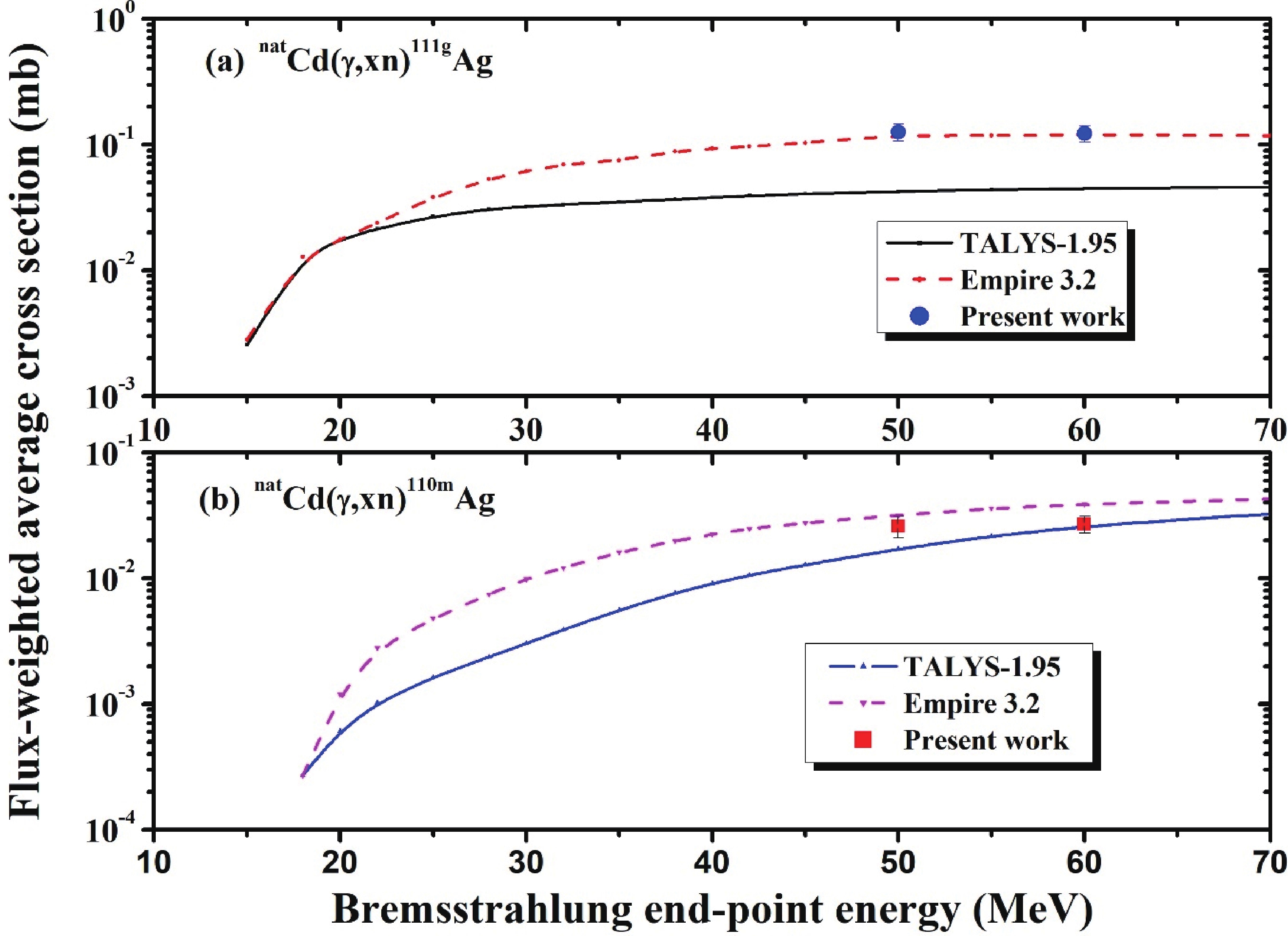
      Figure 10.  (color online) Experimental flux-weighted average cross sections of the (a) natCd(γ, xn)111gAg and (b) natCd(γ, xn)110mAg reactions as a function of bremsstrahlung end-point energy along with the theoretical calculations using the TALYS-1.95 and EMPIRE-3.2 codes.

    • 4.   natCd(γ, pxn)110mAg reaction
    • Flux-weighted average production cross sections of 110mAg (249.83 d, 6+) were measured based on the 657.76 keV γ-line. The gamma-ray spectrum was taken after sufficient time had passed to ensure other short-lived nuclides such as 105Cd, which contaminate the 657.76 keV γ-line, had sufficiently decayed. The measured results, along with the calculated values, are shown in Fig. 10(b) and listed in Table 4. Both of the results are consistent and higher than the theoretical values but closer to the values calculated using the EMPIRE-3.2 code.

    • C.   Integrated yield (Bq/g.μAh)

    • The production of cadmium and silver isotopes are important for medical and industrial applications and for a better understanding of their production in photon induced nuclear reactions. Therefore, the integrated yields (Bq/g.μAh) of cadmium and silver isotope productions from natCd(γ, x) reactions were measured in a procedure similar to that used for the integral yields of rhodium isotopes from the 103Rh(γ, x) reaction [19, 31]. The integral yields of cadmium and silver isotope productions from natCd(γ, x) reactions are given in Table 6.

      ReactionIsotopeYields/(Bq/g·A·h)
      Bremsstrahlung end-point energy/MeV
      5060
      natCd(γ, xn)115gCd115gCd(8.83±0.57)×106(8.52±0.60)×107
      natCd(γ, xn)115mCd115mCd(1.86±0.12)×106(1.80±0.19)×107
      natCd(γ, xn)111mCd111mCd(4.48± 0.28)×106(8.99±0.61)×107
      natCd(γ, xn)109Cd109Cd(3.62±0.26)×107(2.49±0.21)×108
      natCd(γ, xn)107Cd107Cd(1.71±0.12)×106(1.73± 0.12)×107
      natCd(γ, xn)105Cd105Cd(1.44±0.13)×106(1.17±0.14)×107
      natCd(γ, xn)104Cd104Cd(1.8±0.12)×105(1.73±0.15)×106
      natCd(γ, pxn)113g+mAg113m+gAg(1.58±0.11)×106(1.67±0.11)×107
      natCd(γ, pxn)112Ag112Ag(7.0±0.41)×105(8.74±0.53)×106
      natCd(γ, pxn)111g+mAg111gAg(3.3±0.24)×105(3.55±0.32)×106
      natCd(γ, pxn)110mAg110mAg(6.0±0.65)×104(5.6±0.40)×105

      Table 6.  Integral isotopic yield of different products from the natCd(γ, xn) and natCd(γ, pxn) reactions.

    V.   CONCLUSION
    • The flux-weighted average photon induced nuclear reaction cross-sections for the natCd(γ, xn; x=1-6)115g,m,111m,109,107,105,104Cd and natCd(γ, xnyp; y=1 x=1-5)113g,112,111g,110mAg reactions as well as the isomeric yield ratios of 115g,mCd in the 116Cd(γ, n) reaction were measured with the bremsstrahlung end-point energies of 50- and 60- MeV. Integral yield was also measured to assess the activities produced in the nuclear reactions. The photon induced formation reaction cross sections of natCd and the IR value of 115Cd were calculated using the TALYS-1.95 and EMPIRE-3.2 codes and the evaluated data taken from the TENDL-2019 library. In most of the cases, calculated values from the TALYS and EMPIRE codes matched each other and the experimental value. It was also found that the flux-weighted average cross sections increased sharply in the GDR region due to photo absorption and then decreased slightly in QDR region due to the opening of particle emission reaction channels. The isomeric yield ratio of 115g,mCd in the 116Cd(γ, n) reaction from this study and previously published data was compared with literature data for the 116Cd(n, 2n) reaction. It was found that the experimental IR values of 115g,mCd in the natCd(γ, xn) reaction agree with the calculations but were well below the IR values due to the 116Cd(n, 2n) reaction. The isomeric yield ratio previously measured in the 116Cd(n, 2n) reaction was lower than the calculated values for the same reaction; this is most likely due to the use of default parameters in the theoretical calculations. It was also observed that the theoretical and experimental values increased with excitation energy. However, at the same excitation energy, the IR values in the 116Cd(n, 2n) reaction were significantly higher than those in the 116Cd(γ, n) reaction due to the higher spin of the compound nucleus in the former. This indicates the role of compound nucleus spin alongside the effect of excitation energy.

    ACKNOWLEDGEMENT
    • The authors express their sincere thanks to the staff of the Pohang Accelerator Laboratory (PAL), Pohang, Korea, for the excellent operation and their support during the experiment.

Reference (31)

目录

/

DownLoad:  Full-Size Img  PowerPoint
Return
Return