


 Abstract
 HTML
HTML Reference
 Related
 PDF
PDF


-
Since 1998, when Riess et al. used SNIa data to statistically indicate that the expansion of universe is accelerating [1], physicists have been providing various theories to explain this acceleration, including the
$ f(R) $ theory [2], Brans-Dicke theory [3], and dark energy theory [4]. At present, the dark energy theory can be used to effectively explain the cosmic microwave background (CMB) anisotropies [5]; however, this study mainly focuses on the physical nature of dark energy. Dark energy can be studied using two main approaches. The first is to focus on the properties of dark energy, investigating whether or not its density evolves with time; this can be verified by reconstructing the equation of state$ w(z) $ for dark energy, which is independent of physical models. The reconstruction of the equation of state involves parametric and non-parametric methods [6], the latter including the Principal Component Analysis [7, 8], Gaussian Processes [9-11], PCA with the smoothness prior method [12-14], and PCA based on the Ridge Regression Approach [15]. The second involves dark energy physical models that are presented from the physical origin of its density and pressure, including scalar field models [16], preudo-Nambu-Goldstone bosons for cosmology [17], holographic dark energy [18], and age dark energy [19].Currently, it may be difficult to judge which model, method, or result is more persuasive; however, a model of dark energy that concerns its physical nature is essential. From the point of view of the models, Maziashvili presented a method that uses the Krolyhazy relation and time-energy uncertainty relation to estimate the density of dark energy [19, 20], and the result is consistent with astronomical data if the unique numerical parameter in the dark energy model is taken to be on the order of one.
Based on this, to further explore the origin of dark energy density and pressure, we present the possibility that dark energy density is derived from massless scalar bosons in a vacuum. If the scalar boson field is the radiation field that satisfies the Bose-Einstein distribution, positive pressure would be generated; hence, we first exclude this possibility based on the negative pressure of dark energy. Therefore, we can deduce the uncertainty in the position of scalar bosons based on the quantum fluctuation of space-time and the assumption that scalar bosons satisfy P-symmetry under a parity transformation, which can be used to estimate the scalar bosons and dark energy density.
-
The quantum fluctuation of space-time relates to the quantum properties of objects. Using the Heisenberg position-momentum uncertainty relations, Wigner derived a quantum limit on the measurability of a certain length [21]. If t is the time required by the measurement procedure, the uncertainty in the length measurement is
$ \delta t \sim \sqrt {\frac{t}{{{M_c}}}} , $

(1) where
$ {M_c} $ is the mass of the clock. We assume$ \hbar = c = 1 $ throughout this study.As a result of the above relation, when
$ {M_c} \to \infty $ ,$ \delta t \to 0 $ . To solve this situation, the quantum fluctuations of space-time itself is presented [22-25]. It also results in uncertainty in distance measurements. Thus, at very short distance scales, space-time is foamy, and the limitation of space-time distance measurements can be given by$ \delta t \sim \left\{ {\begin{array}{*{20}{l}} {{{({t_p}t)}^{\frac{1}{2}}}\;\;\;\;\;\;\;\;\;r > {t_p}}\\ {{t_p}\;\;\;\;\;\;\;\;\;\;\;\;\;\;\;\;r \leqslant {t_p}} \end{array}} \right. $

(2) where
$ {t_p} $ is the Planck time and$ {t_p} = \sqrt {\hbar G} $ . This limitation of space-time measurements can be interpreted as the result of quantum fluctuations of space-time. Meanwhile, Eq. (2) can be derived for massless particles in the framework of κ-deformed Poincare symmetries [26, 27].Krolyhazy derived another method for describing the quantum fluctuations of space-time, known as the Krolyhazy relation
$ \delta t \sim \;{t_p}^{2/3}{t^{1/3}}. $

(3) We consider that this quantum fluctuation effect is also applicable to the expanding universe. If the scalar boson field is the radiation field that obeys the Bose-Einstein distribution, positive pressure would be generated. Hence, we first exclude this possibility based on the negative pressure of dark energy. By assuming massless scalar bosons fall into the horizon boundary of the cosmos with the expansion of the universe, scalar bosons satisfy P-symmetry under the parity transformation, which can be expressed as
$ {P}\varphi ({r}) = - \varphi ({r}), $

(4) where
$ {\Psi _0} $ is the wave function of the scalar bosons. If$ r,t $ are the horizon size and age of the universe, from the P-symmetry and quantum fluctuation equations of space-time (2) or (3), the former can correlate the uncertainty in the relative position of two scalar bosons with the horizon size or age of the universe; hence, the uncertainty in the positions of scalar bosons is$ \delta {t_{\rm scalar}} \sim \delta t. $

(5) We hypothesise that the mean distance between scalar bosons is no less than the uncertainty relation
$\delta {t_{\rm scalar}}$ , and as a result, we obtain the number density of massless scalar bosons$ N = \delta {t^{ - 3}}. $

(6) If the quantum fluctuation of space-time provides scalar bosons with nonzero energy, we can consider the wave function
$ {\Psi _0} $ for the massless scalar bosons is non-stationary state. Its wavelength can be determined by the uncertainty relation$ \delta t $ ; hence,$ {\Psi _0} $ can be written as the superposition of at least n stationary states$ {\varphi _1},{\varphi _2},...,{\varphi _n} $ $ {\Psi _0} = \sum\limits_k^n {{\alpha _k}} {\varphi _k}{{\rm e}^{ -{\rm i}{w_k}t'}}, $

(7) where
${{w}_k} = 2\pi k/\delta t.$ It is easy to see that the state components$\varphi ,{{\rm e}^{-{\rm i}\omega {t'}}}$ are orthogonal in space and time, respectively.Alternatively, the wavelength of scalar bosons can be determined by the age of the universe t; hence, the wave function of scalar bosons
$ {\Psi _0} $ can be written as$ {\Psi _0} = \sum\limits_k^n {{{\bar \alpha }_k}} {\bar \varphi _k}{{\rm e}^{-{\rm i}{{\bar w}_k}t'}}, $

(8) where
${{\bar w}_k} = 2\pi k/t.$ The wave function$ {\Psi _0} $ will be further discussed using the Higgs potential or Yukawa interaction.By assuming scalar bosons or Goldstone bosons exist in a vacuum, Higgs proposed the existence of the Higgs scalar boson field, which can be described by the field equation [28]
$ {\nabla _\mu }{\nabla ^\mu }\Phi {\rm{ + }}{{{\rm{V}}}^\prime }(\Phi {\Phi ^*})\Phi = 0, $

(9) and when
$ \bar V'({\Phi _0}{\Phi _0}^*) = 0, $

(10) the massless-zero spin scalar boson field equation becomes
$ \Box {\Phi _0} = 0. $

(11) We consider this massless scalar field to contain zero-spin and zero-charge bosons and the scalar boson couples, or it undergoes Yukawa interaction with itself, which can be quantified in the simple potential energy form
$ - {f^2}{\Phi _0}{\Phi _0}^* $ , resulting in its massless state. If the Higgs singlet potential$ {\Phi _0} $ is substituted with the Yukawa potential U, the massless scalar bosons can interact with each other through propagator bosons provided they have weak isospins, which can be described by the Yukawa potential. Using Eq. (7) or (8), we incorporate a separation of the variable U$ U = {{U'}(r)}{{\rm e}^{-{\rm i}({w_k} - {w_l})t}}, $

(12) and the Yukawa potential
$ {U'}(r) $ satisfies$ \left\{ {\Delta - ({m_0}^2 - {w_{kl}}^2)} \right\}U' = - 4\pi g{\varphi _k}{\varphi _l}, $

(13) where
$ {w_{kl}} = {w_k} - {w_l} $ ,$ {m_0} $ is the mass of the Higgs or scalar boson, and g is the coupling constant. Solving the above equation yields$ {U'}(r) = g\int {\frac{{{e^{ - \mu \left| {r - {r'}} \right|}}}}{{\left| {r - {r'}} \right|}}{\varphi _k}({r'}){\varphi _l}({r'})} {\rm d} {r'}, $

(14) where
$ \mu = \sqrt {{m_0}^2 - {w_{kl}}^2} $ . -
When all scalar bosons are in the ground state
$ {\varepsilon _0} $ , that is$ {\varepsilon _0} = \delta {t^{ - 1}} \quad {\rm or} \quad {t^{ - 1}}, $

(15) we can use Eq. (2) or (3), (6), and (15) to obtain the internal energy per unit volume for massless scalar bosons
$ {{u = }}{\varepsilon _0}N \sim {({t_p}t)^{ - 2}}. $

(16) Next, we use the increase in entropy to derive the existence of negative pressure.
We consider the Boltzmann system to be composed of massless scalar bosons in vacuum; the bosons have a quantum state number
$ {W_p} $ for an energy level at the ground state$ {\varepsilon _0} $ , where$ {W_p} $ is considered the momentum degree of freedom. The momentum is$ {p_{{0}}} = \sqrt {\displaystyle\sum\limits_{{\rm{i = 1}}}^{{W_p}} {p_i^2} } $ . When$ {W_p} = 3 $ ,$ {p_{{0}}} = \sqrt {p_x^2 + p_y^2 + p_z^2} $ , and it is clear that the microstate numbers of the Boltzmann system are$ {3^N} $ ; hence, the system has statistical entropy per unit volume$ s = {k_B}\ln {3^N}, $

(17) where
$ {k_B} $ is the Boltzmann constant.Using the thermodynamic entropy definition
$T{\rm d}S = $ $ {\rm d} U + p{\rm d} V$ , where T is temperature, and the equations${\rm d}S = s{\rm d}V $ and${\rm d}U = u{\rm d}V$ with Eqs. (2), (6), (16), and (17), we get$ T = {(\ln {T_c})^{ - 1}}{k_B}^{ - 1}{({t_p}t)^{ - 1/2}}. $

(18) Because
$ u{({t_p}t)^2} $ is constant,$ {T_c} $ is also constant.We assume the degeneracy of energy
$ {W_p} $ is increasing gradually with the expanding universe, which can be expressed as$ {W_p}:1 \to 2 \to 3, $

(19) Hence, with the rise in
$ {W_p} $ , the entropy density will increase, which can generate negative pressure. From Eqs. (16), (17), and (19), we easily discover that the negative pressure$ {p_u} = {\omega _u}u $ satisfies$ T\ln {W_p}^N = (1 + {\omega _u})u, $

(20) and solving above equation yields
$ {\omega _u} = - 1 + \frac{{\ln {W_p}}}{{\ln {T_c}}}. $

(21) This is the equation of state for a scalar field in vacuum, and it contains an interesting feature. We set
$ {T_c} = 3 $ , and when$ {W_p} \to 1 $ , one has$ {\omega _u} \to - 1 $ ; if$ {W_p} \to 2 $ ,$ {\omega _u} \to - 1/3 $ . As a result, the vacuum energy moves from the ordered to disordered state with time and cannot violate the principle of entropy increase. In other words, negative pressure can be derived from the increasing entropy, which prevents the universe from maintaining expansion in the future. -
We assume that dark energy is composed of massless scalar bosons in vacuum, using Eq. (16), and obtain the dark energy density
$ {\rho _{de}} = {({t_p}t)^{ - 2}} $ . We introduce a numerical constant to ensure the equals sign satisfies Eq. (2) or (3), and choose the conformal time η as the time scale t [29, 30]. Hence, the energy density can be written as$ {\rho _{de}} = \frac{{3{n^2}{M_p}^2}}{{{\eta ^2}}}, $

(22) where
$ {M_p}^{ - 2} = 8\pi G $ ,$ {n^2} $ is the introduced numerical constant, and η is the conformal time, which is given by$ \eta = \int_0^t {\frac{{{\rm d}t}}{a}} , $

(23) where a is the scale factor of our universe. We take the present scale factor
$ {a_0} = 1 $ , and t is the age of the universe.Suppose the universe is spatially flat and the fraction of dark matter energy density is defined as
$ {\Omega _m} = {\rho _m}/3{M_p}^2{H^2} $ and$ {\Omega _{de}} = {\rho _{de}}/3{M_p}^2{H^2} $ ,$ {\Omega _m} = 1- {\Omega _{de}} $ is obtained from the Friedmann equation. Using Eq. (22),$ {\Omega _{de}} $ can be written as$ {\Omega _{de}} = \frac{{{n^2}}}{{{H^2}{\eta ^2}}} , $

(24) where
$ H = \dot a/a $ is the Hubble parameter. Using the energy conservation equation$ {\dot \rho _{de}} + 3H({\rho _{de}} + {p_{de}}) = 0 $ with Eqs. (22) and (24), the equation of state for the energy density$ {\omega _{de}} = {p_{de}}/{\rho _{de}} $ can be obtained as$ {\omega _{de}} = - 1 + \frac{2}{{3n}}\frac{{\sqrt {{\Omega _{de}}} }}{a} . $

(25) Meanwhile, using the Friedmann equations with equation Eq. (25) as well as
$ {\rho _m} \propto {a^{ - 3}} $ ,$ {\Omega _{de}} $ can be obtained, which satisfies [30]$ {\Omega '_{de}} = \frac{{{\Omega _{de}}}}{a}(1 - {\Omega _{de}})\left(3 - \frac{2}{n}\frac{{\sqrt {{\Omega _{de}}} }}{a}\right) , $

(26) where the prime represents the derivative with respect to
$ \ln a $ .This has some interesting features for the equation of state for dark energy. In the dark energy dominated phase, the energy density can drive the accelerated expansion of the universe if
$ {\omega _{de}} < - 1/3 $ . From Eq. (25), it is easy to see that when$ a \to \infty $ ,$ {\Omega _{de}} \to 1 $ ; thus,$ {\omega _{de}} \to - 1 $ at a later time. Moreover, in the matter dominated era,$ a \propto {t^{2/3}} $ , from Eqs. (22) and (23); thus,$ {\rho _{de}} \propto {a^{ - 1}} $ . Then, using the dark energy density conservation equation,$ {\omega _{de}} = - 2/3 $ can be obtained.At constant
$ {\omega _{de}} $ , the deceleration factor$ {q_0} $ is given by$ {q_0} = 0.5 + 1.5(1 - {\Omega _m}){\omega _{de}} $ ; we select$ {\Omega _m} = 0.3 $ of the current universe, which is taken from$\Lambda{\rm CDM}$ cosmology and SNIa Pantheon samples [31]. It is clear to see that when$ {\omega _{de}} \lesssim - 1/2 $ ,$ {q_0} < 0 $ , which implies that the energy density can drive the accelerated expansion of the universe if$ {\omega _{de}} \lesssim - 1/2 $ for the current universe.Moreover, we consider the case where the time scale t is replaced by the future event horizon
$ {R_h} $ , which was proposed by Li [18]. The future event horizon is$ {R_{\rm{h}}} = a\int_t^\infty {\frac{{{\rm d}t}}{a}} , $

(27) therefore, the dark energy density is
$ {\rho _{de}} = \frac{{3{n^2}{M_p}^2}}{{{R_h}^2}}. $

(28) By combining this with the dark energy density conservation equation, the equation of state for energy density can be given by [18]
$ {\omega _{de}} = - \frac{1}{3} - \frac{2}{{3n}}\sqrt {{\Omega _{de}}} . $

(29) At an earlier time, when
$ {\Omega _{de}} \to 0 $ ,$ {\omega _{de}} \to - 1/3 $ , and at a later time when$ {\Omega _{de}} \to 1 $ ,$ {\omega _{de}} \to - 1 $ for$ n = 1 $ . -
If we consider another case, where the expected energy value for scalar bosons
$ {\varepsilon _c} $ does not change with time,$ {\varepsilon _c} $ is constant; hence, Eq. (16) becomes$ u = {\varepsilon _c}\delta {t^{ - 3}}. $

(30) When we consider the dark energy density to be constrained by the expected value of the Higgs potential, Eq. (30) becomes more persuasive.
From Eq. (3), Eq. (30), and the introduction of the numerical constant
$ {n^2} $ , we obtain$ {\Omega _{de}} = \frac{{{n^2}}}{{t {H^2}}}. $

(31) Then, we can use the SNIa Pantheon sample and the Planck 2018 CMB angular power spectra to constrain the parameters of dark energy models, based on Eqs. (24) and (31).
-
In SNIa data, the Pantheon sample is a combination of SNe Ia data from Pan-STARRS1 (PS1), the Sloan Digital Sky Survey (SDSS), and SNLS as well as various low-z and Hubble Space Telescope samples. The Panoramic Survey Telescope & Rapid Response System (Pan-STARRS or PS1) is a wide-field imaging facility built by the University of Hawaii's Institute for Astronomy. It is used for a variety of scientific studies of the nearby to the very distant Universe and has provided 279 SNe Ia for the Pantheon sample [32]. The Supernova Legacy Survey Program detected approximately 2000 high-redshift Supernovae between 2003 and 2008, and the Pantheon sample contains approximately 236 SNe Ia, based on the first three years of data; these can be used to investigate the expansion history of the universe and improve the constraint of cosmological parameters as well as the study of dark energy [33].
In 2014, the SDSS Survey released a large catalogue containing the light curves, spectra, classifications, and ancillary data of 10,258 variable and transient sources [31, 34, 35-38]. The release generated the largest sample of supernova candidates, and 500 of this sample have been confirmed as SNe Ia by a spectroscopic follow-up. 335 SNe Ia in the Pantheon sample are taken from this spectroscopic sample. Others in the Pantheon sample are from the CfA
$ 1-4 $ , CSP, and Hubble Space Telescope (HST) SN surveys [33]. This extended sample of 1048 SNe Ia is called the Pantheon sample.Planck 2018 CMB angular power spectra data are based on observations obtained using Planck (http://www.esa.int/Planck), an ESA science mission with instruments and contributions directly funded by ESA Member States, NASA, and Canada.
-
When correcting the apparent magnitude of the Pantheon sample, considering the prior dark energy equation of state is unknown, we use SALT2 and a Taylor expansion of the
${{d}_H} - z$ relation to directly calibrate the distance modulus, which can simplify the problem.The Taylor expansion of the
${d_H} - z$ relation can be given by$\begin{aligned}[b] {d_{H,th}} = \frac{1}{{1 - y}}\left\{ y - \frac{{{q_0} - 1}}{2}{y^2} + \left[ {\frac{{3{q_0} - 2{q_0} - {j_0}}}{6} + \frac{{ - {\Omega _{{k_0}}} + 2}}{6}} \right]{y^3} \right\},\end{aligned} $

(32) where
$ y = z/(1 + z) $ . To reduce the calculation error of high redshift data, we use this variable substitution.$ {q_0} $ is the deceleration parameter,$ {j_0} $ is the jerk parameter, and$ {\Omega _{{k_0}}} $ is the curvature term.Meanwhile, the relationship between the distance modulus µ and luminosity distance
$ {d_H} $ can be written as$ \mu = 5{\log _{10}}{d_H} + 25 - 5{\log _{10}}{H_0}. $

(33) We use SALT2 and a Taylor expansion of the
${{d}_H} - z$ relation to directly calibrate the Pantheon sample. The distance modulus$ {\mu _{ob}} $ correction formula is given by the SALT2 model [39, 40]$ {\mu _{B,ob}} = {m_B} - {M_B}{\rm{ + }}\alpha \times {x_1}{\rm{ + }}\beta \times c{\rm{ + }}\Delta B, $

(34) where
$ {m_B} $ corresponds to the observed peak magnitude in the rest frame B band,$ {x_1} $ describes the time stretching of the light curve, c indicates the SN color at maximum brightness,$ \Delta B $ is a bias correction based on previous simulations, and α and β are nuisance parameters in the distance estimate.$ {M_B} $ is the absolute B-band magnitude, which depends on the host galaxy properties [31]. Notice that$ {M_B} $ is related to the host stellar mass (M stellar) by a simple step function$ {M_B} = \left\{ {\begin{array}{*{20}{l}} {M_B^1\;\;\;\;\;\;\;\;\;\;\;\;\;\;\;\;{\rm if}\;\;{M_{\rm stellar}} < {{10}^{10}}{M_ \odot }}\\ {M_B^1 + {\Delta _M}\;\;\;\;\;\;\;{\rm otherwise}} \end{array}} \right. $

(35) Here,
$ {M_ \odot } $ is the mass of the Sun.From Eqs. (33) and (34), the
$ {\chi ^2} $ of the Pantheon data can be calculated as$ {\chi ^2} = \Delta {\mu ^T}C_{{\mu _{ob}}}^{ - 1}\Delta \mu , $

(36) where
$ \Delta \mu = {\mu} - {\mu _{th}} $ .$ {C_\mu } $ is the covariance matrix of the distance modulus µ, and we only consider the statistical error$ \begin{aligned}[b] {C_{\mu,\rm stat}} = {V_{{m_B}}} + {\alpha ^2}{V_{{x_1}}} + {\beta ^2}{V_c} + 2\alpha {V_{{m_B},{x_1}}} - 2\beta {V_{{m_{B,c}}}} - 2\alpha \beta {V_{{x_1},c}}\, . \end{aligned} $

(37) From Eq. (36) combined with the Pantheon sample, we obtain the statistical average and error of the distance modulus µ and the parameters
$ {q_0} $ and$ {j_0} $ . Then, we use the calibrated Pantheon sample to constrain the dark energy model parameters. -
For model I, in which
$ {{\Omega }_{de}}={}^{{{n}^{2}}{{H}^{-2}}}\diagup{}_{t}\;$ , we first select the universe age T as the time scale t and consider a Taylor expansion of the$ T-z $ relation in near flat space to obtain$ T - {T_0} = - \frac{1}{{{H_0}}}\left(y - \frac{{{q_0}}}{2}{y^2} + \frac{{2{q_0}^2 - {j_0}}}{6}{y^3}\right), $

(38) where
$ {\rm{y}} = z/(1 + z) $ . To reduce the calculation error of the high redshift data, we use this variable substitution.$ {T_0} $ is the present age of the universe.Then, the Hubble parameter in near flat space can be written as
$ E(z) = \sqrt {{\Omega _m}{{(1 + z)}^3} + {\Omega _R}{{(1 + z)}^4} + \frac{{{n^2}}}{{T {H_0}^2}}} . $

(39) where
$E(z)={}^{H(z)}\diagup{}_{{{H}_{0}}}\;$ . From Eqs. (38) and (39),$ {{T}_{0}}={}^{{{n}^{2}}{{H}_{0}}^{-2}}\diagup{}_{(1-{{\Omega }_{m}})}\; $ when$ {\Omega _R} \ll {\Omega _m} $ .We use the
$ {\chi ^2} $ statistic fitting method to constrain the parameters as follows:$ {\chi ^2}_{\rm Pantheon} = \Delta {\mu ^T}{C_\mu }^{ - 1}\Delta \mu + \Delta {q_0}^2{\sigma _{{q_0}}}^{ - 2} + \Delta {j_0}^2{\sigma _{{j_0}}}^{ - 2}, $

(40) where
$ \Delta \mu = {\mu} - {\mu _{th}} $ .$\Delta {q_0} = {q_0} - {q_{0,\rm prior}}$ ,$\Delta {j_0} = {j_0} - {j_{0,\rm prior}}$ ,${q_{0,\rm prior}},\; {j_{0,\rm prior}}$ are given by the SALT2 calibration method in Section V.B.Following this, we combine Pantheon data with Eq. (39) to constrain the parameters and then use MCMC technology and the
$ {\chi ^2} $ statistic fitting method to obtain the statistical mean values and the minimum chi-square values without systematic errors of the parameters${\Omega _m},~ {n^2}{H_0}^{ - 1},~{q_0},~{j_0},~ {t_0}{H_0}$ , which are shown in Table 1. The confidence regions of the$ ({\Omega _m},{n^2}{H_0}^{ - 1}) $ plane are 68.3%, 95.4%, and 99.7%. (see Fig. 1)$ {{\Omega }_{\text{de}}}={}^{{{n}^{2}}{{H}^{-2}}}\diagup{}_{t}\; $ 

$ {\Omega _{\rm{m}}} $ 

$ {n^2}{H_0}^{ - 1} $ 

$ q_0 $ 

$ j_0 $ 

$ {t_0}{H_0} ({t_0} = {\eta _{{T_0}}}, {T_0}) $ 

$ \chi _{\min }^2/d.o.f. $ 

$ t = {\eta _T} $ 

0.23±0.013 3.3±0.5 −0.57±0.28 −0.2±2.7 4.3±0.7 1040/1050 $ t = T $ 

0.236±0.012 2.84±0.56 −0.44±0.31 −0.95±2.8 3.7±0.74 1044/1050 Table 1. Statistical mean values of the cosmological parameters from SN Ia Pantheon sample observation data combined with Model I.
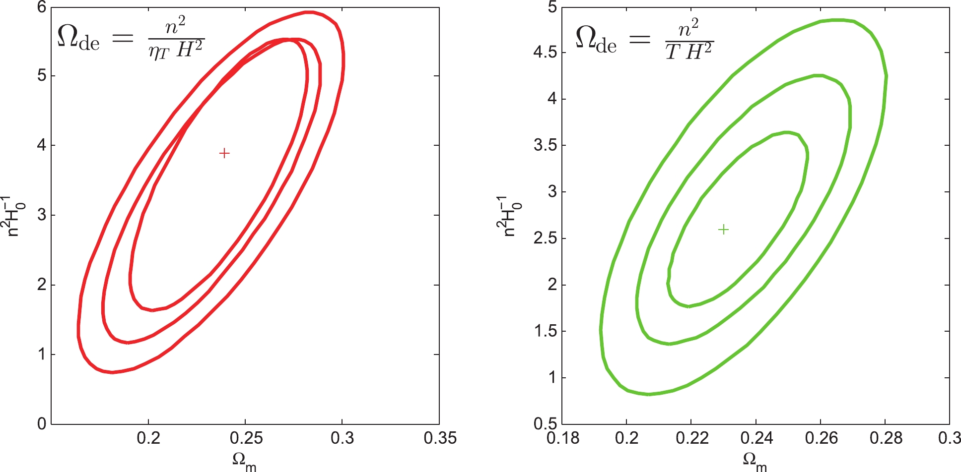
Figure 1. (color online) 68.3%, 95.4%, and 99.7% confidence regions of the (
${\Omega _m}$ ,${n^2}{H_0}^{ - 1}$ ) plane from Pantheon observation data combined with Model I. The + signs in their corresponding colors represent the best fitting values for${\Omega _m}$ and${n^2}{H_0}^{ - 1}$ .Moreover, we can select the conformal age
$ {\eta _T} $ as the time scale t and consider a Taylor expansion of the$ {\eta _T} - z $ relation in near flat space to obtain$ {\eta _T} - {\eta _{{T_0}}} = \frac{1}{{{H_0}}}\left\{ {y - \frac{{{q_0} - 1}}{2}{y^2} + \left[ {\frac{{3{q_0} - 2{q_0} - {j_0}}}{6}} \right]{y^3}} \right\}, $

(41) where
$ {\eta _{{T_0}}} $ is the currently conformal age of the universe.The Hubble parameter in near flat space can be expressed as
$ E(z) = \sqrt {{\Omega _m}{{(1 + z)}^3} + {\Omega _R}{{(1 + z)}^4} + \frac{{{n^2}}}{{{\eta _T} {H_0}^2}}} . $

(42) Then, from Eqs. (41) and (42),
$ {\eta _{{T_0}}} $ satisfies${{\eta }_{{{T}_{0}}}}= $ $ {}^{{{n}^{2}}{{H}_{0}}^{-2}}\diagup{}_{(1-{{\Omega }_{m}})}\;$ .Similarly, we use Eq. (42) with the Pantheon sample to fit the model parameters; the statistical results are shown in Table 1. Fig. 1 shows that the confidence regions of the
$ ({\Omega _m},{n^2}{H_0}^{ - 1}) $ plane are 68.3%, 95.4%, and 99.7%. -
When considering model II, in which
$ {{\Omega }_{de}}={}^{{{n}^{2}}{{H}^{-2}}}\diagup{}_{{{t}^{-2}}}\; $ , we can also select the universe age T as the time scale t, and the Hubble parameter in near flat space can be written as$ E(z) = \sqrt {{\Omega _m}{{(1 + z)}^3} + {\Omega _R}{{(1 + z)}^4} + \frac{{{n^2}}}{{T{ ^2}{H_0}^2}}} . $

(43) Alternatively, if we select the conformal age
$ {\eta _T} $ as the time scale t, the Hubble parameter in near flat space satisfies$ E(z) = \sqrt {{\Omega _m}{{(1 + z)}^3} + {\Omega _R}{{(1 + z)}^4} + \frac{{{n^2}}}{{{\eta _T}{ ^2}{H_0}^2}}} . $

(44) Using the pointing models Eqs. (43) and (44), we obtain statistical results for the parameters, which are shown in Table 2. Fig. 2 shows that the confidence regions of the
$ ({\Omega _m},n) $ plane are 68.3%, 95.4%, and 99.7%.$ {{\Omega }_{de}}={}^{{{n}^{2}}{{H}^{-2}}}\diagup{}_{{{t}^{2}}}\;$ 

$ {\Omega _m} $ 

n $ q_0 $ 

$ j_0 $ 

$ {t_0}{H_0} ({t_0} = {\eta _{{T_0}}}, {T_0}) $ 

$ \chi _{\min }^2/d.o.f. $ 

$ t = {\eta _T} $ 

0.19±0.016 4.4±0.44 −0.64±0.27 −1.1±2.6 5.5±0.62 1042/1050 $ t = T $ 

0.22±0.01 4.5±0.4 −0.48±0.3 −0.7±2.8 5.7±0.7 1044/1050 Table 2. Statistical mean values of the cosmological parameters from SN Ia Pantheon sample observation data combined with Model II.
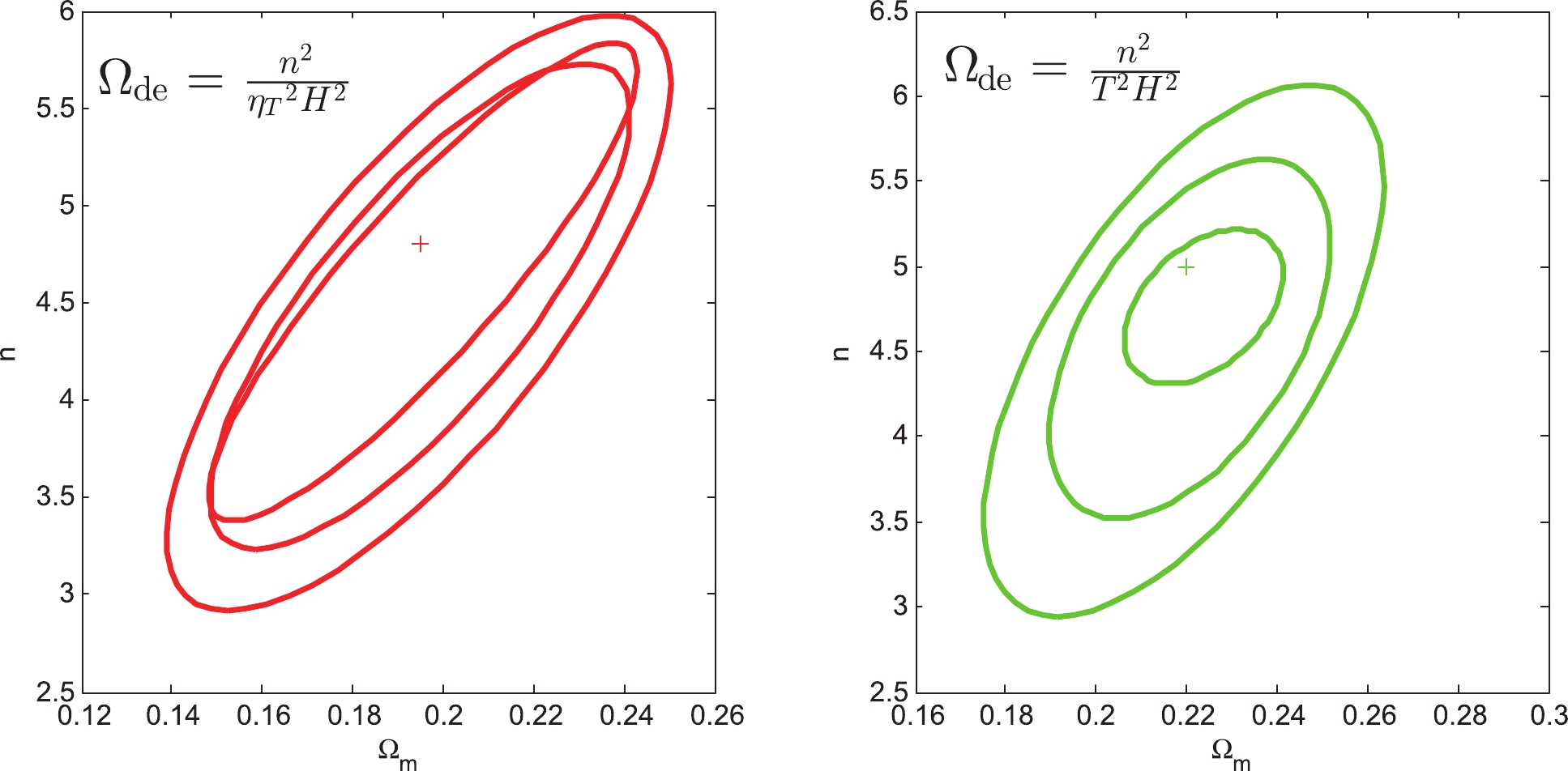
Figure 2. (color online) 68.3%, 95.4%, and 99.7% confidence regions of the (
${\Omega _m}$ , n) plane from Pantheon observation data combined with Model II. The + signs in their corresponding colors represent the best fitting values for${\Omega _m}$ and n.If we consider the current age of the universe to be
${T_0} = $ $ 13.5 \pm 0.5 \rm Gyr$ , which is inferred from globular clusters [41], the Hubble constant is${H_0} = 73.5 \pm 1.4\;{\rm{km }}\;\rm {s^{ - 1}} \; Mp{c^{ - 1}}$ using the NGC 4258 distance measurement [42]. By combining this with the fitting results obtained from the Pantheon sample, presented in Tables 1 and 2, we discover that selecting$ {\eta _T} $ as time scale may be more persuasive. Furthermore, for the mean value of$ {\Omega _m} $ , Conley et al. provided a statistical result of matter density for the constant$w{\rm CDM}$ model,$ {\Omega _m} = 0.19_{ - 0.10}^{ + 0.08} $ , from a combination of SNLS, HST, low-z, and SDSS data [33]. Our result is in agreement with this value.If only Pantheon data are used to investigate dark energy density, the statistical results indicate that the dark energy age models, including
$ {{\Omega }_{de}}={}^{{{n}^{2}}{{H}^{-2}}}\diagup{}_{{{\eta }_{T}}}\; $ and$ {{\Omega }_{de}}={}^{{{n}^{2}}{{H}^{-2}}}\diagup{}_{{{\eta }_{T}}^{2}}\;$ , have no evident superiority compared to$\Lambda {\rm CDM}$ using minimum chi-square. -
In addition, we can use Planck 2018 CMB angular power spectra data to constrain the model parameters. When
$ {\rm{z}} \geqslant 2.5 $ ,$ {}^{{{\Omega }_{m}}{{(1+z)}^{3}}}\diagup{}_{{{\Omega }_{de}}(z)}\;\gg 1 $ ; hence, we believe a Taylor expansion of the$ {\eta _T} - z $ relation is also applicable to calculate CMB angular power spectra. A calculation of$ C_{TT,l}^s $ that ignores the Sunyaev-Zeldovich (SZ) effect can refer to Weinberg 2008 [43], and the SZ-effect can refer to Bond et al. 2005 [44]. We use Planck 2018 data with Models I and II to constrain the cosmology parameters. The statistical mean values of the parameters are shown in Table 3, and Fig. 3 shows the CMB theoretical TT power spectra of the best fitting values from Planck 2018.$ {{\Omega }_{de}}={}^{{{n}^{2}}{{H}^{-2}}}\diagup{}_{{{\eta }_{T}}}\; $ 

$ {{\Omega }_{de}}={}^{{{n}^{2}}{{H}^{-2}}}\diagup{}_{{{\eta }_{T}}^{2}}\;$ 

$ {\Omega _b}{h^2} $ 

0.0214±0.00012 0.023±0.0002 $ {\Omega _c}{h^2} $ 

0.11±0.0014 0.107±0.0014 $ {10^{10}}{A_s}{e^{ - 2\tau }} $ 

1.29±0.016 1.316±0.027 $ {n_s} $ 

0.93±0.004 0.97±0.0025 ${N_{\rm eff} }$ 

3.45±0.13 3.5±0.35 $ {h_0} $ 

0.742±0.012 0.732±0.013 $ {\Omega _m} $ 

0.237±0.018 0.243±0.022 $ {n^2}{H_0}^{ - 1}, n $ 

5.5±0.33 4.85±0.54 $ q_0 $ 

−0.38±0.24 −0.7±0.59 $ j_0 $ 

1.3±0.22 4.7±1.2 $ \sigma _8^{sz} $ 

1.1±0.011 1.06±0.012 Table 3. Statistical mean values of the cosmological parameters from Planck 2018 TT power spectra data combined with Models I and II.
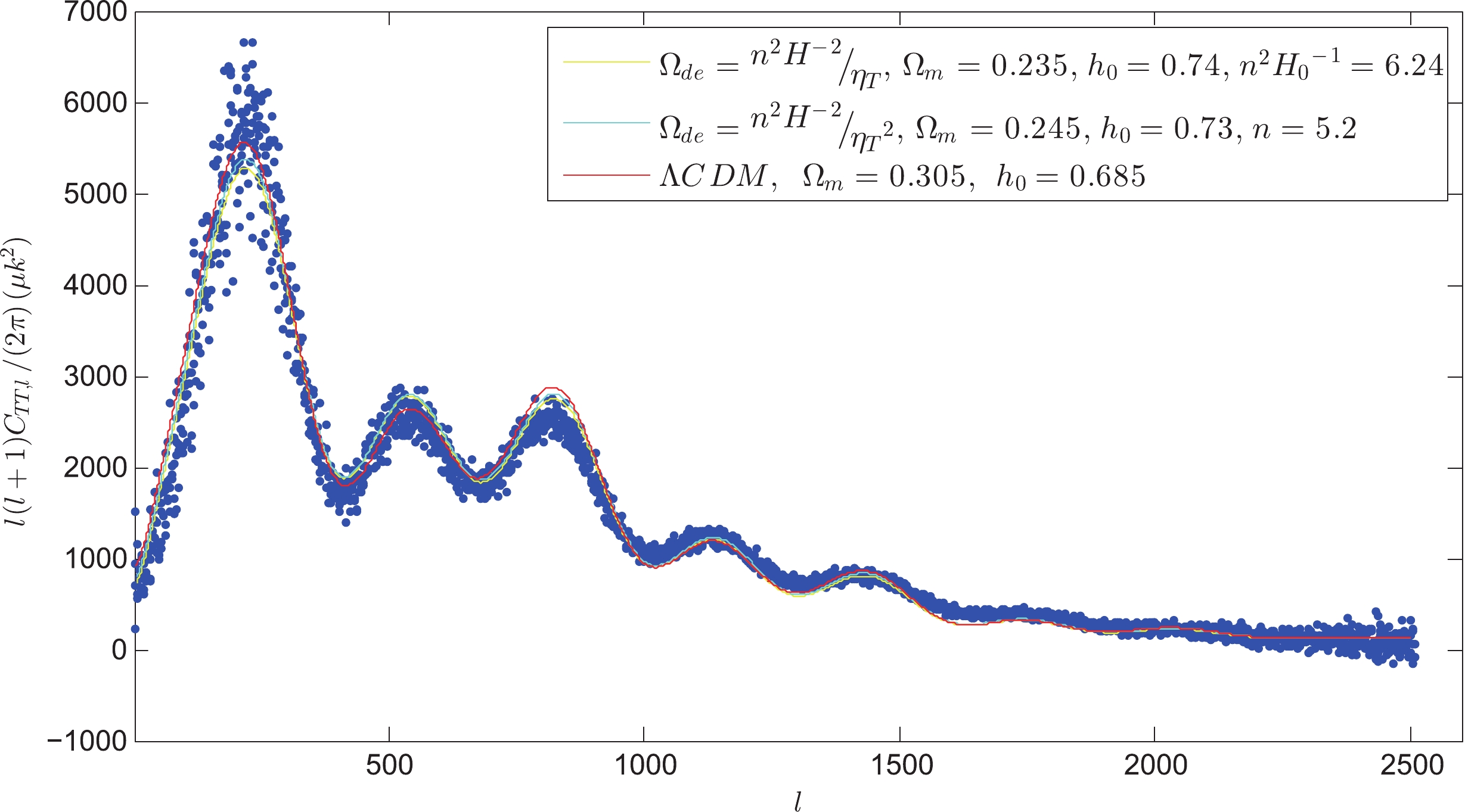
Figure 3. (color online) Blue dots represent Planck 2018 CMB TT angular power spectra. The red, yellow, and cyan lines are the CMB theoretical values of angular power spectra from
$\Lambda {\rm CDM}$ , Model I, and Model II, respectively, using the best fitting values, which are constrained by Planck 2018 data.In Table 3, we provide the statistical mean value of the Hubble constant
${H_0}{\rm{ = }}73.2 \pm 1.3\;{\rm{km}} \;\rm {s^{ - 1}} \; Mp{c^{ - 1}}$ , which is consistent with the result obtained using the NGC 4258 distance measurement [42].For the dark energy density, when using Planck 2018 CMB data, the statistical results indicate that the dark energy age models, including
$ {{\Omega }_{de}}={}^{{{n}^{2}}{{H}^{-2}}}\diagup{}_{{{\eta }_{T}}}\; $ and$ {{\Omega }_{de}}={}^{{{n}^{2}}{{H}^{-2}}}\diagup{}_{{{\eta }_{T}}^{2}}\; $ , have evident superiority, compared to$ \Lambda CDM $ using a minimum chi-square of$ l(l + 1)C_{TT,l}^s (l = 30 \sim 1500) $ . -
Understanding the physical nature of dark energy is important for our universe. In addition to the study of particle physics, dark energy may also enable us to further explore the nature of vacuum. Whether dark energy is derived from scalar bosons, other particles, or neither still needs to be further verified.
We explore a theoretical possibility that dark energy density is derived from massless scalar bosons in vacuum. Assuming massless scalar bosons fall into the horizon boundary with the expansion of the universe, scalar bosons satisfy P-symmetry under the parity transformation. P-symmetry with the quantum fluctuation of space-time enables us to estimate dark energy density. Meanwhile, to explain the physical nature of negative pressure, this is deduced from the increase in entropy density with the rise in degeneracy in the Boltzmann system.
Next, we used the SNIa Pantheon sample and Planck 2018 CMB angular power spectra to constrain the specified models. The statistical results indicate that the dark energy age models have evident superiority when using only CMB data compared to
$\Lambda{\rm CDM}$ using minimum chi-square. Furthermore, we obtain a statistical mean value of the Hubble constant${H_0}{\rm{ = }}73.2 \pm 1.3\;{\rm{km}} \;\rm {s^{ - 1}}\; Mp{c^{ - 1}}$ , which is consistent with the result obtained using the NGC 4258 distance measurement.Finally, we extend our discussion to the future of the universe. From Eq. (21), if
$ {W_p} $ satisfies$ {W_p}:3 \to 2 \to 1 $ , the universe may continue expanding in the future; however, if$ {W_p}:1 \to 2 \to 3 $ , this will change from expansion to contraction. Thus, the property of dark energy will dominate the future of the universe, and it will similarly determine the future of humanity.
Observational constraint on dark energy from quantum uncertainty
- Received Date: 2021-08-06
- Available Online: 2021-12-15
Abstract: We explore the theoretical possibility that dark energy density is derived from massless scalar bosons in vacuum and present a physical model for dark energy. By assuming massless scalar bosons fall into the horizon boundary of the cosmos with the expansion of the universe, we can deduce the uncertainty in the relative position of scalar bosons based on the quantum fluctuation of space-time and the assumption that scalar bosons satisfy P-symmetry under the parity transformation


 DownLoad: