


 Abstract
 HTML
HTML Reference
 Related
 PDF
PDF


-
The understanding of QCD matter at finite temperature and chemical potential is one of the main topics in theoretical physics. In recent decades, heavy-ion collision experiments, especially at the RHIC and LHC, have created a ground experiment environment for studying such matter. From the theoretical viewpoint, because the strong interaction coupling constant
$ \alpha_s $ is not small in most regimes, the perturbative method failed. Therefore, non-perturbative methods are needed to understand the physics in the large$ \alpha_s $ regime. One of the most useful tools is the Nambu-Jona-Lasinio (NJL) model [1, 2]. The NJL model has a long history dating back to 1961 (for reviews, see Refs. [3-5]); it incorporates chiral symmetry and its spontaneous breaking, and the gluonic degrees of freedom are replaced by a local four-point interaction of color currents. The essential point of this model is that it keeps the important symmetry in QCD, and it is trivial to represent the symmetry breaking in QCD, which is very useful for helping us understand the properties of QCD matter.Because of the point interaction used for quarks in the NJL model, the model is nonrenormalizable. Therefore, regularization should be used during the calculation. One of the fundamental problems is that when the temperature is finite, the contribution from the thermal part is convergent. It is an open question whether we need to use regularization on this part similar to that on the divergent vacuum part. Different choices not only change the numerical values of the results but also change the physical behaviors. A good example is given in Ref. [6], in which using/not using the regularization for the thermal part was discussed, and the dependence of the critical temperature on the chiral chemical potential gave two opposite results. On the one hand, the thermal part does not need a regularization as it is convergent, and to determine the full contribution from the thermal part, we should not use the regularization on this part. On the other hand, regularization should be applied to all parts of the equation to determine the correct physical quantities under the same energy limit for consistency. Therefore, to answer the question of the regularization of the thermal part, a systematic study is needed.
In this paper, we calculate the quark chiral condensate/quark constituent mass and grand potential related thermodynamics by using the framework of the two-flavor NJL model. We evaluate the physical quantities using three different regularization schemes and by introducing two different treatments for the thermal part for each scheme. We will investigate the simple and fundamental question: should we use regularization for the thermal part when we are using the NJL model to calculate the physical quantities?
-
The Lagrangian density of the two-flavor NJL model is given by
$ {\cal{L}} = \bar{\psi}({\rm i} \gamma_{\mu}\partial^{\mu} - m) \psi + G_S\left[(\bar{\psi}\psi)^2+(\bar{\psi}{\rm i}\gamma_5{{\tau}}\psi)^2\right]. $

(1) Here, m is the current quark mass,
$ {{\tau}} = (\tau^{1}, \tau^{2}, \tau^{3}) $ represents the isospin Pauli matrices, and$ G_{S} $ is the coupling constant with respect to the (pseudo)scalar channels. By using mean-field (Hartree) approximation the Lagrangian density can be given by [3],$ {\cal{L}} = -\frac{\sigma^2}{4 G_S} + \bar{\psi}({\rm i} \gamma_{\mu}\partial^{\mu} - M) \psi, $

(2) where the dynamical quark mass
$ \sigma = -2G_S\left<\bar{\psi} \psi\right> $ and$ \left<\bar{\psi} \psi\right> $ is the chiral condensate. Then, the constituent quark mass is given by$ M = m + \sigma $ . The general grand potential can be written for the vacuum part and the thermal part as follows:$ \Omega = \Omega_{\rm vac}+\Omega_{\rm th}, $

(3) where the vacuum and the thermal part are given by
$ \Omega_{\rm vac} = \frac{\sigma^{2}}{4G_{S}}-2N_f N_c \int \frac{{\rm d}^3 p}{(2\pi)^3}E_p({\boldsymbol{p}},M), $

(4) $ \begin{aligned}[b] \Omega_{\rm th} = &-2N_f N_c \int \frac{{\rm d}^3 p}{(2\pi)^3}T \\ & \times \left\{ \ln \left[1+ \exp\left(-\frac{E_p({\boldsymbol{p}}, M)-\mu}{T}\right)\right]\right. \\ & + \left.\ln \left[1+ \exp\left(-\frac{E_p({\boldsymbol{p}},M)+\mu}{T}\right)\right]\right\} . \end{aligned} $

(5) Here, the on shell energy of a quark is given by
$ E_p({\boldsymbol{p}},M) = \sqrt{{\boldsymbol{p}}^2 + M^2} $ .$ N_f $ and$ N_c $ are the numbers of the flavours and colors, which are 2 and 3, respectively, in this work. The constituent mass/chiral condensate can be solved by the corresponding gap equations$ \dfrac{\partial \Omega}{\partial \sigma} = 0 $ and$ \dfrac{\partial^2 \Omega}{\partial \sigma^2}>0 $ . It is easy to see that the integral for the vacuum part in Eq. (3) is divergent and the integral for the thermal part is convergent by integrating over the three momenta from 0 to infinity.In this study, we will use three different regularization schemes, (1) the three-momentum hard cutoff, (2) the three-momentum soft cutoff, and (3) the Pauli-Villas regularization. It should be mentioned here that the first two schemes are gauge covariant and the third one is gauge invariant.
Then, the vacuum part of the grand potential using regularizations can be written as
$ \Omega^{\rm H}_{\rm vac} = \frac{\sigma^{2}}{4G_{S}}-N_f N_c \int_0^{\Lambda} \frac{{\rm d} p}{\pi^2}p^2 E_p(p,M), $

(6) $ \Omega^{\rm S}_{\rm vac} = \frac{\sigma^{2}}{4G_{S}}-N_f N_c \int_0^{\infty} \frac{{\rm d} p}{\pi^2}f_{\Lambda}^2p^2 E_p(p,M), $

(7) $ \Omega^{\rm PV}_{\rm vac} = \frac{\sigma^{2}}{4G_{S}}-\sum\limits_{a = 0}^2 C_a \frac{N_f N_c}{\pi^2}\frac{M_a^4\ln M_a}{8}. $

(8) The thermal part when using regularizations is given by
$ \begin{aligned}[b] \Omega^{\rm H}_{\rm th} = &-N_f N_c \int_0^{\Lambda} \frac{{\rm d} p}{\pi^2}p^2 T \\ & \times \left\{ \ln \left(1+ \exp\left(-\frac{E_p(p,M)-\mu}{T}\right)\right)\right. \\ & + \left. \ln \left(1+ \exp\left(-\frac{E_p(p,M)+\mu}{T}\right)\right)\right\}, \end{aligned} $

(9) $ \begin{aligned}[b] \Omega^{\rm S}_{\rm th} = &-N_f N_c \int_0^{\infty} \frac{{\rm d} p}{\pi^2}p^2 f_{\Lambda}^2T \\ & \times \left\{ \ln \left(1+ \exp\left(-\frac{E_p(p,M)-\mu}{T}\right)\right)\right. \\ &+ \left.\ln \left(1+ \exp\left(-\frac{E_p(p,M)+\mu}{T}\right)\right)\right\}, \end{aligned} $

(10) $ \begin{aligned}[b] \Omega^{\rm PV}_{\rm th} =& -\sum\limits_{a = 0}^2 C_a \frac{N_f N_c}{\pi^2} \int_0^{\infty} \frac{{\rm d} p}{\pi^2}p^2 T \\ & \times \left[ \ln \left(1+ \exp\left(-\frac{E_p(p,M_a)-\mu}{T}\right)\right)\right. \\ & + \left.\ln \left(1+ \exp\left(-\frac{E_p(p,M_a)+\mu}{T}\right)\right)\right]. \end{aligned} $

(11) where the upper indexes H, S, and PV represent the hard cutoff, soft cutoff, and Pauli-Villas, respectively. The overall grand potential with different regularizations and that with/without applying the regularizations for the thermal part can be written as
$ \begin{aligned}[b] & \Omega^{\rm H} = \Omega^{\rm H}_{\rm vac} + \Omega^{\rm H}_{\rm th},\quad \Omega^{\rm H'} = \Omega^{\rm H}_{\rm vac} + \Omega_{\rm th},\quad \Omega^{\rm S} = \Omega^{\rm S}_{\rm vac} + \Omega^{\rm S}_{\rm th},\\& \Omega^{\rm S'} = \Omega^{\rm S}_{\rm vac} + \Omega_{\rm th},\quad \Omega^{\rm PV} = \Omega^{\rm PV}_{\rm vac} + \Omega^{\rm PV}_{\rm th},\quad \Omega^{\rm PV'} = \Omega^{\rm PV}_{\rm vac} + \Omega_{\rm th}, \end{aligned} $

(12) where the primes represent a regularization-free thermal part. The general parameters are given in Table 1. In addition, the soft cutoff weight function is chosen as
Regularization Scheme Λ/MeV m/MeV GS three-momentum hard cutoff 653 6 $2.14/\Lambda^2$ 

three-momentum soft cutoff 626.76 6 $2.02/\Lambda^2$ 

Pauli-Villas regularization 859 6 $2.84/\Lambda^2$ 

$ f_{\Lambda}(p) = \sqrt{\frac{\Lambda^{2N}}{\Lambda^{2N}+|{\boldsymbol{p}}|^{2N}}}, $

(13) here, we use
$ N = 5 $ . For the Pauli-Villas regularization, we set$ C_{a} = (1,1,-2) $ ,$ \alpha_a = (0, 2, 1) $ and$ M_{a}^2 = M^2 + \alpha_{a} \Lambda^2 $ for$ a = (0, 1, 2) $ , respectively.Also, we want to introduce the thermodynamic quantities, which depend on the grand potential directly in this work. The pressure is equal to the negative of the grand potential, i.e.,
$ P = -\Omega $ . By introducing the normalized grand potential, we will normalize the pressure at zero temperature and chemical potential equal to zero. Then, we have$ P(\mu, T) = \Omega(0, 0)-\Omega(\mu, T), $

(14) where
$ \Omega(0, 0) $ is the grand potential in vacuum. The energy density ϵ is given by$ \epsilon = -T^2\left. \frac{\partial(\Omega/T)}{\partial T}\right|_{V} = -T\left.\frac{\partial \Omega}{\partial T}\right|_{V}+\Omega-\Omega(0, 0), $

(15) and the corresponding specific heat is
$ C_{V} = \left.\frac{\partial \epsilon}{\partial T}\right|_{V} = -T\left.\frac{\partial^2 \Omega}{\partial T^2}\right|_{V}. $

(16) The square of the velocity of sound at constant entropy S is given by
$ v_s^2 = \left.\frac{\partial P}{\partial \epsilon}\right|_S = \left.\frac{\partial \Omega}{\partial T}\right|_V\bigg{/}\left.T\frac{\partial^2 \Omega}{\partial T^2}\right|_V. $

(17) -
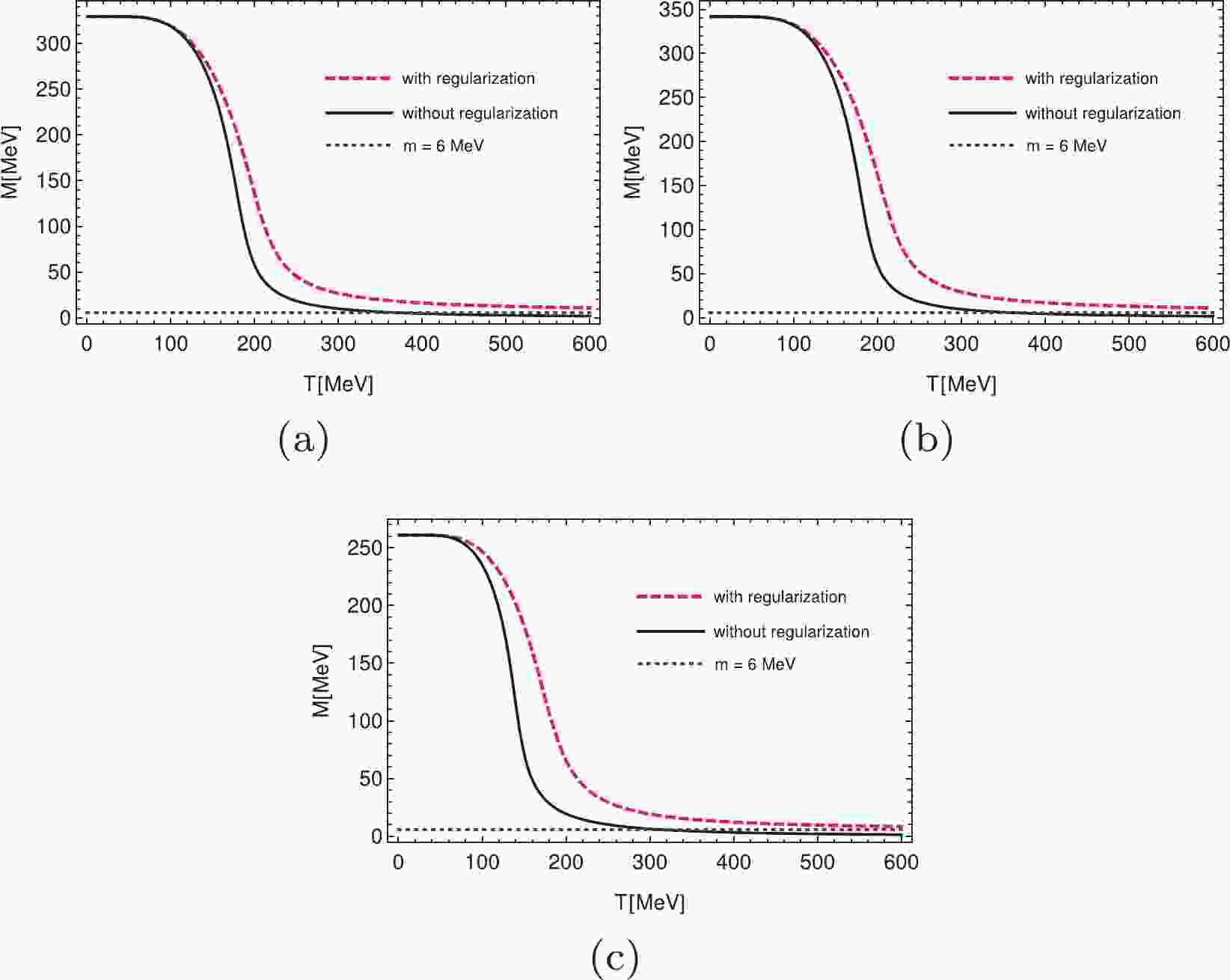
For simplicity, in the numerical calculations, we only consider the zero chemical potential case. It is obvious that the results should be equivalent to those from the finite chemical potential case. By solving the gap equation, we calculated the constituent mass of the quarks and several thermodynamical properties at zero chemical potential by using different regularizations. The constituent mass varies with the temperature with different regularization schemes, as shown in Fig. 1. It is shown, by using all three different regularization schemes, that the constituent quark mass is smaller than the current quark mass at high temperatures when regularizations are not used for the temperature part. Therefore, the chiral condensate is positive in this case, which is definitely an incorrect physical result. When we use the regularizations for the temperature part, the chiral condensate goes towards zero when the temperature increases. This means that the chiral symmetry is restored at high temperatures, which is physically correct. By definition, the constituent mass is always larger than the current mass in the framework of the NJL model, which has been mentioned in Ref. [5]. In fact, this is not a model dependent result. In the chiral limit, the chiral symmetry is an exact symmetry. The chiral condensate is negative in vacuum and increases to zero at some critical temperature. As the occurrence of chiral condensation is due to the dynamical effect, similar features should follow for the nonzero current quark mass, that is, the chiral condensate is always nonpositive at high temperatures. Furthermore, the change in the chiral condensate from a negative value through zero to a positive value would indicate that chiral symmetry is first restored and then broken again only by increasing the temperature. This certainly does not make sense.
Figure 1. (color online) Constituent quark mass as a function of temperature at zero chemical potential. For panels (a)-(c), the three momentum hard cut off, three momentum soft cut off and Pauli-Villas regularization are used, respectively. In all panels, the red dashed lines indicate that we use the regularization for the thermal part, the black solid lines indicate that we do not use the regularization for the thermal part, and the purple dotted lines indicate the current quark mass
$ m = 6$ MeV.In Figs. 2-4, we show the dimensionless quantities of pressure, energy density, specific heat, and the square of the sound velocity as a function of normalized temperature
$ T/T_0 $ for different regularization schemes (hard cutoff, soft cutoff, and Pauli-Villas regularization, respectively) at zero chemical potential in the NJL model.$ T_0 $ is the critical temperature at zero chemical potential; the values for using different regularization schemes are given in Table 2. By applying all three different regularization schemes, it is obvious that the behaviors when using and without using the regularizations for the thermal part are quite different for these quantities. It is well known that when the temperature increases, the thermal quantities should approach the results of the free Fermi gas. The most trivial quantity is the speed of sound, i.e.,$ v_s^2 = 1/3 $ at high temperature. When we are not using the regularizations for the thermal part, it is evident that the square of the speed of sound approaches this value at a high temperature, which is incorrect when we are using the regularizations for the thermal part because it is higher than the speed of light when the temperature is high. We have the same issue for other thermal quantities, regardless of the regularization we are using.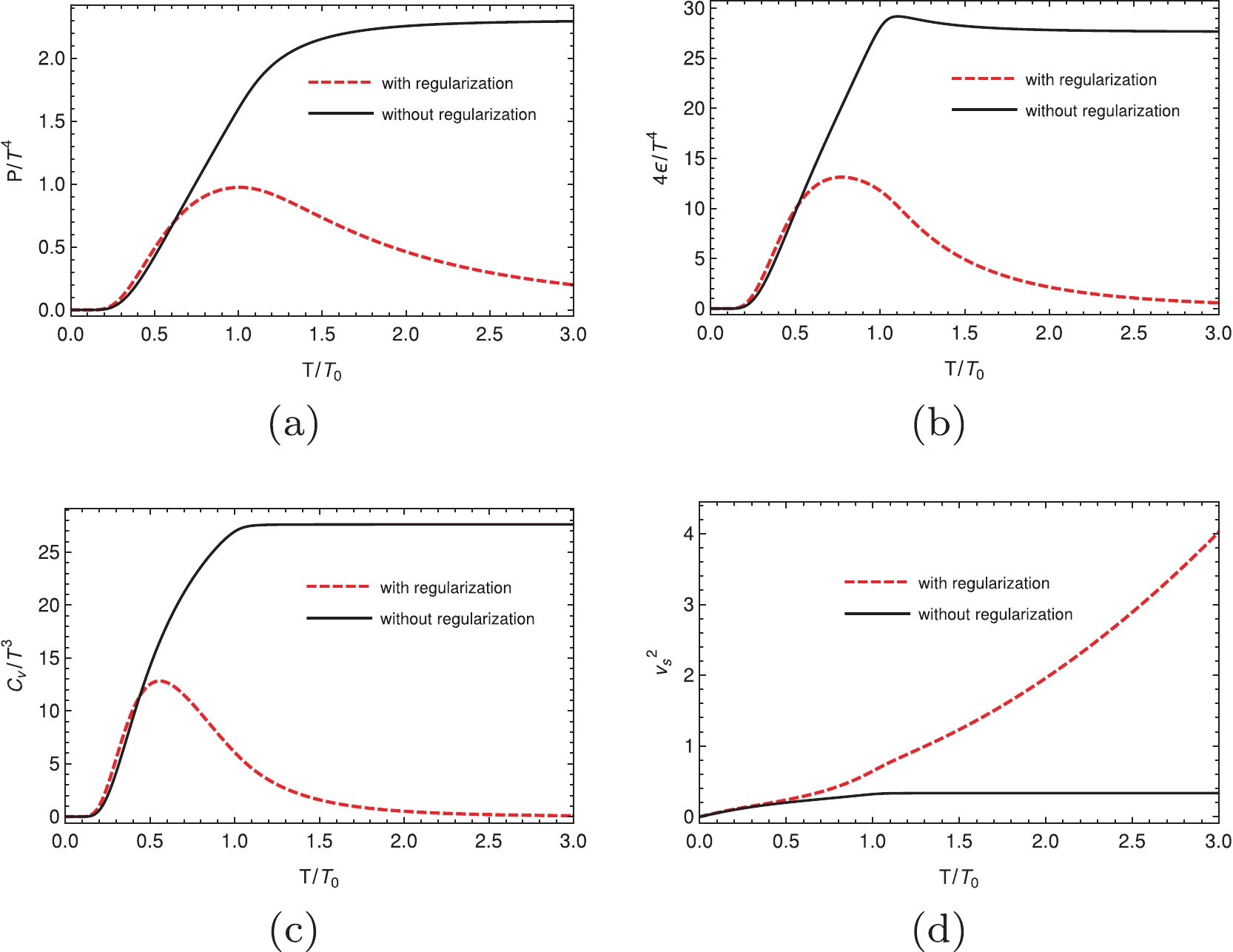
Figure 2. (color online) Dimensionless thermal properties as a function of the normalized temperature at zero chemical potential using the three momentum hard cutoff. In all panels, the red dashed lines indicate that we use the regularization for the thermal part, the black solid lines indicate that we do not use the regularization for the thermal part.
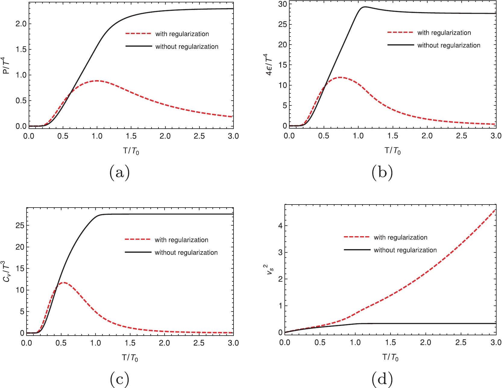
Figure 3. (color online) Dimensionless thermal properties as a function of normalized temperature at zero chemical potential using the three momentum soft cutoff. In all panels, the red dashed lines indicate that we use the regularization for the thermal part, the black solid lines indicate that we do not use the regularization for the thermal part.
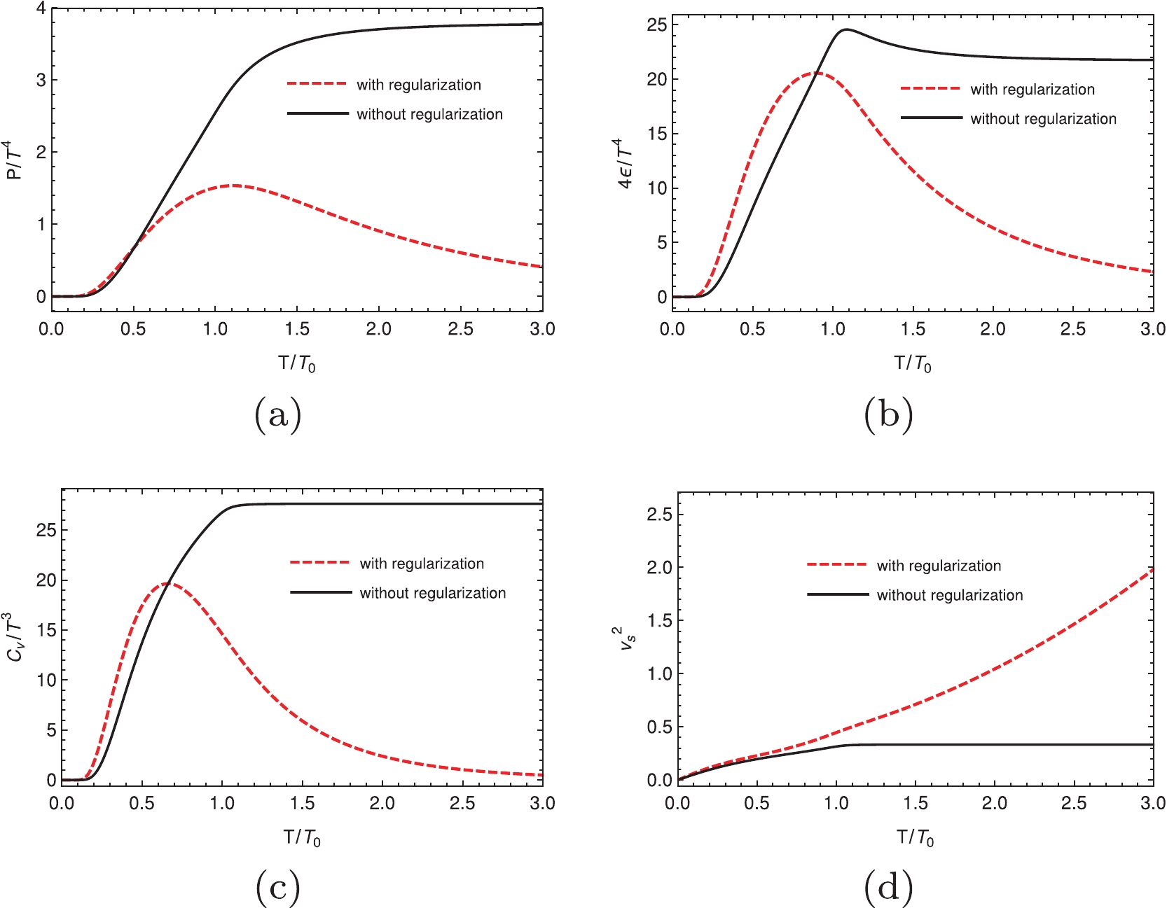
Figure 4. (color online) Dimensionless thermal properties as a function of normalized temperature at zero chemical potential using the Pauli-Villas regularization. In all panels, the red dashed lines indicate that we use the regularization for the thermal part, the black solid lines indicate that we do not use the regularization for the thermal part.
Regularization Scheme With/MeV Without/MeV three momentum hard cutoff 195 178 three momentum soft cutoff 202 179 Pauli-Villas regularization 172 138 Table 2. Values of
$T_0$ for different regularization schemes. “With” (“Without”) stands for using (not using) the regularization for the thermal part. -
In this paper, we discussed the fundamental question of whether we need to apply the regularization for the thermal part when we evaluate physical quantities in the NJL model by considering two sets of physical quantities: the chiral condensate and thermodynamical quantities, which are basically derived from the grand potential. By selecting a wide range of temperatures and three popular regularization methods (including both gauge covariant and gauge invariant schemes) in the NJL model, we find that to arrive at a physical result, we need to use (not use) the regularization for the thermal part when we are evaluating physical quantities related to the chiral condensate (grand potential). A good example is the net baryon fluctuation in QCD matter, which is very useful for studying the QCD phase transition. From the theoretical viewpoint, it purely depends on the orders of the derivative of the grand potential, for which we should not use the regularization for the thermal part, as can bee seen in one of the author's previous papers [8, 9]. In contrast, for some quantities, such as meson masses, which are directly related to the chiral condensate of quarks, we need to use the regularizations for the thermal part, e.g., Refs. [10, 11]. We could also come back to the question left in Refs. [6] which we mentioned in the introduction section. For calculating the chiral condensate and related chiral phase transition temperature, which are evaluated by the derivative of the chiral condensate, we need to use the regularization for the thermal part. Then, the behavior of the critical temperature and chiral condensate are consistent with the results from lattice QCD [12] and Dyson-Schwinger Equations [13]. A similar discussion about this specific problem is given in Ref. [14].
Another thing we want to mention here is that, although the numerical result is based on the simplest two flavor NJL model, it should be correct for all NJL based models because of model consistency. Also, we have covered the results for both gauge covariant and gauge invariant regularization schemes, and our conclusion should be valid for all other regularization schemes. Therefore, the results should help understand the physical qualities of QCD matter, especially in the non-perturbation regime. Also, this work should be very helpful for beginners, who are working on NJL based model projects.
Do we need to use regularization for the thermal part in the NJL model?
- Received Date: 2021-06-18
- Available Online: 2022-01-15
Abstract: The Nambu–Jona-Lasinio (NJL) model is one of the most useful tools for studying non-perturbative strong interactions in matter. Because it is a nonrenormalizable model, the choice of regularization is a subtle issue. In this paper, we discuss one of the general issues regarding regularization in the NJL model, which is whether we need to use regularization for the thermal part by evaluating the quark chiral condensate and thermal properties in the two-flavor NJL model. The calculations in this work include three regularization schemes that contain both gauge covariant and invariant schemes. We found that, regardless of the regularization scheme we choose, it is necessary to use regularization for the thermal part when calculating physical quantities related to the chiral condensate and to not use regularization for the thermal part when calculating physical quantities related to the grand potential.


 DownLoad: