


 Abstract
 HTML
HTML Reference
 Related
 PDF
PDF


-
Breakup reactions in nuclear physics have been shown to be the most appropriate mechanisms to probe the internal structure of halo-nuclei systems [1-3]. More recently, the intense experimental and theoretical activities undertaken by different groups on nuclear reactions with weakly-bound projectiles, as well as studies on the structure of halo-nuclei systems, can be traced from several reviews. These are exemplified by Refs. [4-8] reporting on recent developments in fusion and direct reactions with weakly-bound nuclei, and studies on the impact of nuclear forces on neutron-rich nuclei. Among the recent reviews, there are also studies considering exotic nuclei within the evolution of shell-model structure in Ref. [9]. The relevance of the studies on the structure and reactions with weakly-bound nuclei is associated with the fact that the fragmentation of the projectile into its constituents can provide a clearer picture on the halo-nuclei dynamics and structure, considering the interactions with the target nuclei via Coulomb and nuclear forces, leading to Coulomb and nuclear breakups respectively. Concerning related investigations in the last few years, we exemplify with those reported in Refs. [10-21], from which other relevant references can be obtained.
In spite of the amount of studies on both Coulomb and nuclear breakups, several questions remain. For example: How do the Coulomb and nuclear forces between projectile and target interfere to produce the total breakup? How can the total breakup be unambiguously separated into its Coulomb and nuclear components? Which one of the breakups, Coulomb or nuclear, is more affected by the couplings among the continuum states (continuum–continuum couplings)? Are there other factors apart from the target charge that can justify the importance of the Coulomb breakup over its nuclear counterpart in reactions involving a heavy target? Which of the forces, Coulomb or nuclear, produces a more prompt or delayed breakup? These questions may have related responses. However, definite answers will depend on many intrinsic or extrinsic parameters such as the incident energy, projectile breakup threshold, target mass, etc.
Another aspect, not less relevant, is the role of the nuclear interaction in the elastic scattering channel. It is often assumed that, since the breakup will occur in the asymptotic region, due to the projectile low breakup threshold, the nuclear interaction has a negligible effect, given its short-range nature. However, this remains to be established as a matter of fact, in view of the large size of a weakly-bound projectile wave function. Although the study of the nuclear interaction is apparently rather straightforward in the elastic scattering channel, it can be useful in probing some breakup dynamics. For instance, among others, it can expose in a specific way the dependence of the breakup process on the ground-state wave function. It may also serve to determine whether the breakup occurs asymptotically or in the “absorption region”, which is the region identified by laboratory angles θ larger than the “grazing angle” (the angle at which the elastic scattering trajectory starts to deviate from the Rutherford scattering) [22]. So, to estimate where the breakup process occurs, one can assess the amount of flux from the elastic scattering channel that reaches the absorption region. Furthermore, this may be helpful in better understanding the complete fusion process. On the other hand, the total fusion cross-section obtained in the Coulomb breakup, plus the nuclear interaction in the elastic scattering channel, might be interesting in the sense that it is not related to any sequential absorption of the fragments.
In the present study, our main goal is to analyze the relevance of the nuclear potential in the elastic scattering channel in the breakup of a loosely-bound neutron-halo projectile. For this purpose, we consider the breakup of the
$ s- $ wave neutron-halo 11Be nucleus on a lead target at an incident energy of 140 MeV, which is an incident energy of interest to due to the fact that experimental data became available very recently [23]. The effect of this nuclear potential on the total, Coulomb and nuclear breakup cross-sections will be investigated. In each breakup calculation, we will consider the cases where the continuum–continuum couplings are included in the coupling matrix elements, and when they are excluded. These couplings are known to strongly suppress the breakup cross-section (see for example Refs. [24-28] and references therein). Our expectation with this study is to shed more light on how the suppression occurs, by comparing the associated effect on the Coulomb and nuclear breakup cross-sections. One aspect of our investigation is to verify the importance of the projectile ground-state wave function on the breakup cross-sections. Associated with the total, Coulomb and nuclear breakups, we are also providing an estimation on the total fusion cross-sections, with an emphasis on the Coulomb breakup case, where no sequential absorption effect exists. By comparing the different fusion cross-sections, one can estimate the contribution of the off-diagonal absorption to the total fusion cross-section.By considering that all the breakup cross-sections are obtained by using the continuum discretized coupled-channel (CDCC) formalism [29, 30], the methodology adopted in this work consists of three different calculations for each type of breakup reaction:
$ {\bf{(i)}} $ When the nuclear potential in the elastic scattering channel is obtained by folding the potentials between target and fragments with the projectile ground-state wave function;$ {\bf{(ii)}} $ When the nuclear potential in the elastic scattering channel is obtained from the global parametrization of Akyüz and Winther [31] (similar to the one which is used in a single channel calculation);$ {\bf{(iii)}} $ When there is no nuclear potential in the elastic scattering channel.The next sections are organized as follows: In section II, we briefly outline the model formalism and the CDCC approach, providing details on the numerical calculations in subsection II.B. The main results, with the corresponding discussions, are presented in section III. Finally, our conclusions are summarized in section IV.
-
In this work, we are considering the one-neutron weakly-bound projectile 11Be colliding with a heavy target 208Pb. For the projectile, we consider the core–neutron
$ ^{10}{\rm{Be}}\,\otimes\,n(2s_{\frac{1}{2}^+}) $ configuration, in which the 11Be is in the ground state, with the valence neutron in$ \ell_0 = 0 $ (s-wave state), where$ \ell_0 $ is the angular momentum associated with the core–neutron relative motion, loosely bound to the$ ^{10}{\rm{Be}} $ core nucleus. The binding energy of this ground-state is$ \varepsilon_0 = -0.504 $ MeV [32]. This system also exhibits a first excited bound state with energy$ \varepsilon_1 = -0.183 $ MeV in$ \ell_0 = 1 $ ($ p_{\frac{1}{2}^-} $ state), and a narrow resonance with energy$\varepsilon_{\rm res} = 1.274$ MeV, in the$ d_{\frac{5}{2}^+} $ continuum state. The ground state will be labeled by$ b = (\varepsilon_0,\ell_0,s,j_0) $ , where s is the nucleon's spin, with$ j_0 $ being the total angular momentum ($ {{\boldsymbol{j}}}_0 = {{\boldsymbol{\ell}}}_0+{\boldsymbol{s}} $ ). From the interaction between the two-body projectile with a compact heavy target, we obtain a three-body system, which we describe by means of the CDCC formalism [29, 30]. Once the projectile pure continuum wave functions have been discretized into$ {\cal{N}} $ bin wave functions, and after an expansion of the total projectile–target wave function on the projectile internal states (bound and bin states), one obtains a finite set of coupled differential equations, for the partial wave function$ {\cal{F}}_{\beta}^{LJ}(R) $ , in the relative projectile–target distance R, considering an incident energy E, given by$ \begin{aligned}[b]& \bigg[\frac{-\hbar^2}{2\mu_{pt}}\bigg(\frac{{\rm d}^2}{{\rm d}R^2}-\frac{L(L+1)}{R^2}\bigg)+ \frac{Z_pZ_te^2}{R}+U_{\beta\beta}^{LJ}(R) \bigg] {\cal{F}}_{\beta}^{LJ}(R) \\ +&\sum\limits_{\beta^\prime\ne\beta,L^\prime} U_{\beta\beta^\prime}^{LL^{\prime}J}(R) {\cal{F}}_{\beta^{\prime}}^{L^{\prime}J}(R) = \left(E-\varepsilon_{\beta}\right){\cal{F}}_{\beta}^{LJ}(R), \end{aligned}$

(1) where
$ \mu_{pt} $ is the projectile–target reduced mass, with L and J ($ {\boldsymbol{J}} = {\boldsymbol{L}}+{\boldsymbol{j}} $ ) being, respectively, the associated orbital and total angular momentum quantum numbers. The$ \varepsilon_\beta $ identifies the projectile bound-state and bin energies, with the channel index$ \beta ( = \alpha_0, \alpha) $ representing the projectile quantum numbers (the ground and excited bound states defined by$ \alpha_0 $ , and the continuum states by α.) For the continuum, we also have$ \alpha\equiv(i,\ell,s,j) $ , where$ i = 1,2,\ldots,{\cal{N}} $ , with ℓ and j being, respectively, the orbital and total angular momenta. In Eq. (1),$ {Z_pZ_te^2}/{R} $ provides the Coulomb interaction in the center-of-mass (c.m.) of the projectile and target, where$ Z_pe $ and$ Z_te $ are the respective charges. The off-diagonal coupling matrix elements,$ U_{\beta\beta^\prime}^{LL^{\prime}J}(R) $ , obtained from the channel wave functions$ {\cal{Y}}_{\beta}^{LJ}({\boldsymbol{r}},\Omega_{\boldsymbol{R}}) $ , which contains the projectile states (i.e., the bound and bin wave functions), integrated in the core–neutron relative coordinate r (associated with the orbital angular momentum ℓ) and on the R angular directions,$ \Omega_{\boldsymbol{R}} $ , are given by$ U_{\beta\beta^{\prime}}^{LL^{\prime}J}(R) = \langle{\cal{Y}}_{\beta}^{LJ}({\boldsymbol{r}},\Omega_{\boldsymbol{R}})|U_{pt}({\boldsymbol{r}},{\boldsymbol{R}})| {\cal{Y}}_{\beta^{\prime}}^{L^{\prime}J}({\boldsymbol{r}},\Omega_{\boldsymbol{R}})\rangle. $

(2) Here, the projectile–target
$ (pt) $ optical potential$ U_{pt}({\boldsymbol{r}},{\boldsymbol{R}}) $ is given by the sum of the core–target$ (ct) $ ,$ U_{ct}({\boldsymbol{R}}_{ct}) $ , and neutron–target$ (nt) $ $ U_{nt}({\boldsymbol{R}}_{nt}) $ interactions, in which the coordinates (for the projectile 10Be-n, and the target, 208Pb), are expressed by$ {\boldsymbol{R}}_{ct} = {\boldsymbol{R}}+\frac{1}{11}{\boldsymbol{r}} $ , and$ {\boldsymbol{R}}_{nt} = {\boldsymbol{R}}-\frac{10}{11}{\boldsymbol{r}} $ . Both ct and nt interactions are given by optical potentials that contain real and imaginary parts, i.e.,$ U_{ct}({\boldsymbol{R}}_{ct}) = V_{ct}({\boldsymbol{R}}_{ct})+ {\rm{i}} W_{ct}({\boldsymbol{R}}_{ct}) $ and$ U_{nt}({\boldsymbol{R}}_{nt}) = V_{nt}({\boldsymbol{R}}_{nt})+ $ $ {\rm{i}} W_{nt}({\boldsymbol{R}}_{nt}) $ . Eq. (2) can be split into couplings to and from the bound-state ($ b\leftrightarrow\alpha $ ), and couplings among continuum states (continuum–continuum couplings,$ \alpha\leftrightarrow\alpha^\prime $ ).The diagonal coupling matrix elements,
$ U_{\beta\beta}^{LJ}(R) $ , in Eq. (1), contain the elastic scattering matrix elements,$ {U}^{LJ}_{bb}(R) $ , and the diagonal continuum–continuum elements,$ U^{LJ}_{\alpha\alpha}(R) $ [$ U_{\beta\beta}^{LJ}(R) = {U}^{LJ}_{bb}(R)+U^{LJ}_{\alpha\alpha}(R) $ ]. The nuclear potential in the elastic scattering channel (which is added to the monopole Coulomb potential$ Z_pZ_te^2/R $ ) is obtained using two approaches:$ {\bf{(i)}} $ In the first approach, the real and imaginary parts of the projectile–target potential,$ U^{(N)}_{bb}(R)\equiv V_{bb}(R)+ $ $ {\rm{i}} W_{bb}(R) $ , are obtained by folding the interactions between the fragments and the target, with the square of the ground-state projectile wave function,$ |\phi_{b}({\boldsymbol{r}})|^2 $ , such that$ V_{bb}(R) $ and$ W_{bb}(R) $ are given by$ \left[\begin{array}{c}V_{bb}(R)\\W_{bb}(R) \end{array}\right] = \int {\rm d}^3 {\boldsymbol{r}}|\phi_{b}({\boldsymbol{r}})|^2 \left[\begin{array}{c} V_{ct}({\boldsymbol{R}}_{ct})+V_{nt}({\boldsymbol{R}}_{nt})\\ W_{ct}({\boldsymbol{R}}_{ct})+W_{nt}({\boldsymbol{R}}_{nt}) \end{array}\right], $

(3) where the imaginary potential
$ W_{bb}(R) $ is responsible for the absorption in the elastic channel.$ {\bf{(ii)}} $ In the second approach, we consider the projectile–target ($ ^{11}{\rm{Be}}{ + ^{208}}{\rm{Pb}} $ ) potential defined in the c.m. of this two-body system, which is given as$ \widetilde{U}_{pt}^{(N)}(R) = \widetilde{V}_{pt}(R)+{\rm{i}}\widetilde{W}_{pt}(R). $

(4) This kind of potential, originally designed to reproduce the elastic scattering for energies just above the Coulomb barrier [33, 34], was used in Ref. [35] with the addition of a short-ranged imaginary part to account for the fusion cross-section. In this case, it is equivalent to the use of an incoming boundary condition inside the Coulomb barrier.
In both approaches, all the two-body nuclear interactions (
$ U_{ct} $ and$ U_{nt} $ in the first approach;$ \widetilde{U}_{pt}^{(N)} $ in the second approach), are parametrized by the usual Woods–Saxon (WS) form-factors. In the case of neutron–target interaction, we have also the surface (labelled by D) and spin–orbit coupling (labelled by SO) terms. Therefore, with${x}\equiv pt, ct, nt$ , and considering$ R_{pt} = R $ ,$ R_{ct} = \left| {\boldsymbol{R}}+\frac{1}{11}{\boldsymbol{r}}\right| $ ,$ R_{nt} = \left|{\boldsymbol{R}}-\frac{10}{11}{\boldsymbol{r}}\right| $ , the WS form-factors are defined by$ f(R_x,R_{\nu}^x,a_{\nu}^x) = \frac{1}{1+\exp \left[(R_x-R_{\nu}^x)/a_{\nu}^x\right]}, $

(5) where ν refers to the represented term of the potential. The corresponding interactions are given by
$ \begin{aligned}[b] V_{x}( R) = & V_0^x f(R_x,R_{\nu}^x,a_{\nu}^x) \\ W_{x}(R) =& {W}_0^x f(R_x,R_{\nu}^x,a_{\nu}^x)\\ W_{nt, {\rm{D}}}(R) = & -4a_{{\rm{D}}}W_{{\rm{D}}}\frac{{\rm d}}{{\rm d} R_{nt}} f(R_{nt},R_{{\rm{D}}},a_{{\rm{D}}}) \\ V_{nt, {\rm{SO}}}(R) =& V_{\rm{SO}}({{\boldsymbol{L}}}\cdot {\boldsymbol{s}})\bigg(\frac{\hbar}{m_\pi c}\bigg)^2\frac{1}{R_{nt}} \frac{{\rm d}}{{\rm d}R_{nt}} f(R_{nt},R_{\rm{SO}},a_{\rm{SO}}) . \end{aligned} $

(6) The different parameters of
$ U_{ct} $ and$ U_{nt} $ of the first approach are listed in the first two rows of Table 1. For the$ ^{10}{\rm{Be}}+{}^{208}{\rm{Pb}} $ , they were taken from Ref. [36]; and, for the n$ +^{208} $ Pb, are from the global parametrization given in Ref. [37]. The parameters for the$ \widetilde{U}_{pt}^{(N)} $ interaction, describing the second approach, given in the third row of Table 2, were obtained from the global parametrization presented in Ref. [31]. The parameters of the core–neutron potential$ V_{cn}(r) $ (also given by a WS form-factor), which are required to obtain the different projectile energies, are discussed in the following sub-section, where we also present the numerical details.Table 1. Woods–Saxon form-factor parameters for the projectile–target two-body interactions
$X-^{208}$ Pb (6), where$X\equiv$ n, 11Be, 10Be is identified in the first column. For simplicity, the labels “$ct$ ”, “$nt$ ” and “$pt$ ” are dropped. For${{n}}+{}^{208}{\rm{Pb}}$ , the surface (D) and SO parameters are$W_{\rm{D}}=-0.908\,{\rm{MeV}}$ ,$R_{\rm{D}}=7.397$ fm,$a_{\rm{D}}=0.51$ fm,$V_{\rm{SO}}=3.654\, {\rm{MeV fm^2}}$ ,$R_{\rm{SO}}=6.376$ fm and$a_{\rm{SO}}=0.59$ fm [37].$\ell_{\rm{max}}$ 

$(\hbar)$ 

$\lambda_{\rm{max}}$ -

$\varepsilon_{\rm{max}}$ /MeV

$r_{\rm{max}}$ /fm

$\Delta r$ /fm

$L_{\rm{max}}$ (ħ)

$R_{\rm{max}}$ /fm

$\Delta_R$ /fm

6 6 10 120 0.1 10000 1000 0.05 Table 2. Parameters for the numerical coupled equations solutions.
$\ell_{\rm{max}}$ ,$\lambda_{\rm{max}}$ ,$\varepsilon_{\rm{max}}$ ,$r_{\rm{max}}$ ,$R_{\rm{max}}$ and$L_{\rm{max}}$ are the maximum values used, respectively, for the n–10Be angular momentum, order of the potential multipole expansion, bin energy, matching radius in the bin integration, matching radius in the$R-$ integration, and angular momentum of the relative c.m. motion.$\Delta r$ and$\Delta R$ are the integration step sizes associated with$r_{\rm{max}}$ and$R_{\rm{max}}$ .The real and imaginary parts of the potentials
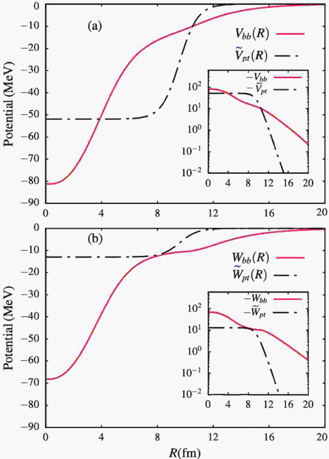
$ U_{bb}^{(N)}(R) $ and$ \widetilde{U}_{pt}^{(N)}(R) $ are plotted in Fig. 1. We observe in this figure that the potential$ U_{bb}^{(N)}(R) $ has a longer tail compared to the potential$ \widetilde{U}_{pt}^{(N)}(R) $ . This was expected, due to the long-tail extension of the$ ^{10}{\rm{Be}}+n $ ground-state wave function.
Figure 1. (color online) Plots of the real [panel (a)] and imaginary [panel (b)] parts of the potentials
$U_{bb}^{(N)}(R)$ and$\widetilde{U}_{pt}^{(N)}(R)$ , as functions of the centre of mass coordinate R.By comparing the two approaches, we should notice that, unlike
$ U^{(N)}_{bb}(R) $ , the potential$ \widetilde{U}_{pt}^{(N)}(R) $ is purely diagonal. The drawback is that, in this approach, the projectile is assumed to be a one-body system, such that it can resemble the case of a tightly bound two-body system, in which$ R_{ct}\simeq R_{nt}\simeq R $ . One can observe some pathology associated with this assumption in the breakup observables. In the absence of the continuum–continuum couplings, where$ U^{LJ}_{\alpha\alpha}(R) = U^{LL^\prime J}_{\alpha\alpha^\prime}(R) = 0 $ , the diagonal coupling matrix elements$ U_{\beta\beta}^{LJ} $ are reduced to the potential in the elastic scattering channel, and the first excited state channel. One can then anticipate a strong effect of the potentials$ \widetilde{U}_{pt}(R) $ and$ U_{bb}(R) $ in the absence of the continuum–continuum couplings. The importance of diagonal and off-diagonal continuum–continuum couplings is discussed in Ref. [24].In order to transform the projectile pure scattering wave functions into square-integrable bin wave functions, the relative core–nucleon momentum k is truncated at
$ k_{\rm{max}} $ , with the interval$ [0,k_{\rm{max}}] $ sliced into bins of width$ \Delta k_i = k_i-k_{i-1} $ . Next, one can follow the technique described in Ref. [38] for the bin wave functions,$ \varphi_\ell^j(k_i,r) $ :$ \varphi_\ell^j(k_i,r) = \sqrt{\frac{2}{\pi W_\alpha}}\int_{k_{i-1}}^{k_i}{\rm{g}}_\alpha(k) \phi_\ell^j(k,r){\rm d}k, $

(7) where
$ {\rm{g}}_\alpha(k) $ is some weight function, such that$W_{\alpha} = $ $ \int_{k_{i-1}}^{k_i}{\rm{g}}_{\alpha}(k){\rm d}k$ , with$ \phi_\ell^j(k,r) $ being pure scattering wave functions, normalized according to$ \phi_\ell^j(k,r)\stackrel{r\to\infty}\to \sin\left[kr-\frac{\ell\pi}{2}+\delta_{\ell j}(k)\right], $

(8) where
$ \delta_{\ell j}(k) $ are the associated nuclear phase shifts.After the coupling matrix elements which appear in Eq. (2) are obtained, the coupled differential equations (1) are solved by considering the usual boundary conditions in the asymptotic region, given by
$ {\cal{F}}_{\beta}^{LJ}(R) \stackrel{R\to\infty}\to \frac{\rm i}{2}\left[H_L^-(\rho)\delta_{\beta\beta^{\prime}}-H_L^+(\rho) S_{\beta\beta^{\prime}}^J(K_{\beta})\right], $

(9) where
$ H_L^{\pm}(\rho) $ ($ \rho = K_\beta R $ ) are the Coulomb Hankel functions,$ S_{\beta\beta^{\prime}}^J(K_{\beta}) $ being the scattering S-matrix, with$ K_\beta = \sqrt{\frac{2\mu_{pt}(E-\varepsilon_\beta)}{\hbar^2}} $ being theincident wave number. Various reaction observables can be derived from the S-matrix, as outlined for instance in Refs. [2, 38]. -
The parameters of the 10Be–n Woods–Saxon potential, which we use to obtain the different projectile energies and wave functions needed in the CDCC calculations, are the same as those considered in Refs. [36, 39]. These core–neutron parameters are:
$ V_0 = -59.5 $ MeV and$ V_{\rm{SO}} = 32.8 $ MeV fm2 for the depths of the central and spin–orbit (so) coupling terms, with$ R_0 = R_{\rm{SO}} = 2.699 $ fm and$ a_0 = a_{\rm{SO}} = 0.6 $ fm being the corresponding radii and diffuseness. As in Ref. [36], a partial-wave dependent depth$ V_{\ell>0} = -40.5 $ MeV was used to calculate the first excited bound state, the resonant and non-resonant continuum wave functions.For the numerical computation of the coupled differential equations, the different parameters used are summarized and described in Table 2. In this table, the interval
$ [0:\varepsilon_{\rm{max}}] $ was discretized into energy bins of widths$ \Delta\varepsilon = 0.5\,{\rm{MeV}} $ for the$ s- $ and$ p- $ states;$ \Delta\varepsilon = 1.0\,{\rm{MeV}} $ for the f- and d-states;$ \Delta\varepsilon = 1.5\,{\rm{MeV}} $ for${{g}}$ -states; and$ \Delta\varepsilon = 2.0\,{\rm{MeV}} $ for higher partial waves. Finer bins were considered for the resonant state. The numerical calculations were carried out using the Fresco code [40].Before we dive into the discussion of the results, let us first explain how the different breakup cross-sections were obtained. In the Coulomb breakup calculations, we switched off all the nuclear interactions in the coupling matrix elements
$ U_{\beta\beta^\prime}^{LL^\prime J} $ , such that the potential$ U_{pt} $ contains only the core–target Coulomb potential$ V_{ct}^{(C)} $ (since$ V_{nt}^{(C)} = 0 $ ). Then, we performed three different calculations: (i) when$ U^{(N)}_{bb} $ is added to the monopole Coulomb potential, as described in the previous subsection; (ii) when$ \widetilde{U}^{(N)}_{pt} $ is added to the monopole Coulomb potential; and (iii) when$ U^{(N)}_{bb} $ and$ \widetilde{U}^{(N)}_{pt} $ are removed, implying that only the monopole Coulomb potential is retained in the elastic scattering channel, referred as no-diagonal nuclear (“No DN”). The Coulomb breakup cross-sections obtained in (i) and (ii) contain the effect of nuclear absorption in the elastic channel. This will lead to a fusion cross-section, which does not contain the effect of the off-diagonal absorption. In the nuclear breakup calculations, we switched off all the Coulomb interactions in the couplings matrix elements$ U_{\beta\beta^\prime}^{LL^\prime J} $ , in which case the potential$ U_{pt} $ is reduced to its nuclear components$ U^{(N)}_{ct} = V_{ct}+{\rm{i}}W_{ct} $ , and$ U^{(N)}_{nt} = V_{nt}+{\rm{i}}W_{nt} $ . The resulting total fusion cross-section contains both complete and incomplete fusion components, due to the off-diagonal nuclear absorption. The total breakup calculations were performed by simultaneously including both Coulomb and nuclear components of the potential$ U_{pt} $ in the coupling matrix elements$ U_{\beta\beta^\prime}^{LL^\prime J} $ . Again, all three calculations outlined above were carried out. In all these calculations, the monopole Coulomb potential$ Z_pZ_te^2/R $ in the elastic scattering channel was retained. Although we are using an approximate procedure to obtain the Coulomb and nuclear breakup cross-sections, it is expected that the total breakup cross-section will approach its dominant component. This matter will be further analyzed in the following section. -
The angular distributions for the total, Coulomb and nuclear breakup cross-sections are shown in Fig. 2, as functions of the laboratory angle θ. They are calculated at the laboratory incident energy
$E_{\rm lab} = 140$ MeV. These results correspond to the three different calculations that we have outlined in Section II, and in the case where all the different couplings are included in the coupling matrix elements. We first observe, from panel (a) of Fig. 2, that a fair agreement is obtained between the total breakup cross-section and the experimental data obtained from Ref. [23]. We should mention that the measurements in this reference are inclusive, implying that the neutron was not measured in coincidence with the$ ^{10}{\rm{Be}} $ core nucleus after the breakup. In view of this, one can argue that the agreement with the calculations indicates the absorption of the valence neutron by the target through the potential$ W_{nt} $ , which represents the so-called stripping part of the cross-section.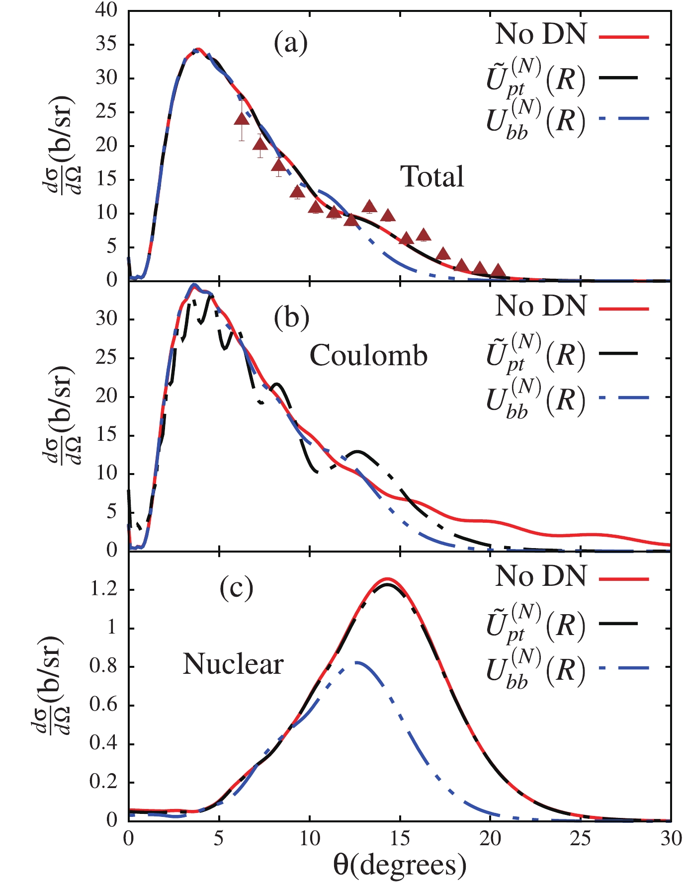
Figure 2. (color online) Angular distributions for the total (a), Coulomb (b) and nuclear (c) breakup cross-sections, obtained for the three different calculations outlined in the text, i.e. with the potentials
$\widetilde{U}^{(N)}_{pt}$ and$U_{bb}^{(N)}$ in the elastic scattering channel, and for the case labeled “No DN”, when there is no nuclear potential in the elastic scattering channel (meaning that$\widetilde{U}^{(N)}_{pt}=U_{bb}^{(N)}=0$ ). All the different couplings, including continuum–continuum couplings are taken into account. The experimental data in panel (a) were taken from Ref. [23].With regard to the relevance of the potentials
$ \widetilde{U}^{(N)}_{pt} $ and$ {U}^{(N)}_{bb} $ on the breakup cross-sections, we observe in panels (a) and (c) of Fig. 2 that the potential$ \widetilde{U}^{(N)}_{pt} $ plays a minor role in the total and nuclear breakups, as the corresponding curve and that corresponding to “No DN” are approximately similar. However, the relevance of the potential$ {U}^{(N)}_{bb} $ to the nuclear breakup cross-section in particular is clearly observed. Its verified effect is to suppress the total cross-section and to strongly suppress the nuclear cross-section. These results are highlighting the importance of the projectile ground-state wave function on the breakup cross-section, which is used to obtain the potential$ {U}^{(N)}_{bb} $ . The panel (b) displays a quite different trend in the Coulomb breakup, where a major effect of$ \widetilde{U}^{(N)}_{pt} $ is displayed, unlike in the total and nuclear breakup cases. One first observes that this potential suppresses the longer tail of the pure Coulomb breakup cross-section (“No DN”) at larger angles and also accounts for the oscillatory pattern in the cross-section that spans the whole angular range, despite its short-range nature. As in panel (a), the effect of the$ U^{(N)}_{bb} $ potential remains negligible at$ \theta \lesssim 10^\circ $ , but further suppresses the cross-section at larger angles. This observation is quite remarkable, since the potential$ \widetilde{U}^{(N)}_{pt} $ would be expected to have a minor effect on the Coulomb breakup cross-section compared to the nuclear breakup cross-section.The fact that the potential
$ \widetilde{U}^{(N)}_{pt} $ accounts for a negligible effect on the nuclear cross-section suggests that a negligible amount of flux from the elastic channel reaches the absorption region, unlike in the Coulomb breakup case. To understand the significance of the potential$ \widetilde{U}^{(N)}_{pt} $ in the Coulomb breakup, as well as its irrelevance to the nuclear breakup, we consider the case where the continuum–continuum couplings are removed from the coupling matrix elements. These couplings are known to enhance the irreversibility of the breakup process: once the projectile is dissociated, as the incident energy on the way back to bound-states cannot be recovered, the flux to bound-states is reduced (elastic scattering channel). The couplings are stronger in the nuclear than in the Coulomb breakup, so a larger amount of flux from the elastic scattering channel is expected to be removed. Primarily, it is this behavior that explains the different effect of the potential$ \widetilde{U}^{(N)}_{pt} $ on the Coulomb and nuclear breakup cross-sections in Fig. 2.The results shown in Fig. 3, for the three different calculations as in Fig. 2, are for the total, Coulomb and nuclear cross-sections, obtained when the continuum–continuum couplings are removed from the coupling matrix elements. These results are presented in order to understand how the negligible effect of the potential
$ \widetilde{U}^{(N)}_{pt} $ on the nuclear breakup cross-section in Fig. 2(c) could be associated with effects due to stronger continuum–continuum couplings in the nuclear breakup. It is interesting to observe that this figure now displays a major effect of the potential$ \widetilde{U}^{(N)}_{pt} $ on the total and nuclear cross-sections, which also spans the whole angular range. This indicates that the amount of flux from the elastic scattering, which would have been lost to continuum–continuum couplings, is absorbed through the imaginary part of$ \widetilde{U}^{(N)}_{pt} $ or$ U_{bb}^{(N)} $ . As already mentioned, in the absence of couplings among continuum states, the diagonal coupling matrix elements on the left side of Eq. (1) is reduced to its elastic scattering component, so that there is no interference between the potential$ \widetilde{U}^{(N)}_{pt} $ or$ U_{bb}^{(N)} $ and the diagonal coupling matrix elements$ U_{\alpha\alpha}^{LJ}(R) $ . These results also serve to further highlight the fact that the continuum–continuum couplings do indeed remove flux from the elastic scattering channel, which could have contributed to the fusion process (see Ref. [35], for example, for more related discussion).
Figure 3. (color online) Similar results as in Fig. 2, but in the case where the continuum–continuum couplings are removed from the coupling matrix elements in Eq. (2).
To better verify that the continuum–continuum couplings are stronger in the nuclear breakup than in the Coulomb breakup, we display in the panels of Fig. 4 the total, Coulomb and nuclear breakup cross-sections in the presence and absence of these couplings. From the results shown in this figure, it follows that when the continuum–continuum couplings are included in the coupling matrix elements, the Coulomb cross-section is substantially larger than the nuclear cross-section (see left panels). This was already anticipated, considering that the reaction under study is Coulomb-dominated. However, when these couplings are removed, the nuclear breakup cross-section becomes dominant at larger angles (
$ \theta\ge 10^\circ $ ), where it is approximately equal to the total breakup cross-section. From such a result, one can infer that the reduced nuclear cross-section (compared to its Coulomb counterpart in the left panels), is not only due to the short-range nature of nuclear forces, but also due to stronger continuum–continuum couplings in the nuclear breakup. Therefore, one may argue that the large target charge alone cannot justify the predominance of the Coulomb breakup over the nuclear breakup in a reaction involving a heavy target, such that the concept “Coulomb-dominated reaction” might be the subject of the prevailing reaction dynamics.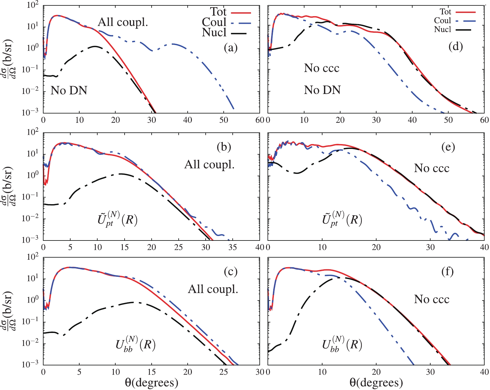
Figure 4. (color online) Comparison of the total, Coulomb and nuclear cross-sections when the continuum–continuum are included (left panels) and when they are excluded (right panels) from the coupling matrix elements. The results show all three calculations. See text for details.
Another aspect verified in Fig. 4 is that in the absence of any nuclear absorption in the elastic scattering channel (panel (a)), the total cross-section approaches its nuclear component at large angles, in spite of the fact that the Coulomb component is substantially dominant. One would naively expect the total cross-section to approach its dominant component. The rest of the panels clearly indicate that this “anomaly” can be attributed to (i) the absence of any nuclear absorption in the Coulomb breakup cross-section, and (ii) stronger continuum–continuum couplings in the nuclear breakup, which dictate the effect of these couplings in the total breakup. Again, one could argue that the trend that the total breakup should approach its dominant component does not come naturally. It rather depends on the prevailing reaction dynamics, at least as far as the reaction under study is concerned.
For a quantitative analysis of these results, we consider the integrated total, Coulomb and nuclear cross-sections for all three different kind of calculations in Table 3. In this table, in order to represent the factor by which the breakup cross-sections are reduced by the continuum–continuum couplings, we also estimate the respective ratios between the cross-sections without (nc) and with the couplings, given by
$\kappa_{{x}} = \sigma^{nc}_{{x}}/\sigma_{{x}}$ (${x}\equiv\rm total,~ Coul,~ nucl$ ). As shown, this factor is quite large for nuclear breakups compared with the Coulomb breakups. It is about 33 for “No DN” and 17 for both$ \widetilde{U}^{(N)}_{pt} $ and$ U^{(N)}_{bb} $ when considering the nuclear breakup; whereas for the Coulomb breakup it is only about 1.0. This further clarifies that the nuclear breakup cross-section is substantially affected by the continuum–continuum couplings compared to the Coulomb breakup cross-section. The effect of these couplings on the nuclear breakup is the main reason why the Coulomb cross-section is larger than its nuclear counterpart. For example, in the absence of any nuclear interaction in the elastic scattering channel, and when these couplings are not accounted for, the nuclear cross-section is substantially larger than the Coulomb cross-section. In this case, it is verified that the Coulomb breakup cross-section is about 64% of the corresponding nuclear counterpart ($\sigma_{\rm C}^{nc} = 0.64\sigma_{\rm nucl}^{nc}$ ), or that$\sigma_{\rm nucl}^{nc}$ has to be reduced by about 36% to reach$\sigma_{\rm C}^{nc}$ . This observation on the relevance of the continuum–continuum couplings serves to enforce our argument that, when considering reactions involving heavy targets, it is not only the large charge of the target that can justify the importance of the Coulomb breakup over the nuclear breakups.All couplings No couplings $\kappa_{\rm tot}$ 

$\kappa_{\rm C}$ 

$\kappa_{\rm nucl}$ 

$\sigma_{\rm tot}$ 

$\sigma_{\rm C}$ 

$\sigma_{\rm nucl}$ 

$\sigma^{nc}_{\rm tot}$ 

$\sigma^{nc}_{\rm C}$ 

$\sigma^{nc}_{\rm nucl}$ 

No DN 3928 6285 302 12780 6338 9893 3.25 1.00 32.76 $\widetilde{U}_{pt}^{(N)}$ 

3932 4454 298 8968 4911 4938 2.28 1.10 16.57 $U_{bb}^{(N)}$ 

3382 3684 150 6390 4002 2528 1.89 1.09 16.85 Table 3. Integrated total (
$\sigma_{\rm tot}$ ), Coulomb ($\sigma_{\rm C}$ ), and nuclear ($\sigma_{\rm nucl}$ ) breakup cross-sections (in mb), given in the presence (“All couplings”) and absence (“No couplings”) of the continuum–continuum couplings. The results are for all three different calculations described in the text, with$\kappa_{{x}}\equiv \sigma^{nc}_{{x}}/\sigma_{{x}}$ (x$\equiv\rm tot,~ C,~ nucl$ ).From Table 3, we can also extract the suppression factors for the x
$ = $ total, Coulomb and nuclear breakup cross-sections due to the potentials$ \widetilde{U}^{(N)}_{pt} $ and$ U^{(N)}_{bb} $ . For$ \widetilde{U}^{(N)}_{pt} $ , we define$\gamma_{{x}} = 1-\{\ \sigma_{{x}}[\widetilde{U}^{(N)}_{pt}]/\sigma_{{x}}({\rm{No\, DN}})\}$ ; and, for$ U^{(N)}_{bb} $ ,$\Sigma_{{x}} = 1-\{\ \sigma_{{x}}[{U}^{(N)}_{bb}]/\sigma_{{x}} ({\rm{No\, DN}})\}$ . While both$\gamma_{\rm tot}$ and$\gamma_{\rm nucl}$ are negligible when all the different couplings are included,$\gamma_{\rm Coul}\simeq 0.29$ (29%). When the continuum–continuum couplings are omitted, one obtains$\gamma_{\rm tot}\simeq 0.30$ ,$\gamma_{\rm nucl}\simeq 0.50$ , and$\gamma_{\rm Coul}\simeq 0.23$ , whereas$\Sigma_{\rm tot}\simeq 0.50$ ,$\Sigma_{\rm nucl}\simeq $ 0.74 and$\Sigma_{\rm Coul}\simeq 0.39$ .For the implication of the potentials
$ \widetilde{U}^{(N)}_{pt} $ and$ U^{(N)}_{bb} $ on the fusion cross-section, we analyze the total fusion cross-sections corresponding to the total, Coulomb and nuclear breakups. We should note that, in the Coulomb breakup, the fusion process is exclusively stimulated by the imaginary potential in the elastic scattering channel, namely$ \widetilde{W}^{(N)}_{pt} $ and$ W^{(N)}_{bb} $ . Since in this case$ \small{ {W_{\beta\beta^{\prime}}^{LL^{\prime}J}(R) = \langle{\cal{Y}}_{\beta}^{LJ} ({\boldsymbol{r}},\Omega_{\boldsymbol{R}})| W_{ct}+ W_{nt}| {\cal{Y}}_{\beta^{\prime}}^{L^{\prime}J}({\boldsymbol{r}}, \Omega_{\boldsymbol{R}})\rangle} = 0 } $ , the resulting fusion cross-section will have no dependence on the breakup channels. The partial L-distribution total fusion cross-sections are shown in Fig. 5. By looking at panel (a) for the$ \widetilde{W}^{(N)}_{pt} $ potential, one sees all three fusion cross-sections are similar at$ L\leqslant 60 $ with peaks at$ L\sim 60 - 70 $ . In the Coulomb breakup case, where$ W_{ct} = W_{nt} = 0 $ , the fusion cross-section rapidly drops to zero whereas fusion cross-sections corresponding to the total and nuclear breakups are extended to larger L. This extension certainly comes from the contribution of the off-diagonal$ W_{ct} $ and$ W_{nt} $ . This is confirmed in panel (b), where the fusion cross-section stimulated by$ W_{ct} $ and$ W_{nt} $ in the Coulomb breakup is now extended to larger values of L. To better understand these results, it could be interesting to consider incident energy below and around the Coulomb barrier. The results in panel (b) contain the effect of the long tail of the projectile ground-state wave function, which contributes to the fusion cross-section apart from the imaginary parts of the nuclear potentials. This effect is better identified in Fig. 6, where the fusion cross-section due to$ W_{bb}^{(N)} $ potential is larger at large angular momenta. One should be mindful of this in an actual analysis of fusion cross-sections (for more discussion, see Ref. [41]).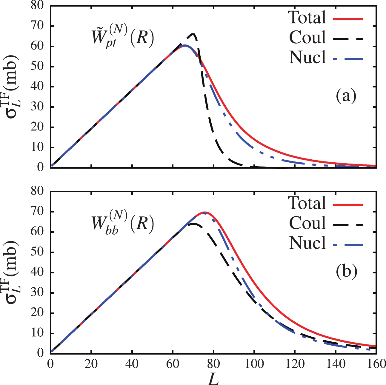
Figure 5. (color online) L-distribution total fusion cross-sections corresponding to total, Coulomb and nuclear breakups.
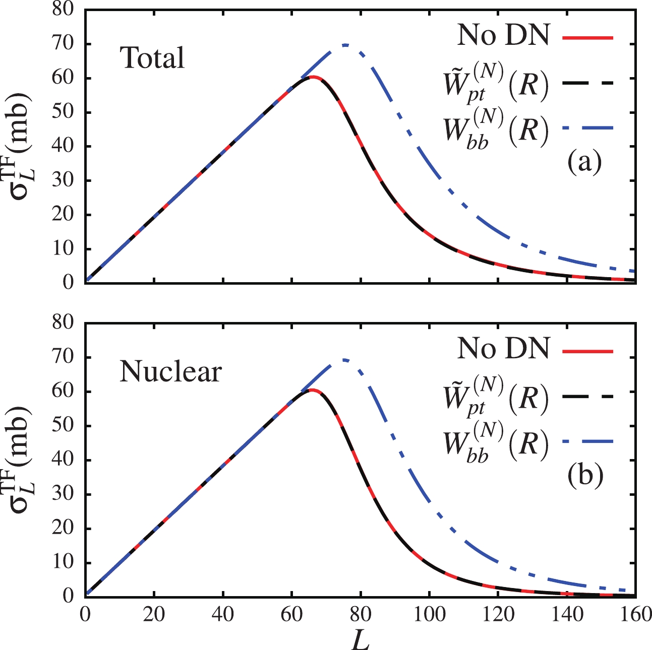
Figure 6. (color online) Comparison of L-distribution total fusion cross-sections corresponding to the three different calculations, in the case of total and nuclear breakups.
-
In order to clarify some aspects of the Coulomb and nuclear breakup dynamics, we have analyzed the breakup reaction of the weakly-bound one-neutron halo nucleus 11Be on the heavy target 208Pb. First, it was shown that the continuum–continuum couplings are much stronger in the nuclear breakup than in the Coulomb breakup, such that the strengths of these couplings in the continuum are dictated by the nuclear breakup when considering the total breakup. As a consequence, it was found that the diagonal monopole nuclear potential in the projectile–target c.m. has a negligible effect on the total and nuclear breakup cross-sections, while it suppresses the Coulomb breakup cross-section by about 29%, mainly at larger angles (absorption region). Such result is associated with the strong continuum–continuum couplings, which correspond to a substantial loss of flux from the diagonal channel to these couplings, implying that only a negligible portion of the flux reaches the absorption region in the total and nuclear breakups, as verified by the integrated results shown in Table 3.
When this diagonal nuclear potential is excluded from the calculations, the total cross-section approaches its nuclear component in the absorption region, in spite of the fact that the Coulomb breakup cross-section is largely important in this region. For the total breakup cross-section to approach its Coulomb component in the inner region, we show that the diagonal monopole nuclear potential (in the projectile–target c.m.) needs to be included in the calculations. It has the effect of absorbing the flux from the diagonal channel, which is not lost to the continuum–continuum couplings, considering the weakness in the Coulomb breakup in comparison to the nuclear breakup.
In the absence of the continuum–continuum couplings, there is no loss of flux, and the diagonal monopole nuclear potential is now found to suppress the total (by about 30%) and nuclear (by about 50%) breakup cross-sections, mainly in the absorption region (see also Table 3). When the monopole diagonal nuclear potential is obtained by folding the interactions between the fragments and the target, with the square of the ground-state projectile wave function, the total breakup cross-section is suppressed by about 50%, and the nuclear breakup cross-section by about 74%. By a quantitative analysis, it is verified that, when these couplings are excluded in the matrix elements, the Coulomb breakup cross-section is only about 64% of the corresponding nuclear breakup cross-section, in spite of the fact that this breakup reaction is recognized as a Coulomb-dominated reaction.
In summary, we observe the relevant role of the continuum–continuum couplings in the reaction studied so far. We conclude that the condition for the total breakup to approach its dominant component in the absorption region is determined by these continuum–continuum couplings. Moreover, it is a large charge, together with continuum–continuum couplings that justify the concept “Coulomb-dominated reaction”, and not a large target charge alone. The present results are expected to provide a further step in the quest to understand reaction dynamics associated with the breakup of loosely-bound systems in reaction to heavy nuclear targets. Also, such results may be useful in probing the origin of complete fusion suppression.
Coulomb and nuclear interactions in the dynamics of weakly-bound neutron-halo breakup on heavy target
- Received Date: 2021-07-21
- Available Online: 2022-01-15
Abstract: Within our aim to clarify some aspects of the breakup dynamics of loosely-bound neutron-halo projectiles on a heavy target, we apply the continuum discretized coupled-channel formalism to investigate the beryllium 11Be breakup on a lead 208Pb target at


 DownLoad: