


 Abstract
 HTML
HTML Reference
 Related
 PDF
PDF


-
The modified theories of gravity were motivated by the theoretical complications at the high and low curvature regions of Einstein's theory of general relativity. Existing theories in literature largely utilize one of two approaches. The first approach introduces modifications to the classical theory of gravity, by incorporating either further corrections to the curvature sector or additional degrees of freedom to the original Einstein-Hilbert action. For example, the former consists of the Gauss-Bonnet and Lovelock [1],
$ f(R) $ [2],$ f(T) $ [3], and$ f(R, T) $ [4] theories, while the latter includes the scalar-tensor [5] and scalar-tensor-vector [6, 7] theories, along with others. The second approach involves deriving the theory as an effective action from a more fundamental framework, such as string theory. A notable example of such a theory is Hořava-Lifshitz gravity [8-10]. The scalar-tensor theories are characterized by a scalar field coupled to the curvature sector. The crucial aspect of the theory is that it must evade a variety of no-hair theorems, which potentially rule out any regular hair. The latter is most relevant in asymptotically flat spacetimes [11, 12]. Known examples of the successful "implant" of a scalar field include the inclusion of the nonlinear electromagnetic field [13], derivative coupling [14], or the coupling to the higher curvature invariants. The extended scalar-tensor-Gauss-Bonnet gravity (STGB) belongs to the last scenario, which also can be viewed, from the Einstein frame, as an effective action of string theory [15]. Moreover, the theory accommodates spontaneous scalarization [16-20]. Specifically, the presence of the Gauss-Bonnet term acts as a catalyst for the scalar hair to emerge [21]. The resultant scalarization was shown to be regular and thermodynamically favorable with respect to its counterparts in general relativity. Interestingly, the resultant hairy black hole metrics in STGB gravity often feature discrete families of solutions, which differ from each other by the number of nodes in the scalar hair.More recently, the STGB theory was further generalized to consider Born-Infeld nonlinear electromagnetic fields [22, 23], and a class of analytic black hole solutions was obtained [24]. Characterized by a nonzero magnetic charge q, many new properties were observed for the derived metrics. They describe black holes with different structures featuring two bifurcation points, governed by the specific model parameters q and ADM mass m. Specifically, the resultant black holes behave mostly like the Schwarzschild metric, for
$ m\ge 0 $ and$ q\ge 0 $ . For$ m>0 $ and$ q<0 $ , the solutions are reminiscent of that of the Reissner-Nordström solution, while for$ m = 0 $ , a purely magnetic black hole is obtained.From an empirical point of view, such hairy black holes may lead to distinct observable implications, such as the strongly lensing effect of electrodynamic signals, including chaotic lensing [25] and cuspy shadows [26, 27]. Additionally, gravitational waves, quasinormal modes [28, 29], and echoes [30] are also important topics. The distinctive complex frequencies of the characteristic dissipative oscillations of black hole quasinormal modes are understood to carry intrinsic information about the black hole spacetime. Furthermore, the black hole echoes are expected to be strongly associated with the spacetime curvature of the strong-field region in the vicinity of the horizon. However, it has been pointed out the possible perturbations to spacetime configurations due to external fields, referred to as "dirty" black holes, might substantially affect the quasinormal spectra [31, 32] as well as the echo patterns [33]. The former has been recently further explored in terms of the stability of the quasinormal modes [31, 34] using hyperboloidal coordinates [35]. Therefore, one might expect to detect the presence of the scalar hair in the underlying theories from such pertinent distinctive features. Subsequently, this study was motivated to investigate the scalar and Dirac quasinormal modes in the extended STGB theory.
The remainder of the paper is organized as follows. In Sec. II, we briefly review the analytic black hole solutions that are explored in this study. We show that different metrics can be classified in terms of their respective horizon structures, from which two specific cases are further explored. In Sec. III, the master equations for the scalar and Dirac perturbations are derived. The numerical calculations are presented in Sec. IV, where we employ both the WKB approximation and finite difference method. The last section is devoted to further discussions and concluding remarks.
-
Recently, Cañate and Bergliaffa proposed the following novel analytic magnetic black hole solution in the extended STGB theory [24]:
$ \begin{equation} {\rm d}s^2 = -f(r){\rm d}t^2+\frac{{\rm d}r^2}{f(r)}+r^2\left({\rm d}\theta^2+\sin^2\theta {\rm d}\varphi^2\right), \end{equation} $

(1) where
$ \begin{equation} f(r) = 1-\frac{2m}{r}-\frac{q^3}{r^3} . \end{equation} $

(2) Based on the properties of horizons which are governed by
$ f(r) = 0 $ , in this study, we elaborate on two distinct cases.For the first case (Case 1), there is only one positive real root, giving the event horizon
$ r_p $ , and two complex roots, so that$ \begin{equation} f_1(r) = \left(1-\frac{r_p}{r}\right)\left(1+\frac{A}{r}+\frac{B}{r^2}\right) , \end{equation} $

(3) where
$ A $ and$ B $ are two real parameters that satisfy$ A^2 < 4B $ . Moreover, by comparing Eq. (3) to the metric Eq. (1), we have$ \begin{eqnarray} A = \frac{q^3}{r_p^2},\; \; \; \; \; B = \frac{q^3}{r_p},\; \; \; \; \; m = \frac{r_p}{2}-\frac{q^3}{2r_p^2} . \end{eqnarray} $

(4) For the second case (Case 2), there are two positive real roots, giving the event horizon
$ r_p $ and inner horizon$ r_i\equiv Cr_p $ , and one negative real root$ r = -D <0 $ , and we have$ \begin{equation} f_2(r) = \left(1-\frac{r_p}{r}\right)\left(1-C\frac{r_p}{r}\right)\left(1+\frac{D}{r}\right) , \end{equation} $

(5) where
$ 0\leqslant C\leqslant 1 $ , which becomes an extreme black hole when$ C = 1 $ , and$ \begin{aligned}[b] D= &\frac{Cr_p}{1+C},\;\; \; m = \frac{(1+C+C^2)r_p}{2(1+C)}, \;\;\; q= -\frac{C^{2/3}r_p}{(1+C)^{1/3}}. \end{aligned} $

(6) It seems plausible to consider a third case where one has one positive real root as the event horizon
$ r_p $ as well as two negative roots, namely,$ r = -E<0 $ and$ r = -F<0 $ . However, it can be shown that this is not a physically relevant scenario, as the above horizon structure implies that$ \begin{equation} f_3(r) = \left(1-\frac{r_p}{r}\right)\left(1+E\frac{r_p}{r}\right)\left(1+\frac{F}{r}\right), \end{equation} $

(7) where
$ \begin{aligned}[b] F = &\frac{Er_p}{E-1},\; \;\; \; m = \frac{(E^2-E+1)r_p}{2(1-E)}, \;\;\;\; q = \frac{E^{2/3}r_p}{(E-1)^{1/3}} . \end{aligned} $

(8) As the mass of the black hole is positive definite, the relation between m and E implies that
$ 0<E<1 $ , which in turn means$ F<0 $ ; this contradicts our assumption. By employing similar arguments, one can also show that the solution of three positive roots must be excluded. In the following sections, we explore the quasinormal perturbations in the background metrics determined by Case 1 and Case 2. -
In this section, we derive the relevant master equations for the scalar and Dirac perturbations. In curved spacetime, the equation of motion for massless scalar perturbations satisfies
$ \begin{eqnarray} \partial_\mu\left(\sqrt{-g}g^{\mu\nu}\partial_\nu\Phi\right) = 0 . \end{eqnarray} $

(9) We note that here the field Φ is not the scalar degree of freedom of the STGB theory, but an external scalar field that is minimally coupled to the background metric, which is introduced to probe the stability of the metric. To proceed, one further assumes that
$ \Phi = {\rm e}^{-{\rm i}\omega t}Y(\theta,\varphi)\phi(r) $ , where$ Y(\theta,\varphi) $ are the spherical harmonics. By separating the variables, the resulting radial component reads$ \begin{eqnarray} \frac{{\rm d}^2\phi}{{\rm d}r_*^2}+(\omega^2-V(r))\phi = 0 , \end{eqnarray} $

(10) where
$ V(r) = \frac{f(r)}{r^2}\left(L^2+L+rf'(r)\right) , $

(11) and
$ r_* = \int {\rm d}r/f(r) $ is the tortoise coordinate.Then, the Dirac equation in curved spacetime is
$ \begin{eqnarray} \gamma^ae^\mu_a\left(\partial_\mu+\Gamma_\mu\right)\Psi = 0, \end{eqnarray} $

(12) where
$ \begin{aligned}[b] \Gamma_\mu= &\frac{1}{8}\left[\gamma^a,\gamma^b\right]e^\nu_ae^b_\nu, \\ e^a_\mu = &\text{diag}\left(\sqrt{f},1/\sqrt{f},r,r\sin\theta\right), \end{aligned} $

(13) and
$ \gamma^a $ is the gamma matrix in flat spacetime. To proceed, one introduces the ansatz proposed by Cho [36]$ \Psi = {\rm e}^{-{\rm i}\omega t}\frac{f(r)^{-1/4}}{r}\left(\begin{array}{cc} {\rm i}G^{\pm}(r)\phi^{\pm}_{jm}(\theta,\varphi) \\ F^{\pm}(r)\phi^{\mp}_{jm}(\theta,\varphi) \end{array}\right) $

(14) where one assumes the form of a stationary state and focuses on the definite angular quantum number, namely,
$ \begin{aligned}[b] \phi^+_{jm} =& \left(\begin{array}{cc} \sqrt{\dfrac{L+1/2+m}{2L+1}}Y^{m-1/2}_L \\ \sqrt{\dfrac{L+1/2-m}{2L+1}}Y^{m+1/2}_L \end{array}\right)\; \; \; \text{for}\; j = L+\frac{1}{2}, \\ \phi^-_{jm} = &\left(\begin{array}{cc} \sqrt{\dfrac{L+1/2-m}{2L+1}}Y^{m-1/2}_L \\ -\sqrt{\dfrac{L+1/2+m}{2L+1}}Y^{m+1/2}_L \\ \end{array}\right)\; \; \; \text{for}\; j = L-\frac{1}{2} \\ \end{aligned} $

(15) which are eigenfunctions of the total angular momentum
$ {J}^2 $ .The resultant radial equation reads
$ \begin{aligned}[b]& \frac{\rm d}{{\rm d}r_*} \left(\begin{array}{cc} F^\pm\\ G^\pm\\ \end{array}\right) -\sqrt{f(r)} \left(\begin{array}{cc} \kappa_\pm/r & 0 \\ 0 & -\kappa_\pm/r\\ \end{array}\right) \left(\begin{array}{cc} F^\pm\\ G^\pm\\ \end{array}\right) \\ = &\left(\begin{array}{cc} 0 & -\omega \\ \omega & 0\\ \end{array}\right) \left(\begin{array}{cc} F^\pm\\ G^\pm\\ \end{array}\right) , \end{aligned} $

(16) where
$ \begin{eqnarray} \kappa_{(\pm)} = \left\{\begin{array}{cc} -(j+1/2),&j = L+1/2\\ j+1/2,&j = L-1/2\\ \end{array}\right. . \end{eqnarray} $

(17) From Eq. (16), one derives the decoupled equations for
$ F^\pm $ and$ G^\pm $ $ \begin{aligned}[b]& \frac{{\rm d}^2F^\pm}{{\rm d}r_*^2}+\left(\omega^2-\bar{V}_\pm\right)F^\pm = 0 , \\& \frac{{\rm d}^2G^\pm}{{\rm d}r_*^2}+\left(\omega^2-\hat{V}_\pm\right)G^\pm = 0 , \end{aligned} $

(18) where
$ \begin{aligned}[b] \bar{V}_\pm = &\frac{{\rm d}W_\pm}{{\rm d}r_*}+W_\pm^2, \quad \hat{V}_\pm = -\frac{{\rm d}W_\pm}{{\rm d}r_*}+W_\pm^2, \\ W_\pm = &\frac{\kappa_\pm}{r}\sqrt{f(r)}. \end{aligned} $

(19) As the two effective potentials with plus and minus signs are related to each other through the Darboux transformation [36, 37], in what follows, we omit the superscript and present the result in terms of the amplitude
$ F\equiv F^{+} $ .The quasinormal modes can be evaluated by solving these master equations with physically appropriate boundary conditions. Specifically, the wave function must be outgoing at infinity and ingoing at the event horizon. By taking into account that the effective potentials V,
$ \hat{V} $ , and$ \bar{V} $ vanish at infinity and the event horizon, the asymptotic forms of the wave functions are$ \propto {\rm e}^{{\rm i}\omega r_*} $ at infinity and$ \propto {\rm e}^{-{\rm i}\omega r_*} $ at the horizon. -
In this study, we solve for the quasinormal frequencies by employing two methods, the WKB approximation [38-40] and the finite difference method [41].
The WKB approximation is a semi-analytic approach that is reminiscent of solving for the scattering resonances in a one-dimensional quantum mechanical scattering problem near the peak of a potential barrier. According to this method, the eigenvalues of the complex frequencies are given by
$ \begin{eqnarray} \left.\frac{{\rm i}\left(\omega^2-V(r)\right)}{\sqrt{-2V''}}\right|_{r = x_0} = n+\frac{1}{2}+\sum_{j = 2}\Lambda_j , \end{eqnarray} $

(20) where
$ x_0 $ is the coordinate of the maximum of the potential V, and$ \Lambda_j $ are the correction terms owing to the WKB method. The resultant quasinormal frequencies evaluated using the third and sixth order approaches are given in Tables 1-6.L q $\omega \text{ (sixth-order)}$ 

$\omega \text{ (third-order)}$ 

0 $0.1$ 

$0.2210 - 0.2019{\rm i}$ 

$0.2093 - 0.2308{\rm i}$ 

$0.2$ 

$0.2214 - 0.2040{\rm i}$ 

$0.2097 - 0.2334{\rm i}$ 

$0.3$ 

$0.2224 - 0.2105{\rm i}$ 

$0.2102 - 0.2408{\rm i}$ 

1 $0.1$ 

$0.5861 - 0.1958{\rm i}$ 

$0.5825 - 0.1963{\rm i}$ 

$0.2$ 

$0.5883 - 0.1976{\rm i}$ 

$0.5847 - 0.1981{\rm i}$ 

$0.3$ 

$0.5941 - 0.2025{\rm i}$ 

$0.5903 - 0.2032{\rm i}$ 

2 $0.1$ 

$0.9678 - 0.1938{\rm i}$ 

$0.9669 - 0.1939{\rm i}$ 

$0.2$ 

$0.9715 - 0.1956{\rm i}$ 

$0.9706 - 0.1957{\rm i}$ 

$0.3$ 

$0.9814 - 0.2004{\rm i}$ 

$0.9806 - 0.2006{\rm i}$ 

3 $0.1$ 

$1.3515 - 0.1933{\rm i}$ 

$1.3511 - 0.1933{\rm i}$ 

$0.2$ 

$1.3567 - 0.1950{\rm i}$ 

$1.3564 - 0.1950{\rm i}$ 

$0.3$ 

$1.3707 - 0.1999{\rm i}$ 

$1.3704 - 0.1999{\rm i}$ 

Table 1. The lowest lying scalar quasinormal modes obtained using the WKB approximation for Case 1 with
$r_p=1$ .L C $\omega \text{ (sixth-order)}$ 

$\omega \text{ (third-order)}$ 

0 $0$ 

$0.2209 - 0.2016{\rm i}$ 

$0.2093 - 0.2304{\rm i}$ 

$0.25$ 

$0.2170 - 0.1899{\rm i}$ 

$0.2041 - 0.2120{\rm i}$ 

$0.5$ 

$0.2139 - 0.1420{\rm i}$ 

$0.1795 - 0.1764{\rm i}$ 

$0.75$ 

$0.1780 - 0.1178{\rm i}$ 

$0.1523 - 0.1515{\rm i}$ 

1 $0$ 

$0.5858 - 0.1955{\rm i}$ 

$0.5822 - 0.1960{\rm i}$ 

$0.25$ 

$0.5701 - 0.1830{\rm i}$ 

$0.5666 - 0.1831{\rm i}$ 

$0.5$ 

$0.5319 - 0.1565{\rm i}$ 

$0.5276 - 0.1563{\rm i}$ 

$0.75$ 

$0.4793 - 0.1306{\rm i}$ 

$0.4751 - 0.1306{\rm i}$ 

2 $0$ 

$0.9673 - 0.1935{\rm i}$ 

$0.9664 - 0.1936{\rm i}$ 

$0.25$ 

$0.9407 - 0.1812{\rm i}$ 

$0.9398 - 0.1812{\rm i}$ 

$0.5$ 

$0.8771 - 0.1556{\rm i}$ 

$0.8761 - 0.1555{\rm i}$ 

$0.75$ 

$0.7926 - 0.1301{\rm i}$ 

$0.7916 - 0.1301{\rm i}$ 

3 $0$ 

$1.3507 - 0.1930{\rm i}$ 

$1.3504 - 0.1930{\rm i}$ 

$0.25$ 

$1.3133 - 0.1808{\rm i}$ 

$1.3130 - 0.1808{\rm i}$ 

$0.5$ 

$1.2246 - 0.1553{\rm i}$ 

$1.2242 - 0.1553{\rm i}$ 

$0.75$ 

$1.1074 - 0.1230{\rm i}$ 

$1.1070 - 0.1300{\rm i}$ 

Table 2. The lowest lying scalar quasinormal modes obtained using the WKB approximation for non-extreme black holes in Case 2 with
$r_p=1$ .L $\omega \text{ (sixth-order)}$ 

$\omega \text{ (third-order)}$ 

0 $0.1557 - 0.1037{\rm i}$ 

$0.1332 - 0.1334{\rm i}$ 

1 $0.4242 - 0.1129{\rm i}$ 

$0.4205 - 0.1129{\rm i}$ 

2 $0.7027 - 0.1123{\rm i}$ 

$0.7018 - 0.1123{\rm i}$ 

3 $0.9822 - 0.1122{\rm i}$ 

$0.9819 - 0.1121{\rm i}$ 

Table 3. The lowest lying scalar quasinormal modes obtained using the WKB approximation for extreme black holes in Case 2 with
$r_p=1$ .L q $\omega \text{ (sixth-order)}$ 

$\omega \text{ (third-order)}$ 

1 $0.01$ 

$0.3662 - 0.1941{\rm i}$ 

$0.3631 - 0.1945{\rm i}$ 

$0.3$ 

$0.3708 - 0.2014{\rm i}$ 

$0.3682 - 0.2016{\rm i}$ 

$0.6$ 

$0.3999 - 0.2535{\rm i}$ 

$0.3977 - 0.2551{\rm i}$ 

2 $0.01$ 

$0.7601 - 0.1928{\rm i}$ 

$0.7594 - 0.1929{\rm i}$ 

$0.3$ 

$0.7710 - 0.1998{\rm i}$ 

$0.7705 - 0.1999{\rm i}$ 

$0.6$ 

$0.8436 - 0.2518{\rm i}$ 

$0.8434 - 0.2521{\rm i}$ 

3 $0.01$ 

$1.1482 - 0.1926{\rm i}$ 

$1.1479 - 0.1926{\rm i}$ 

$0.3$ 

$1.1651 - 0.1995{\rm i}$ 

$1.1649 - 0.1995{\rm i}$ 

$0.6$ 

$1.2788 - 0.2514{\rm i}$ 

$1.2787 - 0.2515{\rm i}$ 

Table 4. The lowest lying Dirac quasinormal modes obtained using the WKB approximation for Case 1 with
$r_p=1$ .L C $\omega \text{ (sixth-order)}$ 

$\omega \text{ (third-order)}$ 

1 $0$ 

$0.3662 - 0.1941{\rm i}$ 

$0.3631 - 0.1945{\rm i}$ 

$0.25$ 

$0.3571 - 0.1809{\rm i}$ 

$0.3531 - 0.1818{\rm i}$ 

$0.5$ 

$0.3327 - 0.1529{\rm i}$ 

$0.3277 - 0.1555{\rm i}$ 

$0.75$ 

$0.2962 - 0.1278{\rm i}$ 

$0.2933 - 0.1306{\rm i}$ 

2 $0$ 

$0.7601 - 0.1928{\rm i}$ 

$0.7594 - 0.1929{\rm i}$ 

$0.25$ 

$0.7394 - 0.1805{\rm i}$ 

$0.7386 - 0.1806{\rm i}$ 

$0.5$ 

$0.6896 - 0.1547{\rm i}$ 

$0.6884 - 0.1549{\rm i}$ 

$0.75$ 

$0.6227 - 0.1292{\rm i}$ 

$0.6214 - 0.1295{\rm i}$ 

3 $0$ 

$1.1482 - 0.1926{\rm i}$ 

$1.1479 - 0.1926{\rm i}$ 

$0.25$ 

$1.1165 - 0.1804{\rm i}$ 

$1.1162 - 0.1804{\rm i}$ 

$0.5$ 

$1.0412 - 0.1549{\rm i}$ 

$1.0407 - 0.1549{\rm i}$ 

$0.75$ 

$0.9414 - 0.1296{\rm i}$ 

$0.9409 - 0.1296{\rm i}$ 

Table 5. The lowest lying Dirac quasinormal modes obtained using the WKB approximation for non-extreme black holes in Case 2 with
$ r_p=1.$ L $\omega \text{ (sixth-order)}$ 

$\omega \text{ (third-order)}$ 

1 $0.2609 - 0.1111{\rm i}$ 

$0.2590 - 0.1134{\rm i}$ 

2 $0.5518 - 0.1116{\rm i}$ 

$0.5506 - 0.1119{\rm i}$ 

3 $0.8349 - 0.1118{\rm i}$ 

$0.8344 - 0.1119{\rm i}$ 

Table 6. The lowest lying Dirac quasinormal modes obtained using the WKB approximation for extreme black holes in Case 2 with
$r_p=1$ .From the results presented in Tables 1-6, we find that the obtained quasinormal frequencies are strongly dependent on the black hole parameters. In other words, if such complex frequencies can be extracted from the measured dissipative oscillations, they can be utilized to identify the underlying spacetime metric. For Case 1, when the parameter q increases, the absolute values of the real part
$ |\omega_{\rm R}| $ and imaginary part$ |\omega_{\rm I}| $ of the frequency both increase. This indicates that, when compared with Schwarzschild black holes, the ESTGB black holes possess smaller oscillation periods with faster amplitude decay. However, for Case 2,$ |\omega_{\rm R}| $ and$ |\omega_{\rm I}| $ both decrease as the parameter C increases. In turn, this implies that the ESTGB black holes possess larger oscillation periods and the dissipations occur at a lower rate when compared with the Schwarzschild case with two horizons.Furthermore, it is of interest to investigate the scalar and Dirac perturbations in a purely magnetic black hole. Such a spacetime configuration corresponds to a particular choice of metric so that the mass parameter of the resulting black hole vanishes. To investigate such a scenario, we choose to tune one of the metric parameters while keeping the others constant, so that the mass of the black hole approaches that of a purely magnetic black hole. The results of the calculations for Case 1, where the horizon is chosen as
$ r_p = 1 $ , are presented in Tables 7 and 8 for the scalar and Dirac perturbations, respectively, for various angular momentum states. For this specific case, the mass parameter$ m\to 0 $ from above as$ q\to 1 $ from below. For scalar perturbations, it is observed that the magnitudes of both the real and imaginary parts of the quasinormal frequencies increase when the metric becomes that of a purely magnetic black hole. For Dirac perturbations, similar behavior is observed as one approaches the limit of the purely magnetic metric. Moreover, for both cases, it is found that the quasinormal frequency changes smoothly as the metric approaches this limit.L q $\omega\text{ (sixth-order)}$ 

$\omega\text{ (third-order)}$ 

1 $0.8$ 

$0.7021 - 0.3751{\rm i}$ 

$0.6845 - 0.3481{\rm i}$ 

$0.9$ 

$0.7499 - 0.4557{\rm i}$ 

$0.6997 - 0.4221{\rm i}$ 

$0.95$ 

$0.7874 - 0.4887{\rm i}$ 

$0.7037 - 0.4700{\rm i}$ 

$1$ 

$0.8348 - 0.5124{\rm i}$ 

$0.7054 - 0.5275{\rm i}$ 

2 $0.8$ 

$1.2108 - 0.3423{\rm i}$ 

$1.2047 - 0.3431{\rm i}$ 

$0.9$ 

$1.2981 - 0.4128{\rm i}$ 

$1.2872 - 0.4118{\rm i}$ 

$0.95$ 

$1.3452 - 0.4566{\rm i}$ 

$1.3313 - 0.4531{\rm i}$ 

$1$ 

$1.3935 - 0.5075{\rm i}$ 

$1.3764 - 0.4992{\rm i}$ 

3 $0.8$ 

$1.6997 - 0.3411{\rm i}$ 

$1.6979 - 0.3416{\rm i}$ 

$0.9$ 

$1.8293 - 0.4093{\rm i}$ 

$1.8257 - 0.4101{\rm i}$ 

$0.95$ 

$1.9016 - 0.4503{\rm i}$ 

$1.8965 - 0.4513{\rm i}$ 

$1$ 

$1.9786 - 0.4963{\rm i}$ 

$1.9715 - 0.4974{\rm i}$ 

Table 7. The lowest lying scalar quasinormal modes as the mass of the black hole approaches that of a purely magnetic one for Case 1 with
$r_p=1$ . Here, the mass parameter$m\to 0^+$ from above as$q\to 1^-$ from below. The calculations were obtained using the WKB approximation.L q $\omega\text{ (sixth-order)}$ 

$\omega\text{ (third-order)}$ 

1 $0.8$ 

$0.4345 - 0.3401{\rm i}$ 

$0.4262 - 0.3467{\rm i}$ 

$0.9$ 

$0.4536 - 0.4055{\rm i}$ 

$0.4383 - 0.4181{\rm i}$ 

$0.95$ 

$0.4629 - 0.4444{\rm i}$ 

$0.4429 - 0.4618{\rm i}$ 

$1$ 

$0.4717 - 0.4875{\rm i}$ 

$0.4463 - 0.5113{\rm i}$ 

2 $0.8$ 

$0.9443 - 0.3409{\rm i}$ 

$0.9433 - 0.3414{\rm i}$ 

$0.9$ 

$1.0096 - 0.4089{\rm i}$ 

$1.0074 - 0.4099{\rm i}$ 

$0.95$ 

$1.0454 - 0.4498{\rm i}$ 

$1.0423 - 0.4511{\rm i}$ 

$1$ 

$1.0831 - 0.4956{\rm i}$ 

$1.0788 - 0.4973{\rm i}$ 

3 $0.8$ 

$1.4408 - 0.3403{\rm i}$ 

$1.4405 - 0.3405{\rm i}$ 

$0.9$ 

$1.5484 - 0.4083{\rm i}$ 

$1.5477 - 0.4087{\rm i}$ 

$0.95$ 

$1.6083 - 0.4491{\rm i}$ 

$1.6073 - 0.4496{\rm i}$ 

$1$ 

$1.6718 - 0.4948{\rm i}$ 

$1.6705 - 0.4954{\rm i}$ 

Table 8. The lowest lying Dirac quasinormal modes as the mass of the black hole approaches that of a purely magnetic one for Case 1 with
$r_p=1$ . Here, the mass parameter$m\to 0^+$ from above as$q\to 1^-$ from below. The calculations were obtained using the WKB approximation.Now, we proceed to evaluate the time-domain evolution of the scalar and Dirac perturbations using the finite difference method [41]. The method is implemented by introducing the following light-cone coordinate transformation
$ u = t-r_* $ and$ v = t+r_* $ . Subsequently, the spatial boundary of the problem is properly transfered in the new coordinate system, and the perturbation equation of the wavefunction R with potential V becomes$ \begin{eqnarray} 4\frac{\partial^2R}{\partial u\partial v}+V(r)R = 0 . \end{eqnarray} $

(21) One may then discretize the above equation to obtain
$ \begin{aligned}[b] R(u+\Delta,v+\Delta) = &R(u,v+\Delta)+R(u+\Delta,v)-R(u,v) \\ &-\frac{\Delta^2}{4}V(r)R(u,v)+{\cal O}(\epsilon^4) . \end{aligned} $

(22) The initial and boundary conditions are given by
$ \begin{eqnarray} R(u = u_0,v) = {\rm e}^{-\frac{(v-v_c)^2}{2\sigma^2}},\; \; \quad R(u,v = v_0) = 0 , \end{eqnarray} $

(23) where
$ u_0 $ ,$ v_0 $ , σ,$ v_c $ are chosen for the specific form of the initial Gaussion waveform and the boundary. We present the resulting temporal evolutions of the perturbations in Figs. 1-5.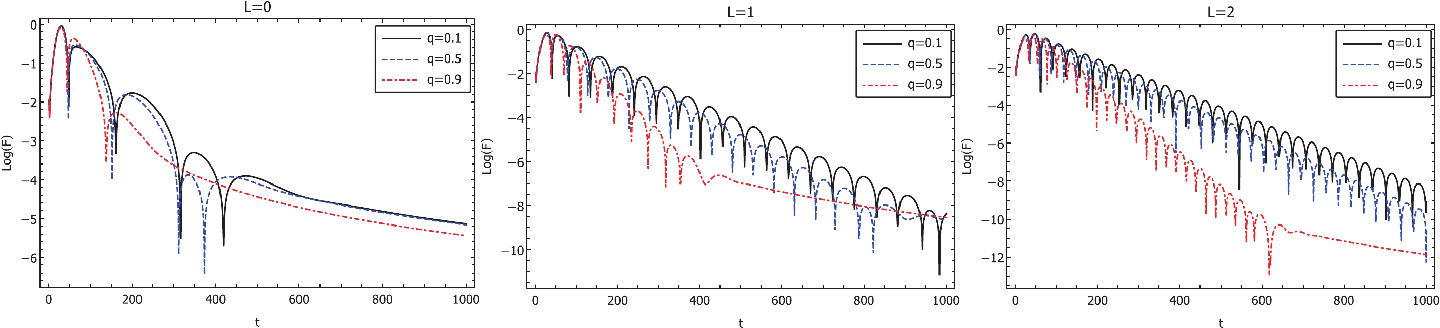
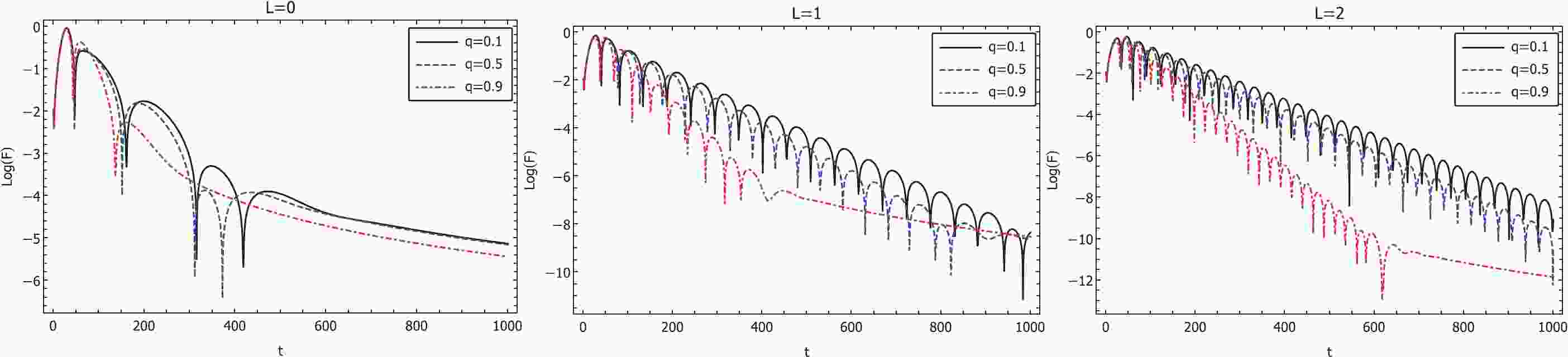
Figure 1. (color online) The calculated temporal evolution of the scalar perturbations for Case 1 with
$ r_p = 1 $ .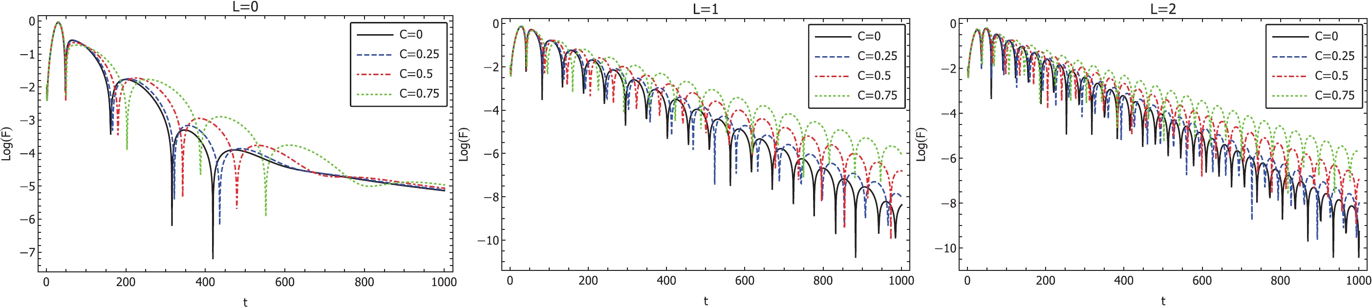
Figure 2. (color online) The calculated temporal evolution of the scalar perturbations for non-extreme black holes of case 2 with
$ r_p = 1 $ .
Figure 3. (color online) The calculated temporal evolution of the scalar (left) and Dirac (right) perturbations for extreme black holes in Case 2 with
$ r_p = 1 $ .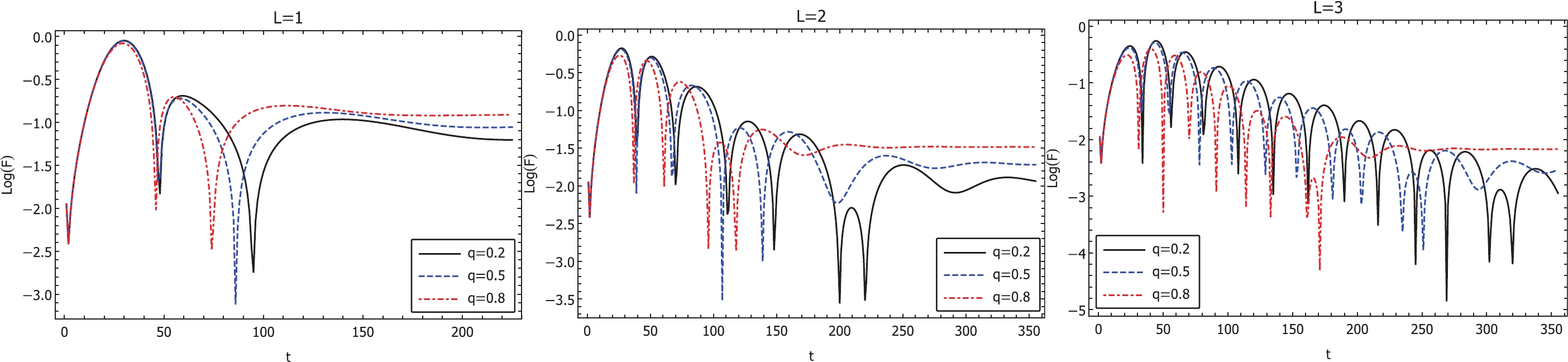
Figure 4. (color online) The calculated temporal evolution of the Dirac perturbations for Case 1 with
$ r_p = 1 $ .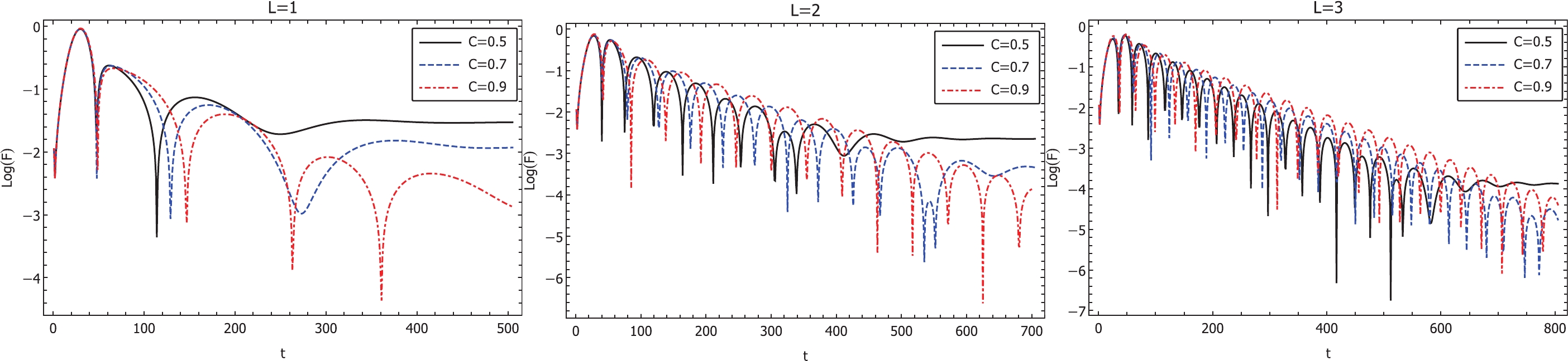
Figure 5. (color online) The calculated temporal evolution of the Dirac perturbations for non-extreme black holes in Case 2 with
$ r_p = 1 $ .From the calculated temporal oscillations displayed in Figs. 1-5, one observes that the results from the finite difference method support the results obtained using the WKB approximation. The above conclusion can be drawn by analyzing the oscillation periods and the rates of amplitude dissipation, as well as their dependence on the black hole parameters. Moreover, at significantly later times for scalar perturbations, late-time tails can be observed. We understand that the latter is due to the effective potential decaying fast enough at spatial infinity, leading to backscattering of the initial waveform [42, 43]. It is also noted that, if the black hole possesses only one horizon, the late-time tail occurs earlier than its Schwarzschild counterpart. However, when the black hole has two horizons, the occurrence of the late-time tail is mostly postponed. Additionally, in Fig. 6 we investigate the scalar and Dirac perturbations in a purely magnetic black hole. Again, the calculations have been performed by tuning one of the metric parameters so that the mass of the black hole gradually vanishes. The results obtained by the finite difference method are found to be consistent with those obtained by the WKB approximation. In particular, the quasinormal oscillations change gradually as the metric approaches the limit of a purely magnetic black hole. From both the employed approaches, the metrics are shown to be stable against the perturbations investigated in this study. Moreover, as the results are sensitive to the black hole parameters, our numerical calculations indicate the potential to utilize black hole quasinormal modes, along with other approaches, to validate STGB gravity when relevant astronomical observations become feasible.
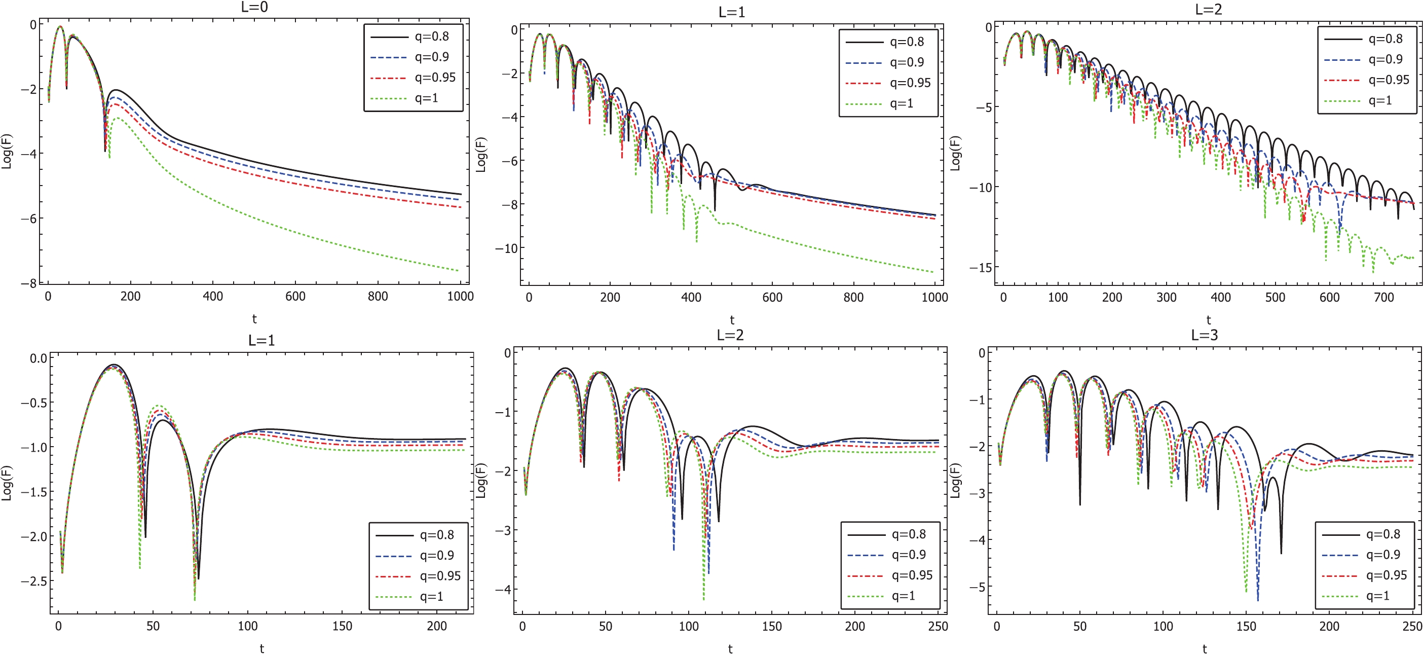
Figure 6. (color online) The calculated temporal evolution of the scalar (top row) and Dirac (bottom row) perturbations as the mass of the black hole approaches that of a purely magnetic one (
$ m = 0 $ ) for Case 1 with$ r_p = 1 $ . Here, the mass parameter$ m\to 0^+ $ from above as$ q\to 1^- $ from below. -
To summarize, in this study we investigated the scalar and Dirac quasinormal modes of the black hole solutions in the STGB theory. The calculations were carried out using both the WKB approximation and the finite difference method. The black hole solution is relevant as it is one of the first novel analytic solutions recently proposed in extended STGB gravity. While possessing a nonvanishing magnetic charge, the metric is capable of describing black holes with distinct characteristics by assuming different values of the ADM mass and the magnetic charge. Our analyses were focused on two specific types of metrics based on distinct features of their horizon structures. Additionally, quasinormal modes for purely magnetic black holes were investigated using a vanishing black hole mass parameter. The properties of the obtained complex frequencies were analyzed and compared to their counterparts in general relativity, and subsequently, the stability of the metric was addressed.
Scalar and Dirac quasinormal modes of scalar-tensor-Gauss-Bonnet black holes
- Received Date: 2021-10-20
- Available Online: 2022-04-15
Abstract: This study explores the scalar and Dirac quasinormal modes pertaining to a class of black hole solutions in the scalar-tensor-Gauss-Bonnet theory. The black hole metrics in question are novel analytic solutions recently derived in the extended version of the theory, which effectively follows at the level of the action of string theory. Owing to the existence of a nonlinear electromagnetic field, the black hole solution possesses a nonvanishing magnetic charge. In particular, the metric is capable of describing black holes with distinct characteristics by assuming different values of the ADM mass and the magnetic charge. This study investigates the scalar and Dirac perturbations in these black hole spacetimes; in particular, we focus on two different types of solutions, based on distinct horizon structures. The properties of the complex frequencies of the obtained dissipative oscillations are investigated, and the stability of the metric is subsequently addressed. We also elaborate on the possible implications of this study.


 DownLoad: