


 Abstract
 HTML
HTML Reference
 Related
 PDF
PDF


 DownLoad:


-
Many properties of atomic nuclei are very sensitive to their binding energy (or mass), such as half-lives and reaction rates. Therefore, physicists need to refine the theoretical model of the nucleus as much as possible to reproduce the experimental mass of the nucleus and to achieve the highest possible accuracy in predicting the nuclear mass. In 1932, the existence of the neutron was experimentally confirmed, and later it was proposed that a nucleus consists of positively charged protons and uncharged neutrons. Protons and neutrons (collectively known as nucleons) are bound to a very small volume, and thus begin the study of the structure of the nucleus. Because nucleus and nucleons are at the Fermi scale, it is believed that nucleons are closely arranged in the nucleus, so the liquid-drop model (LDM) of the nucleus was proposed. The LDM was first proposed by Gamow, then Weizsäcker and Bethe proposed a semi-empirical formula for calculating the binding energy of nuclei [1, 2]. Although such a description is approximate, it provides the basis for a more accurate description of the binding energy of the nucleus.
The LDM of the nucleus has been a great success in many ways, including describing fission of the nucleus. But many of the experimental data cannot be explained by the LDM. It is found that, similar to the change of atomic properties with the number of electrons in the atom, there are magic numbers in the properties of the nucleus with the number of neutrons and protons. This means that one nucleon in the nucleus moves in a different orbit in the mean field provided by the other nuclei. The magic number of protons and neutrons in the nucleus is successfully explained by the spherical simple harmonic oscillator potential with strong spin orbital coupling terms [3, 4]. This model can also explain the spin and parity of the ground state of the nucleus, as well as some experimental data of the electromagnetic transition from the excited state to the ground state of the nucleus. This is the shell model of the nucleus. M.G. Mayer and J.H.D. Jensen founded the shell model in 1949 [3, 4], for which they shared with Wigner the 1963 Nobel Prize in Physics.
The shell model can well reflect the shell structure of the nuclear energy levels, and can explain the magic numbers in experiments by the single particle motion in the mean field. The order of single particle energy levels and the phenomenon of shell splitting are explained. However, the shell model has some limitations and the reliability of the extrapolation has yet to be verified.
Combining the advantages of these two models, Strutinsky proposed a method of calculating shell corrections [5, 6]. Based on this method, macroscopic–microscopic models (MMM) are developed. MMM mainly include the Finite-range droplet model (FRDM) [7, 8], the Koura–Tachibana–Uno–Yamada mass formula (KTUY) [9], Lublin Strasbourg drop (LSD) [10], and the Weizsäcker–Skyrme (WS) mass formula (WS3.2 [11], WS3.3 [12], WS3.6 [13] and WS4 [14]). These models help us understand the nature of the strong nuclear force. However, we still cannot precisely calculate many questions about the structure of atomic nuclei, such as: How to determine the center of the superheavy stable island? How to calculate the magic number away from the beta stable line? What are the limits of nuclear existence? In addition to these problems, the mass of the nucleus is also very important in the study of nuclear astrophysics. It is difficult to answer these questions at present, because we need to predict unknown nuclei. The results of these models tend to be consistent in the known regions of the nucleus, but there are usually serious differences when they are far away from the known regions [15]. This may be because the shell correction energy calculation method is not applicable in some regions. It may also be because the current model ignores some unknown physical effects.
In recent years, artificial neural networks (ANN) have been widely used in various fields and successfully solved many complex problems [16–29]. The advantage of the NN approach is that there is no need to give an explicit relationship between the input and output data. ANN has the ability to learn and construct models of non-linear and complex relationships. The main purpose of this study is to demonstrate the success of an ANN in describing the energy of the ground state of unknown nuclei with known data.
In this paper we consider increasing the number of valence nucleons and the number of holes based on spherical shell closure in the nucleus as input quantities to reproduce the effect of the rise and fall of the binding energy of the nucleus. New nuclear binding energies can be verified in AME2020. The two neutron separation energies of the nuclei synthesized recently at the RIKEN RI Beam Factory are also calculated [30].
-
In MMM, the binding energy of the nucleus is expressed in two parts: the macroscopic liquid-drop part and the microscopic shell correction part. The simplest macroscopic expression is derived from the LDM, which can well explain the variation of nuclear binding energy except for a small deviation. According to the Strutinsky energy theory, the fluctuation of nuclear binding energy is provided by shell correction energy. Based on this idea, we also express the binding energy of the nucleus as the sum of the two parts of the energy
B(Z,A)NNLDM=ELDM(Z,A)+δBNNLDM.
(1) Unlike normal MMM, the macroscopic part of the energy does not take into account the deformation of the nucleus. Instead, the deformation energy, the shell correction energy and other energies are obtained using the NN approach. The energy of the liquid-drop can be expressed as
ELDM=aV(1+kVI2)A+aS(1+kSI2)A2/3+aCZ2A1/3(1−Z−2/3)+c12−|I|2+|I|AI2A+apairA−1/3δnp,
(2) where Z and A are the proton and mass numbers, respectively.
I=(A−2Z)/A is the charge-asymmetry parameter of the nucleus. The meanings of the terms in the formula are volume energy, surface energy, Coulomb energy, symmetric energy and average pair energy.δnp is expressed as [11]δnp={2−|I|,foreven−Z,even−N,|I|,forodd−Z,odd−N,1−|I|,forodd−Z,even−NandN>Z,1−|I|,foreven−Z,odd−NandN<Z,1,forodd−Z,even−NandN<Z,1,foreven−Z,odd−NandN>Z.
The parameters in Eq. (2) are obtained by fitting the binding energy in AME2016 [31]. We select 2314 nuclei with the number of protons and neutrons greater than or equal to 8 and the error of mass measurement less than or equal to 150 keV [32]. The fitting results are listed in Table 1. It can be seen that the root-mean-square deviation (RMSD) after fitting is 2.385 MeV. In Fig. 1, we use black solid circles to represent the deviation between the binding energy calculated by the LDM and the experimental values. This deviation is small relative to the total binding energy. But for the study of nuclear physics, such as nuclear astrophysics, nuclear reactions, decay energy of the nucleus and so on, such precision is far from enough. Next, we will introduce a NN approach to improve the precision of the LDM.
Parameter Value aV 
−15.6670 kV 
2.0219 aS 
18.4334 kS 
−3.1785 aC 
0.7153 c1 
44.5756 apair 
−6.8522 σ/MeV 2.385 Table 1. Model parameters of the LDM.
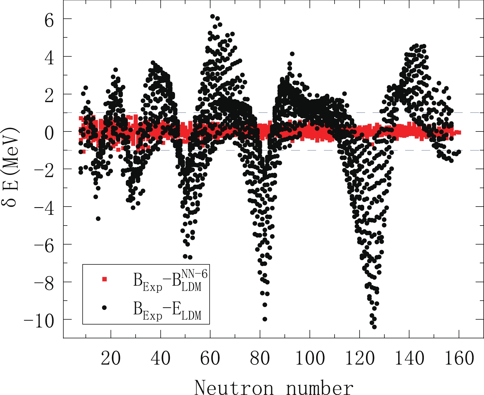
Figure 1. (color online) Deviation of theoretical calculation of binding energy from experimental values. Black solid circles are the deviation between the LDM result and the experimental value, and red solid squares are the modified results using the NN approach.
The ANN approach is a mathematical model that simulates brain function. A neuron takes one input, performs some mathematical operation, and then produces an output. In our calculation, we use a feedforward neural network. Feedforward neural networks adopt a unidirectional multi-layer structure. Each layer contains several neurons. In this NN model, each neuron can receive the signal from the previous layer and produce output to the next layer.
In an NN approach for nuclear binding energy, there are usually two input neurons, the number of protons Z and the number of nucleons A [22]. As for the LDM, the results can be approximated by the MMM after training. To get more accurate results, more physical information needs to be included in the input terms of the NN approach. In Ref. [23], the distance between the proton and neutron to the nearest magic number is taken into account in the input neurons. In Ref. [24], the pairing and shell effects are added to the input neurons, producing better results. It can be seen from literature that better results can be obtained by adding effective information as input neurons.
In Refs. [23, 24], only the shell contributions closest to the proton and neutron magic numbers are considered in the input neurons. But we think that between the two shells, the previous magic number and the next magic number both contribute to the energy of the nucleus. So in this contribution, the NN model is constructed with an input layer including six input neurons (proton number Z, mass number A, valence nucleus and hole number of neutrons (
|N−N0| and|N1−N| , and valence nucleus and hole number of protons|Z−Z0| and|Z1−Z| ), a hidden layer, and an output layer (δBNNLDM ).Z0 (8, 20, 50 and 82) andZ1 (20, 50, 82 and 126) here represent the number of protons in a given nucleus at the radius of the last magic number and the next magic number.N0 (8, 20, 50, 82 and 126) andN1 (20, 50, 82, 126 and 184) are the same numbers for neutrons. For example, for5626Fe30 , the inputs are, in turn 26, 56, 10 (30-20), 20 (50-30), 6 (26-20) and 24 (50-26). Since there is no prior indication to determine the number of neurons H in the optimal hidden layer, some considerations are used to determine the optimal choice. After many attempts, the number of neurons in the hidden layer was set at 40. The output layer of the NN model contains a neuron that represents the expected deviation of the nuclear binding energy. The structure of the NN model in this study is shown in Fig. 2.
Figure 2. (color online) A feedforward neural network consisting of six input neurons, a hidden layer and an output neuron.
We can use a function that expresses the relationship between the input and output for an ANN with a vector input x (
x1,x2,...,x6 ) and an output scalar y. It can be written as [22]:y=a+H∑j=1bjtanh(cj+n∑i=1djixi).
(3) where the free parameters are
ω=(a,bj,cj,dji) ; H is the number of neurons in the hidden layer; n is the input unit number;xi is the ith input unit;dji is the weight parameter between the ith input unit and the jth hidden neuron:cj is the bias of the jth hidden neuron;bj is the weight parameter between the jth hidden neuron and the output neuron; and a is the bias of the output neuron. For the six input variables, the function in Eq. (3) has 1 + (2+n)H parameters.Our goal is to obtain the minimum RMSD, so weights and biases need to be adjusted during training. In the learning stage of this work, we used a back propagation algorithm with Levenberg–Marquardt (LM) to change the connections between neurons so as to obtain the consistency between the neural network output and the expected output [33-35]. The LM algorithm is an iterative algorithm that can be used to solve the least square problem. The weight calculation formula of LM is as follows:
ωi+1=ωi−(JTiJi+μiI)−1JTiei,
(4) where
wi+1 is a trial solution estimated by thei th iteration solution. J is the Jacobian matrix of output error. I is the identity matrix. μ is a learning parameter (so called LM parameter). LM parameters have good operability and controllability, making the algorithm more stable and reliable. Now we can train the difference between the binding energy of the LDM and the experimental values. To illustrate the advantages of the six inputs (marked asδBNN−6LDM ), we also compare the results using four input neurons (there are three cases with four inputs: ①Z,A,Z−Z0,N−N0 , marked asδBNN−4LSLDM ; ②Z,A,Z1−Z, N1−N, marked asδBNN−4NSLDM ; ③Z,A,min(Z−Z0,Z1−Z), min(N−N0,N1−N) , marked asδBNN−4LDM ) and using two inputs (Z, A, marked asδBNN−2LDM ), which will be discussed in detail in the next section. -
Based on the previous instructions, we can now calculate the binding energy of the nuclei using the NN approach. Previously, we used 2314 nuclei experimental data from AME2016 to fit the parameters of Eq. (2). Using the NN method to train, the data should be divided into two parts, a learning set and a verification set. We randomly selected 414 experimental data as the verification set, and the remaining 1900 data as the learning set. The effect of hyperparameters can be removed by human adjustment. When the hidden layer neurons are fixed, we can tune the neural network model by adjusting the learning rate and the number of training sessions. For different input neurons, we can always find a suitable set of hyperparameters, but these hyperparameter sets are different. When the minimum root mean square deviation of the validation group occurs during the training process, the result at this point is considered to be the best result, rather than the minimum overall RMSD. This prevents over-fitting results. It should be noted that we have tried random selection several times and found little change. Here's the best one.
After using the NN approach, the RMSD of the LDM decreased significantly, especially when six input neurons were considered. The RMSD decreased from 2.385 to 0.203 MeV. The difference between the experimental binding energy and the corresponding calculated binding energy is shown in Fig. 1. In Table 2, we list the results of the NN method learning for the five variable input sets. From Table 2, we can clearly see that it is not sufficient to consider the effect of only one magic number on the shell correction. In all cases, the results with four inputs are not as good as with six inputs. We also show in Figs. 3–5 for each case how much the NN method results deviated from the experimental values. From Fig. 3 we can see, for nuclei near the magic number and nuclei in the light nucleus area, when only using the proton number and the mass number as input neurons in the NN method, the effect of the correction is poor. The reason is that shell effects are not taken into account. This situation is improved after considering the shell effect. From Fig. 4, we can see that the results have significantly improved. But there are still a lot of highly deviated nuclei in the light nucleus area. This is also a problem that MMM needs to solve. The present results can be significantly improved by using the NN method. Table 3 gives the accuracy of the description of the experimental masses by each of the models for five regions of nuclei: global (
Z,N⩾8 ), light (8⩽Z<28,N⩾8 ), medium-I (28⩽Z<50 ), medium-II (50⩽Z<82 ), and heavy (Z⩾82 ) nuclei.Model σpre /MeV
σNN /MeV
Δσ (%) Learning set BNN−2LDM 
2.388 0.383 83.96 BNN−4LSLDM 
2.388 0.235 90.16 BNN−4NSLDM 
2.388 0.231 90.33 BNN−4LDM 
2.388 0.216 90.95 BNN−6LDM 
2.388 0.196 91.79 Validation set BNN−2LDM 
2.375 0.386 83.75 BNN−4LSLDM 
2.375 0.275 88.42 BNN−4NSLDM 
2.375 0.255 89.26 BNN−4LDM 
2.375 0.246 89.64 BNN−6LDM 
2.375 0.231 90.27 Table 2. RMSD (MeV) of binding energy in light nuclei region calculated by different models.

Figure 3. (color online) Deviation with two input neurons.

Figure 5. (color online) Deviation with six input neurons.

Figure 4. (color online) Deviation of three results with four input neurons.
Model LDM BNN−2LDM 
BNN−4LSLDM 
BNN−4NSLDM 
BNN−4LDM 
BNN−6LDM 
WS4 [14] FRDM [8] KTUY [9] Global RMSD 2.385 0.384 0.242 0.236 0.221 0.203 0.288 0.584 0.704 Light RMSD 1.58 0.86 0.44 0.42 0.41 0.35 0.42 1.11 0.69 Medium-I RMSD 2.47 0.35 0.25 0.24 0.23 0.22 0.30 0.62 0.78 Medium-II RMSD 2.32 0.21 0.18 0.17 0.15 0.15 0.25 0.37 0.54 Heavy RMSD 2.79 0.25 0.15 0.16 0.15 0.13 0.24 0.37 0.88 Table 3. RMSD (MeV) calculated for the global (
Z,N⩾8 ), light (8⩽Z<28,N⩾8 ), medium-I (28⩽Z<50 ), medium-II (50⩽Z<82 ), and heavy (Z⩾82 ) nuclei, with the use of the specified models.One can see in Table 3 that for each region of the nuclear chart, the RMSD changes quite strongly from one model to another. A strong dependence of the accuracy of the description of the mass on the region of nuclei considered is obtained for each model. In all regions considered, the best accuracy is obtained by the
BNN−6LDM . One also can see similar patterns to the MMM of the shell correction calculated by the Strutinsky method. The improved result of the NN method for heavy nuclei is more obvious. If the shell effect is not considered in the input neurons, the correction results in the light nucleus region are poor. Different considerations in input would bring different results. From Table 3, we can clearly find that the shell closer to the nucleus has a greater impact on the nucleus, which is in line with the physical situation. However, if the input neurons are also considered to be a more distant shell, the results can be improved.Since the correction results of the NN method have such high accuracy for nuclei with known experimental binding energy, we should also verify the reliability of the NN method's extrapolation. Recently, the RIKEN RI Beam Factory used the time-of-flight magnetic rigidity technique to direct mass measurements of neutron-rich scandium, titanium and vanadium isotopes around the neutron number 40. The experimental results show that the two-neutron separation energy near 62Ti is increased compared with adjacent nuclei. In Ref. [30], we can find that the LZU model [36] has a slightly lower description of the two-neutron separation energy near 62Ti.
WS4RBF [14] also gives a similar result to LZU. In WS-type model [11–14, 36], the macroscopic part is expressed asELD∏(1+bkβ2k) and the microscopic part is the shell correction calculated by the Strutinsky method. The above parabolic approximation to the change of macroscopic energies withβk(k=2,3....) is acceptable near the ground state. In Ref. [21], R. Utama used a Bayesian NN approach to refine the Duflo–Zuker (DZ) model and the Hartree–Fock–Bogoliubov (HFB) model. The two-neutron separation energies in 61Ti and 62Ti are also smaller than the experimental values in DZ-BNN and HFB-BNN [21]. To verify the extrapolation ability of the NN method proposed in this paper, in addition to the RMSD, we also calculated the double neutron separation energy measured in Ref. [30]. The result of the calculation is shown in Fig. 6. As we can see in Fig. 6, compared with several other methods, NN-6 has a clear advantage, both in terms of trend and value. We have therefore chosen to compare the results of the two-neutron separation energy calculated by NN-6 with those of the LZU model. The results are plotted in Fig. 7. The experimental results and error bars are given in solid circles. The settlement result of the NN method is a solid square, and the dotted line represents the calculation result of the LZU model. From Fig. 7, we can clearly see that the computational results of the NN method reproduce the experimental values very well, especially in 61Ti and 62Ti. It should be noted that there is a large error in the experimental two neutron separation energy of 60Sc, and our result also has a large deviation from the experimental result. We believe that the shell effect like 62Ti should occur when the neutron number approaches N = 40 and scandium is no exception. Therefore, we believe that more accurate experimental measurement is needed for 60Sc. Other than that, almost all the other data falls within the error bar. We also listed the comparison between the binding energy of Ti in Ref. [30] and the calculation results of different models in Table 4. It can be seen that the trained NN model gives the best results.
Figure 6. (color online) Two-neutron separation energy calculated by using the different NN approaches compared with the results in Ref. [30].
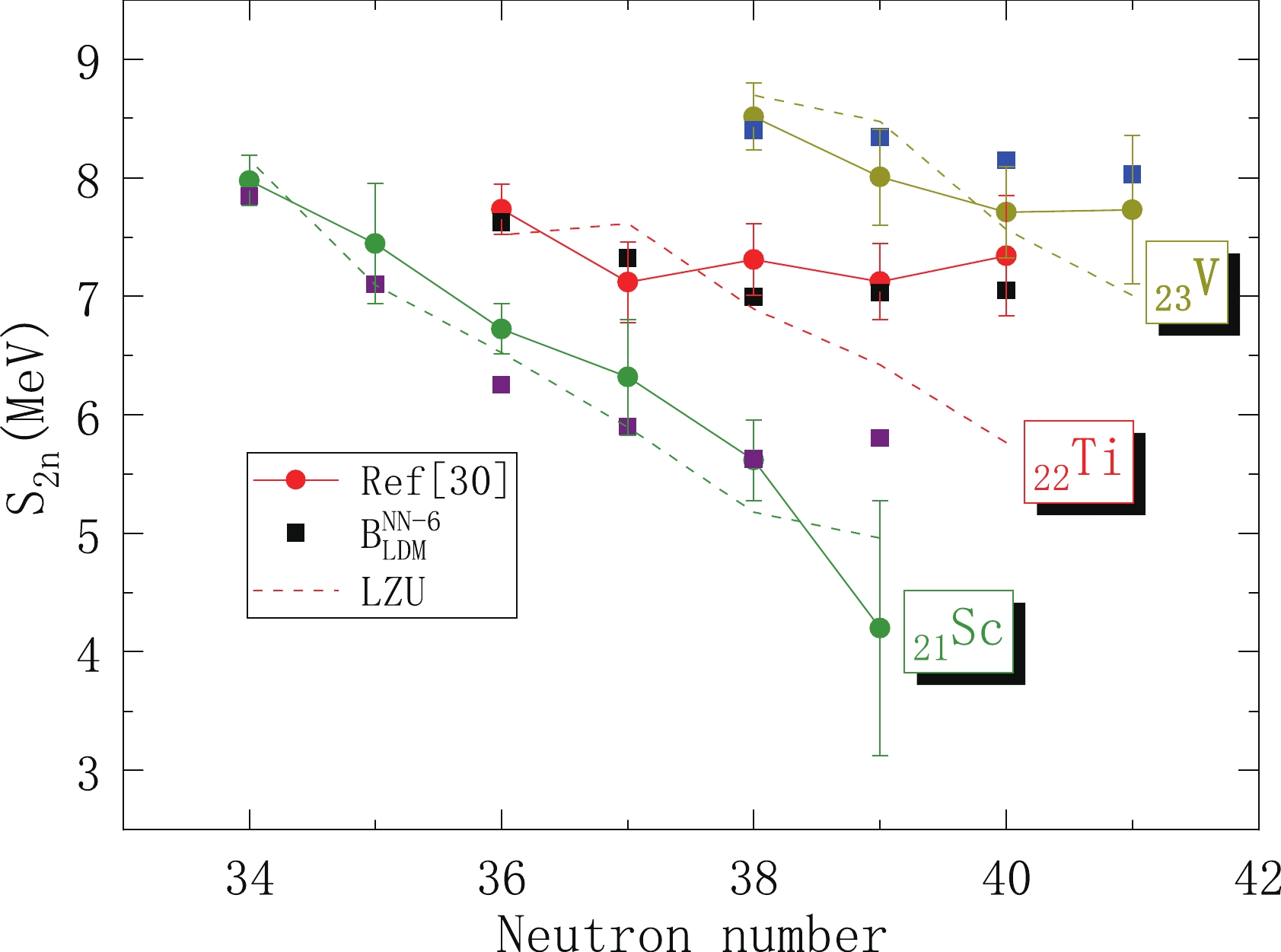
Figure 7. (color online) Two-neutron separation energy calculated by using the NN approach compared with the results in Ref. [30]. The solid circle is the experimental value in Ref. [30], the solid square is the calculation result of the work in this paper, and the dashed line is the calculation result of the LZU model. Different colors are used to represent different isotopic chains.
Model Ref. [30] AME2016 BNN−6LDM 
WS4 LZU 62Ti 
496.51 495.69 496.12 495.03 495.09 61Ti 
491.32 491.48 491.32 491.10 491.27 60Ti 
489.17 489.42 489.07 489.37 489.33 59Ti 
484.20 484.51 484.30 484.99 484.84 58Ti 
481.87 482.04 482.08 482.75 482.44 Table 4. Comparison of Ti isotopic chain binding energies (MeV) calculated by different models.
In addition, the latest quality assessment data, AME2020 [37], has been published. To further verify whether the work in this paper has extrapolation ability, we selected 78 updated nuclear binding energies from AME2020. The selected nuclei are either marked with
# (value and uncertainty derived not from purely experimental data, but at least partly from the trends from the mass surface) or have a deviation greater than 150 keV in AME2016. Similar to the previous discussion, we classified these nuclei into global (Z,N⩾8 ), light (8⩽Z<28, N⩾8 ), medium-I (28⩽Z<50 ), medium-II (50⩽Z<82 ), and heavy (Z⩾82 ) nuclei. ForBNN−6LDM , their RMSD were global nuclei (78) 0.455 MeV, light nuclei (23) 0.607 MeV, medium-I nuclei (11) 0.323 MeV, medium-II nuclei (28) 0.424 MeV and heavy nuclei (16) 0.303 MeV. ForBNN−2LDM ,BNN−4LSLDM ,BNN−4NSLDM andBNN−4LDM , their RMSD of global nuclei (78) were 0.677, 0.513, 0.426 and 0.605 MeV, respectively. Although the accuracy of the prediction is not as high as previous predictions, the results are acceptable. These results prove that the prediction of the modified model by the NN method is relatively reliable in the region near the known nucleus.NN-6 has more parameters. In order to eliminate the influence of parameter number, we increase the number of hidden neurons in NN-4 (H = 54). In this way, NN-6 and NN-4 (H = 54) are close in number of parameters, and the results are calculated and compared (the data in parentheses are the results for NN-6). For NN-4 (H = 54), the total RMSD is 0.209 (0.203) MeV, the RMSD of the training set is 0.201 (0.196) MeV and the RMSD of the validation set is 0.241 (0.231) MeV, 0.39 (0.35) MeV for the light nucleus region, 0.21 (0.22) MeV for Medium-I, 0.15 (0.15) MeV for Medium-II, and 0.14 (0.13) MeV for the heavy nucleus region. For the 78 nuclei added in AME2020, the RMSD is 0.564 (0.455) MeV. The computational results show that increasing the number of hidden layer neurons does reduce the total RMSD. Although the bias between the validation and training sets becomes larger, it is within an acceptable range. The extrapolation results also improved, but the results for the dual neutron separation energy were still poor. Even if the number of parameters is close, NN-6 has better extrapolation results with lower RMSD, which may be the advantage of using more input neurons.
However, if the inferred distance is too far from the known region, new physical effects may be generated, which are hidden in the unknown region and therefore cannot be detected by training the NN model with the known data. The calculation results of α decay energy from superheavy nuclei illustrate this point. In Ref. [38], the experimental values of alpha decay energy for 44 superheavy nuclei are listed. Neither these superheavy parent nuclei nor their decayed daughter nuclei are among the 2314 nuclei we used before. We present the comparison of the calculated results with the experimental values in Table 5. As can be seen from Table 5, the calculated results are relatively accurate when the proton number is less than 112, but when the proton number is greater than or equal to 112, the results show a large deviation. The reason may be that not enought data of superheavy nuclei is included in the training, and the maximum number of protons among the 2314 nuclei involved in the training is 110. Thus, it can be seen that the correction results of the NN method depend on the available experimental data. More data facilitates the training results and allows more accurate prediction of the binding energy of nuclei near known regions.
Z A Qα (Our work)
Qα (Ref. [38])
δ 118 294 12.47 11.82 0.65 117 294 12.06 11.18 0.88 117 293 12.44 11.32 1.12 116 293 11.95 10.71 1.24 116 292 12.36 10.78 1.58 116 291 12.64 10.89 1.75 116 290 12.80 11.00 1.80 115 290 12.41 10.41 2.00 115 289 12.49 10.49 2.00 115 288 12.47 10.65 1.82 115 287 12.38 10.76 1.62 114 289 12.06 9.98 2.08 114 288 12.07 10.07 2.00 114 287 11.97 10.17 1.80 114 286 11.83 10.35 1.48 114 285 11.72 10.56 1.16 113 286 11.37 9.79 1.58 113 285 11.21 10.01 1.20 113 284 11.12 10.12 1.00 113 283 11.10 10.38 0.72 113 282 11.16 10.78 0.38 112 285 10.70 9.32 1.38 112 283 10.49 9.66 0.83 112 281 10.63 10.45 0.18 111 282 9.85 9.16 0.69 111 281 9.92 9.41 0.51 111 280 10.08 10.15 −0.07 111 279 10.28 10.53 −0.25 111 278 10.49 10.85 −0.36 110 281 9.20 8.85 0.35 110 279 9.50 9.85 −0.35 110 277 10.00 10.71 −0.71 109 278 8.91 9.58 −0.67 109 276 9.47 10.10 −0.63 109 275 9.74 10.48 −0.74 109 274 9.99 10.20 −0.21 108 275 8.92 9.45 −0.53 108 273 9.50 9.67 −0.17 107 274 8.37 8.94 −0.57 107 272 8.97 9.21 −0.24 107 271 9.23 9.42 −0.19 107 270 9.46 9.06 0.40 106 271 8.44 8.67 −0.23 106 269 8.95 8.63 0.32 Table 5. Comparison of α decay energy calculated using the NN method with experimental values.
-
In summary, we have used the NN method to improve the nuclear mass prediction of the LDM. As the number of effective neurons in the input increases, the results become more accurate. The NN method with six input neurons has been able to reduce the RMSD of the LDM from 2.385 to 0.203 MeV. The six input neurons mainly modify the nuclear binding energy between the shells. This shows that this method is a very useful tool for further improving the precision of quality models. In order to verify the prediction ability of the NN method, the double neutron separation energy measured in the recent experiment was selected, and the results showed that the results using the NN fell within the error bar of the experiment. This suggests that if the NN method contains more physical features, the prediction is better not only in known regions, but also in unknown regions far from the β stable line. By partitioning the nuclei into groups, the improvement of the NN approach is more obvious for nuclei in the heavy nuclear region. However, from the results of calculating the α decay energy of superheavy nuclei, this method is currently not applicable to large-scale extrapolation.
A reliable neural network approach provides us with a way to find the super-heavy stable island, which is the plate we have been looking for. This work is in progress. In addition, the NN method can also be used to improve the properties of other nuclei, such as α decay half-life, nuclear charge radius and so on.
Table 1.
Model parameters of the LDM.
| Parameter | Value |
| −15.6670 |
| 2.0219 |
| 18.4334 |
| −3.1785 |
| 0.7153 |
| 44.5756 |
| −6.8522 |
| σ/MeV | 2.385 |


 DownLoad: