


 Abstract
 HTML
HTML Reference
 Related
 PDF
PDF


-
In recent years, an increasing number of heavy baryons have been confirmed by the Belle, LHCb, and CDF collaborations, and the spectra of the charm and bottom baryon families have become increasingly abundant. For excited bottom baryons in particular, scientists have achieved significant progress in theoretical and experimental studies in recent years, such as for
$ \Lambda_{b}(5912) $ ,$ \Lambda_{b}(5920) $ [1, 2],$ \Lambda_{b}(6072) $ [3, 4],$ \Xi_{b}(6227) $ [5–7], and$ \Xi_{b}(6100) $ [8]. In 2019, the LHCb collaboration reported the discovery of two bottom baryon states,$ \Lambda_{b}(6146)^{0} $ and$ \Lambda_{b}(6152)^{0} $ , by analyzing the$ \Lambda_{b}^{0}\pi^{+}\pi^{-} $ invariant mass spectrum from$ pp $ collisions [9]. The measured masses and widths are$ \begin{aligned}[b] m_{\Lambda_{b}(6146)^{0}}=&6146.17\pm0.33\pm0.22\pm0.16 ~~{\rm{MeV}}, \\\Gamma_{\Lambda_{b}(6146)^{0}}=&2.9\pm1.3\pm0.3 ~~{\rm{MeV}}, \\ m_{\Lambda_{b}(6152)^{0}}=&6152.51\pm0.26\pm0.22\pm0.16 ~~{\rm{MeV}}, \\\Gamma_{\Lambda_{b}(6152)^{0}}=&2.1\pm2.1\pm0.8\pm0.3 ~~{\rm{MeV}}. \end{aligned}$

By studying their strong decays using quark model or
$ ^{3}P_{0} $ model, scholars interpreted these two states as a$ \Lambda_{b}(1D) $ doublet [6, 10–13]. Before this observation, different collaborations predicted the masses of this doublet using the quark model [14–17], whose results were not consistent with each other and with experiments, and they require further confirmation using different theoretical methods and models.Very recently, the LHCb collaboration reported the observation of two new excited
$ \Xi_{b} $ states in the$ \Lambda_{b}K^{-}\pi^{+} $ mass spectrum [18]. The measured masses and widths were$\begin{aligned}[b] m_{\Xi_{b}(6327)}=&6327.28^{+0.23}_{-0.21}({\rm{stat}})\pm0.08 ({\rm{syst}}) \\&\pm0.24(m_{\Lambda{b}}) ~{\rm{MeV},}~\;\;\;\; \Gamma_{\Xi_{b}(6327)}<2.20 ~{\rm{MeV},}~ \\ m_{\Xi_{b}(6333)}=&6332.69^{+0.17}_{-0.18}({\rm{stat}})\pm0.03 ({\rm{syst}}) \\&\pm0.22(m_{\Lambda{b}}) ~{\rm{MeV},}~\;\;\;\; \Gamma_{\Xi_{b}(6327)}<1.55 ~{\rm{MeV}.}\end{aligned} $

By comparing with the quark-model predictions[6, 10], Chen et al. interpreted these two states as a
$ 1D $ ($ \Xi_{b} $ ) doublet with$ J^{P}={3}/{2}^{+} $ and$ {5}/{2}^{+} $ .Many theoretical methods and models have been used over the past decades to investigate bottom baryons, including the quark model [12, 14–16, 19–41], heavy hadron chiral perturbation theory [42–47],
$ ^{3}P_{0} $ decay model [48–54], lattice quantum chromodynamics (QCD) [55–58], light cone QCD sum rules [59–66], and QCD sum rules [67–79]. For more discussions on bottom baryon states, please consult Refs. [17, 80–88] and the references therein. Through the efforts of theoretical and experimental physicists, some bottom baryon states have been observed and confirmed, such as$ \Xi_{b}(5797) $ [89],$ \Lambda_{b}(5620) $ [89],$ \Lambda_{b}(5912) $ [89],$ \Lambda_{b}(5920) $ [89], and$ \Lambda_{b}(6072) $ [3, 4], whose quantum numbers were determined to be 1S($ {1}/{2}^{+} $ ), 1S($ {1}/{2}^{+} $ ), 1P(${1}/{2}^{-} $ ), 1P($ {3}/{2}^{-} $ ), and 2S($ {1}/{2}^{+} $ ), respectively. However, the inner structures of the newly observed baryon states$ \Xi_{b}(6327) $ ,$ \Xi_{b}(6333) $ ,$ \Lambda(6146) $ , and$ \Lambda(6152) $ require further confirmation theoretically. The other bottom baryon states, such as the radially excited D-wave$ \Xi_{b} $ and$ \Lambda_{b} $ baryons, have not been observed.The QCD sum rule method has been proven to be the most effective non-perturbative method in studying the properties of mesons and baryons [70, 90–98], and it has been extended to studying multiquark states [99–106]. In our previous study, we systematically studied the D-wave charmed baryons
$ \Lambda_{c}(2860) $ ,$ \Lambda_{c}(2880) $ ,$ \Xi_{c}(3055) $ , and$ \Xi_{c}(3080) $ [71], the P-wave$ \Omega_{c} $ states,$ \Omega_{c}(3000) $ ,$ \Omega_{c}(3050) $ ,$ \Omega_{c}(3066) $ ,$ \Omega_{c}(3090) $ , and$ \Omega_{c}(3119) $ [107, 108], and the$ \Omega_{b} $ states,$ \Omega_{b}(6316) $ ,$ \Omega_{b}(6330) $ ,$ \Omega_{b}(6340) $ , and$ \Omega_{b}(6350) $ [109] using the method of QCD sum rules. As a continuation of our previous research, we study the$ 1D $ and$ 2D $ states of$ \Xi_{b} $ and$ \Lambda_{b} $ baryons with orbital excitations ($ L_{\rho},L_{\lambda})= $ ($ 0,2 $ ), ($ 2,0 $ ), and ($ 1,1 $ ). The motivation of this study was to further confirm the structures of$ \Lambda_{b}(6146) $ ,$ \Lambda_{b}(6152) $ ,$ \Xi_{b}(6327) $ , and$ \Xi_{b}(6333) $ , decode their excitation modes, and predict the masses and pole residues of$ 1D $ and$ 2D \Xi_{b} $ and$ \Lambda_{b} $ baryons.The remainder this paper is outlined as follows: in Sec. II, we first construct three types of interpolating currents for D-wave bottom baryons
$ \Lambda_{b} $ and$ \Xi_{b} $ ; in Sec. III, we derive QCD sum rules for the masses and pole residues of these states with spin-parity${3}/{2}^{+} $ and$ {5}/{2}^{+} $ from two-point correlation function; in Sec. IV, we present the numerical results and discussions; and Sec. V presents our conclusions. -
In the heavy quark limit, one heavy quark within a heavy baryon system is decoupled from two light quarks. Under this scenario, the dynamics of a heavy baryon state can be separated into two parts: the
$ \rho $ -mode, which is for the degree of freedom between two light quarks, and the$ \lambda $ -mode, which denotes the degree between the center of mass of diquarks and the heavy quark. In this diquark-quark model, the orbital angular momentum between the two light quarks is denoted by$ L_{\rho} $ , and the angular momentum between the light diquarks and heavy quark is denoted by$ L_{\lambda} $ . The D-wave ($ L=2 $ ) bottom baryon has three orbital excitation modes: ($ L_{\rho},L_{\lambda})=( $ $ 2,0 $ ), ($ 0,2 $ ), and ($ 1,1 $ ). The color antitriplet diquarks with quantum numbers of$ L_{\rho}=0 $ and$ s_{l}=0 $ can be expressed as$ \varepsilon^{ijk}q^{T}_{j}C\gamma_{5}q'_{k} $ , which has the spin-parity of$ J^{P}_{d}=0^{+}_{d} $ . The spin-parity of relative P-wave and D-wave are denoted as$ J_{\rho/\lambda}^{P}=L_{\rho/\lambda}^{P}=1_{\rho/\lambda}^{-} $ and$ 2_{\rho/\lambda}^{+} $ , respectively. If$ J_{b}^{P}=({1}/{2})_{b}^{+} $ is the spin-parity of b-quark, we can obtain the final states of D-wave bottom baryons according to direct product of angular momentum$ J^{P}= 0^{+}_{d}\bigotimes J_{\rho/\lambda}^{P}\bigotimes \frac{1}{2}_{b}^{+} $ .For the excitation mode (
$ L_{\rho},L_{\lambda} )=$ $(1,0 )$ , the P-wave diquark system with$ J^{P}=1^{-} $ can be constructed by applying a derivative between two light quarks:$ \begin{eqnarray} \epsilon^{ijk}\big[\partial^{\beta}q_{i}^{T}(x)C\gamma_{5}q'_{j}(x)-q_{i}^{T}(x)C\gamma_{5}\partial^{\beta}q'_{j}(x)\big]. \end{eqnarray} $

(1) Based on this, we introduce an additional derivative between the two light quarks in Eq. (1) to obtain the excitation mode of (
$ L_{\rho},L_{\lambda})= $ $ (2,0 )$ $ \begin{aligned}[b] &\epsilon^{ijk}\Big\{\big[\partial^{\alpha}\partial^{\beta}q_{i}^{T}(x)C\gamma_{5}q'_{j}(x)-\partial^{\beta}q_{i}^{T}(x)C\gamma_{5}\partial^{\alpha}q'_{j}(x)\big]\\&-\big[\partial^{\alpha}q_{i}^{T}(x)C\gamma_{5}\partial^{\beta}q'_{j}(x)-q_{i}^{T}(x)C\gamma_{5}\partial^{\alpha}\partial^{\beta}q'_{j}(x)\big]\Big\}. \end{aligned} $

(2) For the excitation mode (
$ L_{\rho},L_{\lambda})= $ $( 0,2) $ , we must apply two derivatives between the diquark system and b-quark field. It should be noted that the b-quark in the bottom baryon is static in the heavy quark limit. Thus,$ \overleftrightarrow{\partial}_{\mu} $ is reduced to$ \overleftarrow{\partial}_{\mu} $ when operating on the b-quark field, and the light diquark state with$ J^{P}=2^{+} $ is expressed as$ \begin{aligned}[b] \partial^{\alpha}\partial^{\beta}\big[\epsilon^{ijk}q_{i}^{T}(x)C\gamma_{5}q'_{j}(x)\big]=&\epsilon^{ijk}\big[\partial^{\alpha}\partial^{\beta}q_{i}^{T}(x)C\gamma_{5}q'_{j}(x)\\&+\partial^{\beta}q_{i}^{T}(x)C\gamma_{5}\partial^{\alpha}q'_{j}(x)\big] \\ & +\partial^{\alpha}q_{i}^{T}(x)C\gamma_{5}\partial^{\beta}q'_{j}(x)\\&+q_{i}^{T}(x)C\gamma_{5}\partial^{\alpha}\partial^{\beta}q'_{j}(x)\big]. \end{aligned} $

(3) For the (
$ L_{\rho},L_{\lambda} )=$ $ (1,1 $ ) state, we require an additional derivative between the P-wave diquark (Eq. (1)) and b-quark field:$ \begin{aligned}[b] &\partial^{\alpha}\epsilon^{ijk}\big[\partial^{\beta}q_{i}^{T}(x)C\gamma_{5}q'_{j}(x)-q_{i}^{T}(x)C\gamma_{5}\partial^{\beta}q'_{j}(x)\big]\\ =& \epsilon^{ijk}\big[\partial^{\alpha}\partial^{\beta} q_{i}^{T}(x)C\gamma_{5}q'_{j}(x)+\partial^{\beta}q_{i}^{T}(x)C\gamma_{5}\partial^{\alpha}q'_{j}(x)\\&-\partial^{\alpha}q_{i}^{T}(x)C\gamma_{5}\partial^{\beta}q'_{j}(x) - q_{i}^{T}(x)C\gamma_{5}\partial^{\alpha}\partial^{\beta} q'_{j}(x)\big]\Gamma_{\alpha\beta\mu\nu}c_{k}(x). \end{aligned} $

(4) Considering the symmetrization of the Lorentz indexes μ and ν, the light diquark state with (
$ L_{\rho},L_{\lambda})= $ $ (1,1 $ ) can be expressed in a simpler form:$ \begin{eqnarray} \epsilon^{ijk}\big[\partial^{\alpha}\partial^{\beta} q_{i}^{T}(x)C\gamma_{5}q'_{j}(x)- q_{i}^{T}(x)C\gamma_{5}\partial^{\alpha}\partial^{\beta} q'_{j}(x)\big]. \end{eqnarray} $

(5) Finally, we combine the above light diquark systems with the b-quark field to form
$ J^{P}={3}/{2}^{+} $ or$ {5}/{2}^{+} $ baryon states that have three excitation modes, ($ L_{\rho},L_{\lambda})= $ $ (2,0 $ ), ($ 0,2 $ ), and ($ 1,1 $ ). For more details about the construction of the interpolating currents of baryons, please consult Refs. [71, 72, 97]. We can now classify these constructed interpolating currents as follows:$\begin{aligned}[b] (L_{\rho},L_{\lambda})=\,&(0,2) ~~{\rm{for}} ~~ J^{1}_{\mu}/\eta_{\mu}^{1}(x) , J^{1}_{\mu\nu}/\eta_{\mu\nu}^{1}(x) , \\ (L_{\rho},L_{\lambda})=\,&(2,0) ~~{\rm{for}} ~~ J^{2}_{\mu}/\eta_{\mu}^{2}(x) , J^{2}_{\mu\nu}/\eta_{\mu\nu}^{2}(x) , \\ (L_{\rho},L_{\lambda})=\,&(1,1) ~~{\rm{for}} ~~ J^{3}_{\mu}/\eta_{\mu}^{3}(x) , J^{3}_{\mu\nu}/\eta_{\mu\nu}^{3}(x) ,\end{aligned} $

where
$ J_{\mu} $ ,$ \eta_{\mu} $ are for$ \Xi_{b} $ and$ \Lambda_{b} $ with quantum numbers$ {1}/{2}^{+} $ ;$ J_{\mu\nu} $ ,$ \eta_{\mu\nu} $ denote$ {3}/{2}^{+} \Xi_{b} $ and$ \Lambda_{b} $ baryons, respectively. The interpolating currents for different excitation modes ($ L_{\rho},L_{\lambda})= $ $( 0,2 $ ), ($ 2,0 $ ), and ($ 1,1 $ ) are denoted as$ J^{n} $ and$ \eta^{n} $ with$ n=1 $ ,$ 2 $ , and$ 3 $ , respectively, which can be expressed as$ \begin{aligned}[b] J_{\mu}^{1}(x)=&\epsilon^{ijk}\big[\partial^{\alpha}\partial^{\beta} q_{i}^{T}(x)C\gamma_{5}s_{j}(x)+\partial^{\alpha}q_{i}^{T}(x)C\gamma_{5}\partial^{\beta}s_{j}(x)\\&+\partial^{\beta}q_{i}^{T}(x)C\gamma_{5}\partial^{\alpha}s_{j}(x) \\& + q_{i}^{T}(x)C\gamma_{5}\partial^{\alpha}\partial^{\beta} s_{j}(x)\big]\Gamma_{\alpha\beta\mu}b_{k}(x),\\ J_{\mu}^{2}(x)=&\epsilon^{ijk}\big[\partial^{\alpha}\partial^{\beta} q_{i}^{T}(x)C\gamma_{5}s_{j}(x)-\partial^{\alpha}q_{i}^{T}(x)C\gamma_{5}\partial^{\beta}s_{j}(x)\\&-\partial^{\beta}q_{i}^{T}(x)C\gamma_{5}\partial^{\alpha}s_{j}(x) \\ & + q_{i}^{T}(x)C\gamma_{5}\partial^{\alpha}\partial^{\beta} s_{j}(x)\big]\Gamma_{\alpha\beta\mu}b_{k}(x) \\ J_{\mu}^{3}(x)=&\epsilon^{ijk}\big[\partial^{\alpha}\partial^{\beta} q_{i}^{T}(x)C\gamma_{5}s_{j}(x),\\&- q_{i}^{T}(x)C\gamma_{5}\partial^{\alpha}\partial^{\beta} s_{j}(x)\big]\Gamma_{\alpha\beta\mu}b_{k}(x), \end{aligned} $

(6) $ \begin{aligned}[b] \eta_{\mu}^{1}(x)=&\epsilon^{ijk}\big[\partial^{\alpha}\partial^{\beta} q_{i}^{T}(x)C\gamma_{5}q'_{j}(x)+\partial^{\alpha}q_{i}^{T}(x)C\gamma_{5}\partial^{\beta}q'_{j}(x)\\&+\partial^{\beta}q_{i}^{T}(x)C\gamma_{5}\partial^{\alpha}q'_{j}(x) \\ & + q_{i}^{T}(x)C\gamma_{5}\partial^{\alpha}\partial^{\beta} q'_{j}(x)\big]\Gamma_{\alpha\beta\mu}b_{k}(x), \\ \eta_{\mu}^{2}(x)=&\epsilon^{ijk}\big[\partial^{\alpha}\partial^{\beta} q_{i}^{T}(x)C\gamma_{5}q'_{j}(x)-\partial^{\alpha}q_{i}^{T}(x)C\gamma_{5}\partial^{\beta}q'_{j}(x)\\&-\partial^{\beta}q_{i}^{T}(x)C\gamma_{5}\partial^{\alpha}q'_{j}(x) \\ & + q_{i}^{T}(x)C\gamma_{5}\partial^{\alpha}\partial^{\beta} q'_{j}(x)\big]\Gamma_{\alpha\beta\mu}b_{k}(x), \\ \eta_{\mu}^{3}(x)=&\epsilon^{ijk}\big[\partial^{\alpha}\partial^{\beta} q_{i}^{T}(x)C\gamma_{5}q'_{j}(x)\\&- q_{i}^{T}(x)C\gamma_{5}\partial^{\alpha}\partial^{\beta} q'_{j}(x)\big]\Gamma_{\alpha\beta\mu}b_{k}(x), \end{aligned} $

(7) $ \begin{aligned} J_{\mu\nu}^{1}(x)=&\epsilon^{ijk}\big[\partial^{\alpha}\partial^{\beta} q_{i}^{T}(x)C\gamma_{5}s_{j}(x)+\partial^{\alpha}q_{i}^{T}(x)C\gamma_{5}\partial^{\beta}s_{j}(x)\\&+\partial^{\beta}q_{i}^{T}(x)C\gamma_{5}\partial^{\alpha}s_{j}(x) \\ & + q_{i}^{T}(x)C\gamma_{5}\partial^{\alpha}\partial^{\beta} s_{j}(x)\big]\Gamma_{\alpha\beta\mu\nu}b_{k}(x), \end{aligned} $

$ \begin{aligned} J_{\mu\nu}^{2}(x)=&\epsilon^{ijk}\big[\partial^{\alpha}\partial^{\beta} q_{i}^{T}(x)C\gamma_{5}s_{j}(x)-\partial^{\alpha}q_{i}^{T}(x)C\gamma_{5}\partial^{\beta}s_{j}(x)\\&-\partial^{\beta}q_{i}^{T}(x)C\gamma_{5}\partial^{\alpha}s_{j}(x) \\ & + q_{i}^{T}(x)C\gamma_{5}\partial^{\alpha}\partial^{\beta} s_{j}(x)\big]\Gamma_{\alpha\beta\mu\nu}b_{k}(x) \\ J_{\mu\nu}^{3}(x)=&\epsilon^{ijk}\big[\partial^{\alpha}\partial^{\beta} q_{i}^{T}(x)C\gamma_{5}s_{j}(x),\\&- q_{i}^{T}(x)C\gamma_{5}\partial^{\alpha}\partial^{\beta} s_{j}(x)\big]\Gamma_{\alpha\beta\mu\nu}b_{k}(x), \end{aligned} $

(8) $ \begin{aligned}[b] \eta_{\mu\nu}^{1}(x)=&\epsilon^{ijk}\big[\partial^{\alpha}\partial^{\beta} q_{i}^{T}(x)C\gamma_{5}q'_{j}(x)+\partial^{\alpha}q_{i}^{T}(x)C\gamma_{5}\partial^{\beta}q'_{j}(x)\\&+\partial^{\beta}q_{i}^{T}(x)C\gamma_{5}\partial^{\alpha}q'_{j}(x) \\ & + q_{i}^{T}(x)C\gamma_{5}\partial^{\alpha}\partial^{\beta} q'_{j}(x)\big]\Gamma_{\alpha\beta\mu\nu}b_{k}(x) \\ \eta_{\mu\nu}^{2}(x)=&\epsilon^{ijk}\big[\partial^{\alpha}\partial^{\beta} q_{i}^{T}(x)C\gamma_{5}q'_{j}(x)-\partial^{\alpha}q_{i}^{T}(x)C\gamma_{5}\partial^{\beta}q'_{j}(x)\\&-\partial^{\beta}q_{i}^{T}(x)C\gamma_{5}\partial^{\alpha}q'_{j}(x), \\ & + q_{i}^{T}(x)C\gamma_{5}\partial^{\alpha}\partial^{\beta} q'_{j}(x)\big]\Gamma_{\alpha\beta\mu\nu}b_{k}(x) \\\eta_{\mu\nu}^{3}(x)=&\epsilon^{ijk}\big[\partial^{\alpha}\partial^{\beta} q_{i}^{T}(x)C\gamma_{5}q'_{j}(x),\\&- q_{i}^{T}(x)C\gamma_{5}\partial^{\alpha}\partial^{\beta} q'_{j}(x)\big]\Gamma_{\alpha\beta\mu\nu}b_{k}(x), \end{aligned} $

(9) where
$ \Gamma_{\alpha\beta\mu} $ and$ \Gamma_{\alpha\beta\mu\nu} $ are the projection operatiors, whose explicit forms are:$ \begin{eqnarray} \Gamma_{\alpha\beta\mu}=(g_{\alpha\mu}g_{\beta\nu}+g_{\alpha\nu}g_{\beta\mu}-\frac{1}{2}g_{\alpha\beta}g_{\mu\nu})\gamma^{\nu}\gamma_{5}, \end{eqnarray} $

(10) $ \begin{aligned}[b] \Gamma_{\alpha\beta\mu\nu}=&g_{\alpha\mu}g_{\beta\nu}+g_{\alpha\nu}g_{\beta\mu}-\frac{1}{6}g_{\alpha\beta}g_{\mu\nu}-\frac{1}{4}g_{\alpha\mu}\gamma_{\beta}\gamma_{\nu}\\&-\frac{1}{4}g_{\alpha\nu}\gamma_{\beta}\gamma_{\mu}-\frac{1}{4}g_{\beta\mu}\gamma_{\alpha}\gamma_{\nu}-\frac{1}{4}g_{\beta\nu}\gamma_{\alpha}\gamma_{\mu} \\ & +\frac{1}{24}\gamma_{\alpha}\gamma_{\mu}\gamma_{\beta}\gamma_{\nu}+\frac{1}{24}\gamma_{\alpha}\gamma_{\nu}\gamma_{\beta}\gamma_{\mu}\\&+\frac{1}{24}\gamma_{\beta}\gamma_{\mu}\gamma_{\alpha}\gamma_{\nu}+\frac{1}{24}\gamma_{\beta}\gamma_{\nu}\gamma_{\alpha}\gamma_{\mu}. \end{aligned} $

(11) Note that we can select either the partial derivative
$ \partial_{\mu} $ or the covariant derivative$ D_{\mu} $ to construct the interpolating currents. The current with the covariant derivative is gauge invariant but blurs the physical interpretation of$ \overleftrightarrow{D}_{\mu} $ being the angular momentum. The current with the partial derivative$ \partial_{\mu} $ is not gauge invariant but manifests the physical interpretation of$ \overleftrightarrow{\partial}_{\mu} $ being the angular momentum. In the calculations with these two currents in QCD sum rules, the difference is that the current with the covariant derivative$ D_{\mu} $ emits a gluon at a interaction vertex. This gluon field contributes to the gluon condensate terms. Our research indicates that the contributions of these condensate terms from the vertex result in negligible difference in the final results [98]. Thus, we neglect the contributions from the vertex in gluon condensate terms and use the current with the partial derivative$ \partial_{\mu} $ as our interpolating currents. -
The first step of the analysis with QCD sum rules is to write down the following two-point correlation functions:
$ \begin{aligned}[b] \Pi_{\mu\nu}(p)&={\rm i}\int {\rm d}^{4}x{\rm e}^{{\rm i}p.x}\Big\langle0|T\Big\{J_{\mu}/\eta_{\mu}(x)\overline{J}_{\nu}/\overline{\eta}_{\nu}(0)\Big\} |0\Big\rangle,\\ \Pi_{\mu\nu\alpha\beta}(p)&={\rm i}\int {\rm d}^{4}x{\rm e}^{{\rm i}p.x}\Big\langle0|T\Big\{J_{\mu\nu}/\eta_{\mu\nu}(x)\overline{J}_{\alpha\beta}/\overline{\eta}_{\alpha\beta}(0)\Big\} |0\Big\rangle, \end{aligned} $

(12) where T is the time ordered product. The currents
$ J_{\mu}/\eta_{\mu}(0) $ and$ J_{\mu\nu}/\eta_{\mu\nu}(0) $ in these correlations couple potentially to$ 1D $ bottom states$ B_{{3}/{2}^{\pm}} $ and$ B_{{5}/{2}^{\pm}} $ , respectively, and couple also to$ 2D $ states$ B^{\prime}_{{3}/{2}^{\pm}} $ and$ B^{\prime}_{{5}/{2}^{\pm}} $ with the quantum numbers$ {3}/{2}^{+} $ and$ {5}/{2}^{+} $ :$ \begin{aligned}[b] \langle 0| J/\eta_{\mu}(0)|B^{(\prime)+}_{{3}/{2}}(p) \rangle=&\lambda^{(\prime)+}_{{3}/{2}}U^+_{\mu}(p,s), \\ \langle 0| J/\eta_{\mu\nu}(0)|B^{(\prime)+}_{{5}/{2}}(p) \rangle=&\lambda^{(\prime)+}_{{5}/{2}}U^+_{\mu\nu}(p,s), \end{aligned} $

(13) $ \begin{aligned}[b] \langle 0| J/\eta_{\mu}(0)|B^{(\prime)-}_{\frac{3}{2}}(p) \rangle=&\lambda^{(\prime)-}_{{3}/{2}}{\rm i}\gamma_{5}U^-_{\mu}(p,s),\\ \langle 0| J/\eta_{\mu\nu}(0)|B^{(\prime)-}_{{5}/{2}}(p) \rangle=&\lambda^{(\prime)-}_{{5}/{2}}{\rm i}\gamma_{5}U^-_{\mu\nu}(p,s). \end{aligned} $

(14) -
At the hadron level, a complete set of intermediate baryon states with the same quantum numbers as the current operators
$ J_{\mu}/\eta_{\mu}(x) $ ,$ J_{\mu\nu}/\eta_{\mu\nu}(x) $ ,$ {\rm i}\gamma_{5}J_{\mu}/\eta_{\mu}(x) $ , and$ {\rm i}\gamma_{5}J_{\mu\nu}/\eta_{\mu\nu}(x) $ are inserted into the correlation functions$ \Pi_{\mu\nu}(p) $ and$ \Pi_{\mu\nu\alpha\beta}(p) $ . After separating the pole terms of the lowest$ 1D $ and$ 2D $ states, we obtain the following results:$ \begin{aligned}[b] \Pi_{\mu\nu}(p)=&\left(\lambda^{+2}_{{3}/{2}}\frac{\not p+M_{{3}/{2}}^+}{M_{{3}/{2}}^{+2}-p^{2}}+\lambda^{-2}_{{3}/{2}}\frac{\not p-M_{{3}/{2}}^-}{M_{{3}/{2}}^{-2}-p^{2}}\right. \\&\left.+\lambda^{\prime+2}_{{3}/{2}}\frac{\not p+M^{\prime+}_{{3}/{2}}}{M_{{3}/{2}}^{\prime+2}-p^{2}}+\lambda^{\prime-2}_{{3}/{2}}\frac{\not p-M^{\prime-}_{{3}/{2}}}{M_{{3}/{2}}^{\prime-2}-p^{2}}\right) \\ &\times\left(-g_{\mu\nu}+\frac{\gamma_{\mu}\gamma_{\nu}}{3}+\frac{2p_{\mu}p_{\nu}}{3p^{2}}-\frac{p_{\mu}\gamma_{\nu}-p_{\nu}\gamma_{\mu}}{3\sqrt{p^{2}}}\right)+\cdots \\ =&\Pi_{{3}/{2}}(p^{2})(-g_{\mu\nu})+\cdots\\[-13pt] \end{aligned} $

(15) $ \begin{aligned}[b] \Pi_{\mu\nu}(p)=\left(\lambda^{+2}_{{5}/{2}}\frac{\not p+M_{{5}/{2}}^+}{M_{{5}/{2}}^{+2}-p^{2}}+\lambda^{-2}_{{5}/{2}}\frac{\not p-M_{{5}/{2}}^-}{M_{{5}/{2}}^{-2}-p^{2}}\right. \end{aligned} $

$ \begin{aligned}[b] &\left.+\lambda^{\prime+2}_{{5}/{2}}\frac{\not p+M^{\prime+}_{{5}/{2}}}{M_{{5}/{2}}^{\prime+2}-p^{2}}+\lambda^{\prime-2}_{{5}/{2}}\frac{\not p-M^{\prime-}_{{5}/{2}}}{M_{{5}/{2}}^{\prime-2}-p^{2}}\right) \\ &\times\Bigg[\frac{\widetilde{g}_{\alpha\mu}\widetilde{g}_{\beta\nu} +\widetilde{g}_{\alpha\nu}\widetilde{g}_{\beta\mu}}{2}-\frac{\widetilde{g}_{\alpha\beta}\widetilde{g}_{\mu\nu}}{5}\\&-\frac{1}{10}\left(\gamma_{\mu}\gamma_{\alpha}+\frac{p_{\alpha}\gamma_{\mu}-p_{\mu}\gamma_{\alpha}}{\sqrt{p^{2}}}-\frac{p_{\mu}p_{\alpha}}{p^{2}}\right) \widetilde{g}_{\beta\nu} \\ & -\frac{1}{10}\left(\gamma_{\mu}\gamma_{\beta}+\frac{p_{\beta}\gamma_{\mu}-p_{\mu}\gamma_{\beta}}{\sqrt{p^{2}}}-\frac{p_{\mu}p_{\beta}}{p^{2}}\right)\widetilde{g}_{\alpha\mu}\Bigg]+\cdots\\=&\Pi_{{5}/{2}}(p^{2})\frac{g_{\alpha\mu}g_{\beta\nu}+g_{\alpha\nu}g_{\beta\mu}}{2}+\cdots, \end{aligned} $

(16) where
$\widetilde{g}_{\mu\nu}=g_{\mu\nu}-({p_{\mu}p_{\nu}})/{p^{2}}$ ;$ M_{j}^{+} $ and$ M_{j}^{\prime+} $ denote the masses of the$ 1D $ and$ 2D $ states with positive parity and angular momentum j; and$ M_{j}^{-} $ and$ M_{j}^{\prime-} $ are for the states with negative parity. In these derivations, we use the following relations about the spinors$ U_{\mu}^{\pm}(p,s) $ and$ U_{\mu\nu}^{\pm}(p,s) $ :$ \begin{aligned}[b] \mathop{\sum}\limits_sU_{\mu}\overline{U}_{\nu}=&(\not p+M^{(\prime)\pm})\Bigg(-g_{\mu\nu}+\frac{\gamma_{\mu}\gamma_{\nu}}{3}\\&+\frac{2p_{\mu}p_{\nu}}{3p^{2}}-\frac{p_{\mu}\gamma_{\nu}-p_{\nu}\gamma_{\mu}}{3\sqrt{p^{2}}}\Bigg), \end{aligned} $

(17) $ \begin{aligned}[b] \mathop{\sum}\limits_sU_{\alpha\beta}\overline{U}_{\mu\nu}=&(\not p+M^{(\prime)\pm})\Bigg\{\frac{\widetilde{g}_{\alpha\mu}\widetilde{g}_{\beta\nu} +\widetilde{g}_{\alpha\nu}\widetilde{g}_{\beta\mu}}{2}-\frac{\widetilde{g}_{\alpha\beta}\widetilde{g}_{\mu\nu}}{5} \\&-\frac{1}{10}\left(\gamma_{\alpha}\gamma_{\mu}+\frac{p_{\mu}\gamma_{\alpha}-p_{\alpha}\gamma_{\mu}}{\sqrt{p^{2}}}-\frac{p_{\alpha}p_{\mu}}{p^{2}}\right)\widetilde{g}_{\beta\nu}\\ & -\frac{1}{10}\left(\gamma_{\beta}\gamma_{\mu}+\frac{p_{\mu}\gamma_{\beta}-p_{\beta}\gamma_{\mu}}{\sqrt{p^{2}}}-\frac{p_{\beta}p_{\mu}}{p^{2}}\right)\widetilde{g}_{\alpha\nu} \\& -\frac{1}{10}\left(\gamma_{\alpha}\gamma_{\nu}+\frac{p_{\nu}\gamma_{\alpha}-p_{\alpha}\gamma_{\nu}}{\sqrt{p^{2}}}-\frac{p_{\alpha}p_{\nu}}{p^{2}}\right)\widetilde{g}_{\beta\mu} \\ & -\frac{1}{10}\left(\gamma_{\beta}\gamma_{\nu}+\frac{p_{\nu}\gamma_{\beta}-p_{\beta}\gamma_{\nu}}{\sqrt{p^{2}}}-\frac{p_{\beta}p_{\nu}}{p^{2}}\right)\widetilde{g}_{\alpha\mu}\Bigg\}, \end{aligned} $

(18) where
$ p^{2}=M^{\pm2} $ and$ p^{2}=M^{(\prime)\pm2} $ on mass-shell for$ 1D $ and$ 2D $ states, respectively. From the imaginary part, we can obtain the spectral densities at the hadron side:$ \begin{aligned}[b] \frac{{\rm Im}\Pi_{j}(s)}{\pi}=&\not p\big[\lambda^{+2}_{j}\delta(s-M_{j}^{+2})+\lambda^{-2}_{j}\delta(s-M_{j}^{-2})\\&+\lambda^{\prime+2}_{j}\delta(s-M_{j}^{\prime+2})+\lambda^{\prime-2}_{j}\delta(s-M_{j}^{\prime-2})\big]\\ &+\big[M_{j}^+\lambda^{+2}_{j}\delta(s-M_{j}^{+2})-M_{j}^-\lambda^{-2}_{j}\delta(s-M_{j}^{-2})\\&+M^{\prime+}_{j}\lambda^{\prime+2}_{j}\delta(s-M_{j}^{\prime+2})-M^{\prime-}_{j}\lambda^{\prime-2}_{j}\delta(s-M_{j}^{\prime-2})\big],\\ =& \not p\rho_{j,H}^{1}(s)+\rho_{j,H}^{0}(s).\\[-13pt] \end{aligned} $

(19) Subsequently, through a dispersion relation and Borel transformation, we obtain the QCD sum rules at the hadron side:
$ \begin{aligned}[b] &\int_{m_{b}^{2}}^{s_{0}}\Big[\sqrt{s}\rho_{j,H}^{1}(s)+\rho_{j,H}^{0}(s)\Big]{\rm exp}\Bigg(-\frac{s}{T^2}\Bigg){\rm d}s\\=&2\lambda_{j}^{+2}M^+_{j}{\rm exp}\Bigg(-\frac{M^{+2}_{j}}{T^2}\Bigg)+2\lambda_{j}^{\prime+2}M^{\prime+}_{j}{\rm exp}\Bigg(-\frac{M^{\prime+2}_{j}}{T^2}\Bigg),\\& \int_{m_{b}^{2}}^{s_{0}}\Big[\sqrt{s}\rho_{j,H}^{1}(s)-\rho_{j,H}^{0}(s)\Big]{\rm exp}\Bigg(-\frac{s}{T^2}\Bigg){\rm d}s\\=&2\lambda_{j}^{-2}M_{j}^-{\rm exp}\Bigg(-\frac{M^{-2}_{j}}{T^2}\Bigg)+2\lambda_{j}^{\prime-2}M^{\prime-}_{j}{\rm exp}\Bigg(-\frac{M^{\prime-2}_{j}}{T^2}\Bigg), \end{aligned} $

(20) where j denotes the total angular momentum
${3}/{2} $ or$ {5}/{2} $ , and the subscript H denotes the hadron side. The parameter$ s_{0} $ is the continuum thresholds, and$ T^{2} $ are the Borel parameters. From Eq. (20), we observe that the bottom states with positive parity and those with negative parity are successfully separated according to the combination of$ \rho_{j,H}^{1}(s) $ and$ \rho_{j,H}^{0}(s) $ . -
At the QCD side, the correlation function is approximated at very large
$ P^2=-p^2 $ by contracting all quark fields using Wick's theorem. In our calculations, we use the full light quark propagators$ S^{ij}_{q}(x) $ in the coordinate space and the full heavy quark propagator$ S^{ij}_{Q}(x) $ in the momentum spaces:$ \begin{aligned}[b] S_{q}^{ij}(x)=&{\rm i}\frac{\not x}{2\pi^{2}x^{4}}\delta_{ij}-\frac{m_{q}}{4\pi^{2}x^{2}}\delta_{ij}-\frac{\langle \overline{q}q\rangle}{12}\Bigg(1-{\rm i}\frac{m_{q}}{4}\not x\Bigg)\\&-\frac{x^{2}}{192}m_{0}^{2}\langle \overline{q}q\rangle\Bigg( 1-{\rm i}\frac{m_{q}}{6}\not x\Bigg)\\ & -t^{a}_{ij}\Big[\not x\sigma^{\theta\eta}+\sigma^{\theta\eta}\not x\Big]\frac{\rm i}{32\pi^{2}x^{2}}g_{s}G^{a}_{\theta\eta} \\& -\frac{1}{8}\langle \overline{q}_{j}\sigma^{\mu\nu}q_{i}\rangle\sigma_{\mu\nu}\cdots, \end{aligned} $

(21) $ \begin{aligned}[b] S_{Q}^{ij}(x)=&\frac{\rm i}{(2\pi)^{4}}\int {\rm d}^{4}k{\rm e}^{-{\rm i}k.x}\Bigg\{\frac{\delta_{ij}}{\not k-m_{Q}}\\&-\frac{g_{s}G_{\alpha\beta}^{c}t^{c}_{ij}}{4}\frac{\sigma^{\alpha\beta}(\not k+m_{Q})+(\not k+m_{Q})\sigma^{\alpha\beta}}{(k^{2}-m_{Q}^{2})^{2}}\\ &-\frac{g_{s}^{2}(t^{a}t^{b})_{ij}G_{\alpha\beta}^{a}G_{\mu\nu}^{b}(f^{\alpha\beta\mu\nu}+f^{\alpha\mu\beta\nu}+f^{\alpha\mu\nu\beta})}{4(k^{2}-m_{Q}^{2})^{5}} \cdots\Bigg\}, \end{aligned} $

(22) where
$ \begin{aligned}[b] f^{\alpha\beta\mu\nu}=&(\not k+m_{Q})\gamma^{\alpha}(\not k+m_{Q})\gamma^{\beta}(k /+m_{Q})\\&\times\gamma^{\mu}(\not k+m_{Q})\gamma^{\nu}(\not k+m_{Q}), \end{aligned} $

(23) $ q=u,d,s $ ,$ t^{a}={\lambda^{a}}/{2} $ , and$ \lambda^{a} $ is the Gell-Mann matrix. After completing the integrals both in the coordinate and momentum spaces, we obtain the QCD spectral density through the imaginary part of the correlation:$ \begin{eqnarray} \frac{{\rm Im}\Pi_{j}(s)}{\pi}= p /\rho_{j,{\rm QCD}}^{1}(s)+\rho_{j,{\rm QCD}}^{0}(s). \end{eqnarray} $

(24) In calculations, we observe that the condensate contributions primarily result from
$ \langle\overline{q}q\rangle $ ,$ \langle\overline{s}s\rangle $ ,$\langle({\alpha_{s}GG})/{\pi}\rangle$ ,$ \langle\overline{q}g_{s}\sigma Gq\rangle $ ,$ \langle\overline{s}g_{s}\sigma Gs\rangle $ ,$ \langle\overline{q}g_{s}\sigma Gq\rangle^{2} $ , and$ \langle\overline{q}g_{s}\sigma Gq\rangle $ $ \langle\overline{s}g_{s}\sigma Gs\rangle $ . The explicit form of the QCD spectral densities$ \rho_{j,{\rm QCD}}^{1}(s) $ and$ \rho_{j,{\rm QCD}}^{0}(s) $ are listed in the Appendix. Similar to the hadron side, we can obtain the sum rules at the QCD side. Subsequently, we apply the quark-hadron duality below the continuum thresholds$ s_{0} $ to obtain the QCD sum rules:$ \begin{aligned}[b] &2M_{j}^+\lambda_{j}^{+2}{\rm exp}\Bigg(-\frac{M^{+2}_{j}}{T^2}\Bigg)+2M^{\prime+}_{j}\lambda_{j}^{\prime+2}{\rm exp}\Bigg(-\frac{M^{\prime+2}_{j}}{T^2}\Bigg)\\=&\int_{m_{b}^{2}}^{s_{0}}\Big[\sqrt{s}\rho_{j,{\rm QCD}}^{1}(s)+\rho_{j,{\rm QCD}}^{0}(s)\Big]{\rm exp}\Bigg(-\frac{s}{T^2}\Bigg){\rm d}s. \end{aligned} $

(25) First, we select low continuum threshold parameters
$ s_{0} $ to include only the contributions of the$ 1D $ state. Thereafter, we differentiate Eq. (25) with respect to$ {1}/{T^{2}} $ to obtain the masses of the$ 1D \Xi_{b} $ and$ \Lambda_{b} $ states with$ J^{p}={3}/{2}^{+} $ and$ {5}/{2}^{+} $ :$ M_{j}^{+2}=\frac{-\dfrac{\rm d}{{\rm d}(1/T^{2})} \displaystyle\int_{m_{b}^{2}}^{s_{0}}\Big[\sqrt{s}\rho_{j,{\rm QCD}}^{1}(s) + \rho_{j,{\rm QCD}}^{0}(s)\Big]{\rm exp}\Bigg( - \dfrac{s}{T^2}\Bigg){\rm d}s}{\displaystyle\int_{m_{b}^{2}}^{s_{0}}\Big[\sqrt{s}\rho_{j,{\rm QCD}}^{1}(s)+\rho_{j,{\rm QCD}}^{0}(s)\Big]{\rm exp}\Bigg(-\dfrac{s}{T^2}\Bigg){\rm d}s}. $

(26) After the mass
$ M_{j}^{+} $ is obtained, it is treated as a input parameter to obtain the pole residues:$ \lambda_{j}^{+2}=\frac{\displaystyle\int_{m_{b}^{2}}^{s_{0}}\Big[\sqrt{s}\rho_{j,{\rm QCD}}^{1}(s)+\rho_{j,{\rm QCD}}^{0}(s)\Big]{\rm exp}\Bigg(-\dfrac{s}{T^2}\Bigg){\rm d}s}{2M_+{\rm exp}\Bigg(-\dfrac{M_+^{2}}{T^2}\Bigg){\rm d}s}. $

(27) Now, we use the masses and pole residues of the
$ 1D $ states as input parameters and postpone the continuum threshold parameters$ s_{0} $ to larger values to include the contributions of the$ 2D $ states, and we obtain the QCD sum rules for the masses and pole residues of the$ 2D $ states:$ M_{j}^{\prime+2}=\frac{-\dfrac{\rm d}{{\rm d}(1/T^{2})}\Bigg\{\displaystyle\int_{m_{b}^{2}}^{s^{\prime}_{0}}\Big[\sqrt{s}\rho_{j,{\rm QCD}}^{1}(s)+\rho_{j,{\rm QCD}}^{0}(s)\Big]{\rm exp}\Bigg(-\dfrac{s}{T^2}\Bigg){\rm d}s-2M_{j}^+\lambda_{j}^{+2}{\rm exp}\Bigg(-\dfrac{M^{+2}_{j}}{T^2}\Bigg)\Bigg\}\ }{\displaystyle\int_{m_{b}^{2}}^{s_{0}}\Big[\sqrt{s}\rho_{j,{\rm QCD}}^{1}(s)+\rho_{j,{\rm QCD}}^{0}(s)\Big]{\rm exp}\Bigg(-\dfrac{s}{T^2}\Bigg){\rm d}s-2M_{j}^+\lambda_{j}^{+2}{\rm exp}\Bigg(-\dfrac{M^{+2}_{j}}{T^2}\Bigg)}, $

(28) $ \lambda_{j}^{\prime+2}=\frac{\displaystyle\int_{m_{b}^{2}}^{s^{\prime}_{0}}\Big[\sqrt{s}\rho_{j,{\rm QCD}}^{1}(s)+\rho_{j,{\rm QCD}}^{0}(s)\Big]{\rm exp}\Bigg(-\dfrac{s}{T^2}\Bigg){\rm d}s-2M_{j}^+\lambda_{j}^{+2}{\rm exp}\Bigg(-\dfrac{M^{+2}_{j}}{T^2}\Bigg)}{2M^{\prime+}_{j}{\rm exp}\Bigg(-\dfrac{M_{j}^{\prime+2}}{T^2}\Bigg){\rm d}s}. $

(29) -
The calculated results from QCD sum rules depend on input parameters such as the vacuum condensates, masses of quarks, continuum threshold
$ s_{0} $ , and Borel parameters$ T^{2} $ . For the values of the vacuum condensates used in this paper, we first obtain the standard values at the energy scale$ \mu=1 $ GeV [110, 111]:$\begin{aligned}[b]\langle \overline{q}q\rangle=&-(0.24\pm0.01 ~{\rm{GeV}}) ^{3} , \\ \langle \overline{s}s\rangle=&(0.8\pm0.1)\langle \overline{q}q\rangle , \\ \langle \overline{q}g_{s}\sigma Gq\rangle=&m_{0}^{2}\langle \overline{q}q\rangle ,\\ \langle \overline{s}g_{s}\sigma Gs\rangle=&m_{0}^{2}\langle \overline{s}s\rangle ,\\ m_{0}^{2}=&(0.8\pm0.1) ~{\rm{GeV}} ^{2} ,\\ \langle\frac{\alpha_{s}GG}{\pi}\rangle=& ( 0.33 ~{\rm{GeV}}) ^{4}.\end{aligned}$

For the masses of quarks, we set
$ m_{u}=m_{d}=0 $ owing to their small current quark masses, and the masses of the b-quark and s-quark are selected to be$ m_{b}(m_{b}) $ $ =(4.18\pm 0.03 $ ) GeV and$ m_{s} $ ($ \mu=2 $ GeV)$=( 0.095\pm0.005 $ ) GeV [89]. Subsequently, we consider the energy-scale dependence of the above input parameters from the re-normalization group equation:$ \begin{aligned}[b] \langle \overline{q}q\rangle(\mu)&=\langle \overline{q}q\rangle(Q)\Big[\frac{\alpha_{s}(Q)}{\alpha_{s}(\mu)}\Big]^{{4}/{9}}, \\ \langle \overline{s}s\rangle(\mu)&=\langle \overline{s}s\rangle(Q)\Big[\frac{\alpha_{s}(Q)}{\alpha_{s}(\mu)}\Big]^{{4}/{9}}, \\ \langle \overline{q}g_{s}\sigma Gq\rangle(\mu)&=\langle \overline{q}g_{s}\sigma Gq\rangle(Q)\Big[\frac{\alpha_{s}(Q)}{\alpha_{s}(\mu)}\Big]^{{2}/{27}}, \\ \langle \overline{s}g_{s}\sigma Gs\rangle(\mu)&=\langle \overline{s}g_{s}\sigma Gs\rangle(Q)\Big[\frac{\alpha_{s}(Q)}{\alpha_{s}(\mu)}\Big]^{{2}/{27}}, \\ m_{b}(\mu)&=m_{b}(m_{b})\Big[\frac{\alpha_{s}(\mu)}{\alpha_{s}(m_{b})}\Big]^{{12}/{23},} \\ m_{s}(\mu)&=m_{s}(2GeV)\Big[\frac{\alpha_{s}(\mu)}{\alpha_{s}(2\;{\rm{GeV}})}\Big]^{{4}/{9}}, \end{aligned} $

$ \begin{aligned}[b] \alpha_{s}(\mu)=\frac{1}{b_{0}t}\Bigg[ 1-\frac{b_{1}}{b_{0}^{2}}\frac{{\rm log}t}{t}+\frac{b_{1}^{2}({\rm log}^{2}t-{\rm log}t-1)+b_{0}b_{2}}{b_{0}^{4}t^{2}}\Bigg], \end{aligned} $

where
$ \begin{aligned}[b]& t={\rm{log}} \dfrac{\mu^{2}}{\Lambda^{2}} ,\;\;\;\;b_{0}=\dfrac{33-2n_{f}}{12\pi},\\& b_{1}=\dfrac{153-19n_{f}}{24\pi^{2}},\;\;\;\; b_{2}=\dfrac{2857-\dfrac{5033}{9}n_{f}+\dfrac{325}{27}n_{f}^{2}}{128\pi^{3}} \end{aligned} $

$ \Lambda=213 $ ,$ 296 $ ,$ 339 $ MeV for the flavors$ n_{f}=5 $ ,$ 4 $ , and$ 3 $ , respectively [89], and we evolve these parameters to the optimal energy scales μ to extract the masses of the bottom baryon states. To determine the optimal energy scales, we have developed an empirical formula$ \mu=\sqrt{M_{H}^{2}-(n\mathbb{M}_{Q})^{2}} $ , where$ M_{H} $ is the mass of a hadron,$ \mathbb{M}_{Q} $ is the effective mass of a heavy quark, and n is the number of heavy quarks within a hadron. Since this formula was proposed to determine the optimal energy scales μ in the calculations of QCD sum rules [112–114], it has successfully been used to study the hidden-charm (hidden-bottom) tetraquark and molecular states [112– 114], hidden-charm pentaquark states [115], charmed and bottom states [116], etc. In this article, we set the effective mass of b-quark as$ \mathbb{M}_{b}=5.17 $ GeV, which was fitted in a study on the diquark-antidiquark type hidden-bottom tetraquark states [117].For selecting the working interval of the parameter
$ T^{2} $ and continuum threshold parameters$ s_{0} $ , some criteria should be satisfied, i.e., pole dominance, convergence of operator product expansion (OPE), and appearance of the Borel platforms, in addition to satisfying the energy scale formula. In other words, the pole contribution should be as large as possible (commonly larger than$ 40$ %) compared with the contributions of the high resonances and continuum states. Meanwhile, we should also determine a plateau (Borel platforms), which will ensure OPE convergence and the stability of the final results. The plateau is often called the Borel window. As an example, we can analyze the convergence of operator production expansion of$ \Xi_{b} $ ($ {3}/{2}^{+} $ ) with the excitation mode ($ L_{\rho},L_{\lambda})= $ $ (0,2 $ ). The contributions of the vacuum condensates of dimension n can be expressed as$ D(n)=\frac{\displaystyle\int_{m_{b}^{2}}^{s_{0}}\rho_{{\rm QCD},n}(s){\rm exp}\left(-\frac{s}{T^2}\right){\rm d}s}{\displaystyle\int_{m_{b}^{2}}^{s_{0}}\rho_{\rm QCD}(s){\rm exp}\left(-\frac{s}{T^2}\right){\rm d}s}, $

(30) where
$ D(n) $ represents the contribution of condensate term with dimension n. In Fig. 1, we show the dependence of these condensate terms on the Borel parameters$ T^2 $ , from which we can observe good OPE convergence.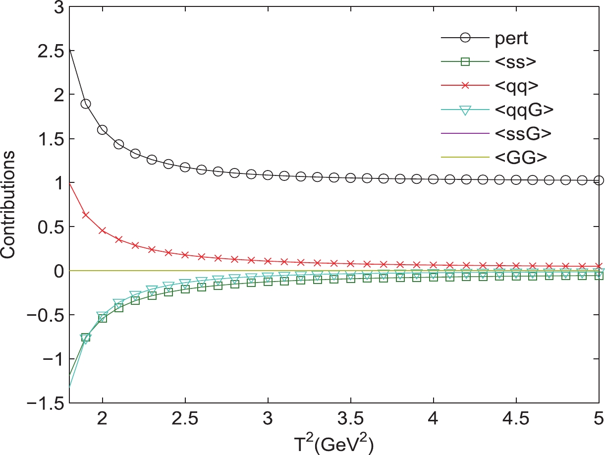
Figure 1. (color online) Contributions of different condensate terms for
$ \Xi_{b} $ (${3}/{2}^{+} $ ) of the excitation mode ($ L_{\rho},L_{\lambda})= $ $( 0,2 $ ), with variations in the Borel parameters$ T^{2} .$ After repeated adjustment and comparison, we finally determine the optimal energy scales μ, the Borel windows, the continuum threshold parameters
$ s_{0} $ , and the pole contributions, which are presented in Tables 1, 2. As an example, the results for$ 1D $ states with different excitation modes are shown explicitly in Figs. 2–25. Note that we plot the masses and pole residues with variations in the Borel parameters at much larger intervals than the Borel windows shown in Tables 1, 2. Additionally, the uncertainties of the masses and pole residues are marked as the upper and lower bounds in these figures. From Tables 1, 2, we observe that the pole contributions are about$ 40%–80% $ , and the pole dominance criterion is satisfied. However, we can observe that flat platforms appear in Figs. 2–25, and the uncertainties originating from the Borel parameters$ T^2 $ in the Borel window are small ($ \leq3 $ %). In other words, all of the criteria of QCD sum rules are satisfied, and it is reliable to extract the final results about the D-wave bottom baryons. Considering all uncertainties of the input parameters, we obtain the masses and pole residues of$ 1D $ and$ 2D $ states of$ \Lambda_{b} $ and$ \Xi_{b} $ baryons, which are also presentd in Tables 1, 2.$ \Xi_{b} (L_{\rho},l_{\lambda})$ 

$ J^{P} $ 

μ/GeV2 T2/GeV2 $ \sqrt{s_{0}}/{\rm GeV} $ 

M/GeV Refs. [15, 18]/GeV λ/(10−1 GeV5) pole $ \Xi_{b} $ (

$ 2,0 $ )

$ {5}/{2}^{+} $ (

$ 1 D$ )

$ 3.7 $ 

$ 3.8-4.2 $ 

$ 7.0\pm0.1 $ 

$ 6.43^{+0.10}_{-0.10} $ 

$ 1.59_{-0.18}^{+0.20} $ 

$49{\text{%} }-59{\text{%} }$ 

$ \Xi_{b} $ (

$ 2,0 $ )

$ {3}/{2}^{+} $ (

$ 1D $ )

$ 3.5 $ 

$ 3.9-4.3 $ 

$ 7.0\pm0.1 $ 

$ 6.42^{+0.09}_{-0.09} $ 

$ 4.64^{+0.60}_{-0.59} $ 

$ 47{\text{%} }-57{\text{%}}$ 

$ \Xi_{b} $ (

$ 0,2 $ )

$ {5}/{2}^{+} $ (

$ 1D $ )

$ 3.6 $ 

$ 4.3-4.7 $ 

$ 6.9\pm0.1 $ 

$ 6.36^{+0.11}_{-0.12} $ 

$ 6.333 $ [18]

$ 0.67^{+0.08}_{-0.07} $ 

$ 41{\text{%} }-56{\text{%}}$ 

$ \Xi_{b} $ (

$ 0,2 $ )

${3}/{2}^{+} $ (

$ 1D $ )

$ 3.6 $ 

$ 3.6-4.0 $ 

$ 6.9\pm0.1 $ 

$ 6.34^{+0.12}_{-0.11} $ 

$ 6.327 $ [18]

$ 2.98^{+0.38}_{-0.32} $ 

$ 41{\text{%} }-61{\text{%}}$ 

$ \Xi_{b} $ (

$ 1,1 $ )

$ {5}/{2}^{+} $ (

$ 1D $ )

$ 3.6 $ 

$ 4.2-4.6 $ 

$ 6.9\pm0.1 $ 

$ 6.41^{+0.09}_{-0.11} $ 

$ 0.80^{+0.11}_{-0.12} $ 

$ 42{\text{%} }-58{\text{%}}$ 

$ \Xi_{b} $ (

$ 1,1 $ )

$ {3}/{2}^{+} $ (

$ 1D $ )

$ 3.7 $ 

$ 3.8-4.2 $ 

$ 7.0\pm0.1 $ 

$ 6.41^{+0.09}_{-0.11} $ 

$ 2.82^{+0.30}_{-0.32} $ 

$ 47{\text{%} }-57{\text{%}}$ 

$ \Xi_{b} $ (

$ 2,0 $ )

${5}/{2}^{+}$ (

$ 2D$ )

$ 4.1 $ 

$ 3.9-4.3 $ 

$ 7.3\pm0.1 $ 

$ 6.77^{+0.12}_{-0.11} $ 

$ 2.46_{-0.19}^{+0.23} $ 

$ 65{\text{%} }-77{\text{%}}$ 

$ \Xi_{b} $ (

$ 2,0 $ )

${3}/{2}^{+}$ (

$ 2D$ )

$ 4.2 $ 

$ 3.9-4.3 $ 

$ 7.3\pm0.1 $ 

$ 6.73^{+0.09}_{-0.10} $ 

$ 7.13^{+0.55}_{-0.60} $ 

$ 66{\text{%} }-76{\text{%}}$ 

$ \Xi_{b} $ (

$ 0,2 $ )

${5}/{2}^{+}$ (

$ 2D$ )

$ 4.1 $ 

$ 4.3-4.7 $ 

$ 7.2\pm0.1 $ 

$ 6.69^{+0.13}_{-0.11} $ 

$ 6.696 $ [15]

$ 0.98^{+0.10}_{-0.12} $ 

$ 60{\text{%} }-68{\text{%}}$ 

$ \Xi_{b} $ (

$ 0,2 $ )

${3}/{2}^{+}$ (

$ 2D$ )

$ 4.1 $ 

$ 3.7-4.1 $ 

$ 7.2\pm0.1 $ 

$ 6.62^{+0.10}_{-0.13} $ 

$ 6.690 $ [15]

$ 4.29^{+0.42}_{-0.38} $ 

$ 53{\text{%} }-75{\text{%}}$ 

$ \Xi_{b} $ (

$ 1,1 $ )

${5}/{2}^{+}$ (

$ 2D $ )

$ 4.1 $ 

$ 4.2-4.6 $ 

$ 7.2\pm0.1 $ 

$ 6.72^{+0.11}_{-0.13} $ 

$ 1.19^{+0.13}_{-0.15} $ 

$ 57{\text{%} }-70{\text{%}}$ 

$ \Xi_{b} $ (

$ 1,1 $ )

$ {3}/{2}^{+} $ (

$ 2D $ )

$ 4.1 $ 

$ 3.8-4.2 $ 

$ 7.3\pm0.1 $ 

$ 6.79^{+0.12}_{-0.09} $ 

$ 3.53^{+0.35}_{-0.40} $ 

$ 65{\text{%} }-78{\text{%}}$ 

Table 1. Optimal energy scales μ, Borel parameters
$ T^{2} $ , continuum threshold parameters$ s_{0} $ , pole contributions (pole) and masses, and pole residues for the D-wave bottom baryon states$ \Xi_{b} $ , where the results of Ref. [15] are the quark-model predictions.$ \Lambda_{b} $ 

$ (L_{\rho},l_{\lambda}) $ 

$ J^{P} $ 

μ/GeV $ ^{2} $ 

$ T^{2} $ /GeV

$ ^{2} $ 

$ \sqrt{s_{0}} $ /GeV

M/GeV Ref. [9, 15]/GeV λ/( $ 10^{-1} $ GeV

$ ^{5} $ )

pole $ \Lambda_{b} $ (

$ 2,0 $ )

${5/}{2}^{+} $ (

$ 1 D$ )

$ 3.2 $ 

$ 3.5-3.9 $ 

$ 6.8\pm0.1 $ 

$ 6.28^{+0.10}_{-0.10} $ 

$ 0.96^{+0.10}_{-0.13} $ 

$ 42{\text{%} }-58{\text{%}}$ 

$ \Lambda_{b} $ (

$ 2,0 $ )

$ {3}/{2}^{+} $ (

$ 1D $ )

$ 3.2 $ 

$ 3.3-3.7 $ 

$ 6.7\pm0.1 $ 

$ 6.21^{+0.10}_{-0.10} $ 

$ 2.23^{+0.35}_{-0.33} $ 

$ 44{\text{%} }-56{\text{%}}$ 

$ \Lambda_{b} $ (

$ 0,2 $ )

$ {5}/{2}^{+} $ (

$ 1D $ )

$ 3.2 $ 

$ 3.7-4.1 $ 

$ 6.7\pm0.1 $ 

$ 6.15^{+0.13}_{-0.15} $ 

$ 6.153 $ [9]

$ 0.37^{+0.05}_{-0.04} $ 

$ 41{\text{%} }-56{\text{%}}$ 

$ \Lambda_{b} $ (

$ 0,2 $ )

$ {3}/{2}^{+} $ (

$ 1D $ )

$ 3.2 $ 

$ 3.4-3.8 $ 

$ 6.6\pm0.1 $ 

$ 6.13^{+0.10}_{-0.09} $ 

$ 6.146 $ [9]

$ 1.45^{+0.21}_{-0.22} $ 

$ 44{\text{%} }-59{\text{%}}$ 

$ \Lambda_{b} $ (

$ 1,1 $ )

$ {5}/{2}^{+} $ (

$ 1D $ )

$ 3.2 $ 

$ 3.9-4.3 $ 

$ 6.8\pm0.1 $ 

$ 6.29^{+0.08}_{-0.06} $ 

$ 0.54^{+0.08}_{-0.09} $ 

$ 45{\text{%} }-60{\text{%}}$ 

$ \Lambda_{b} $ (

$ 1,1 $ )

${3}/{2}^{+} $ (

$ 1 $ D)

$ 3.4 $ 

$ 3.5-3.9 $ 

$ 6.8\pm0.1 $ 

$ 6.30^{+0.08}_{-0.07} $ 

$ 1.77^{+0.31}_{-0.28} $ 

$ 42{\text{%} }-57{\text{%}}$ 

$ \Lambda_{b} $ (

$ 2,0 $ )

$ {5}/{2}^{+} $ (

$ 2D $ )

$ 3.9 $ 

$ 3.7-4.1 $ 

$ 7.1\pm0.1 $ 

$ 6.57^{+0.12}_{-0.11} $ 

$ 1.84^{+0.18}_{-0.20} $ 

$ 59{\text{%} }-73{\text{%}}$ 

$ \Lambda_{b} $ (

$ 2,0 $ )

${3}/{2}^{+}$ (

$ 2D $ )

$ 3.9 $ 

$ 3.6-4.0 $ 

$ 7.0\pm0.1 $ 

$ 6.50^{+0.11}_{-0.11} $ 

$ 4.65^{+0.42}_{-0.38} $ 

$ 56{\text{%} }-67{\text{%}}$ 

$ \Lambda_{b} $ (

$ 0,2 $ )

$ {5}/{2}^{+} $ (

$ 2D $ )

$ 3.8 $ 

$ 3.9-4.3 $ 

$ 7.0\pm0.1 $ 

$ 6.53^{+0.14}_{-0.14} $ 

$ 6.531 $ [15]

$ 0.83^{+0.08}_{-0.07} $ 

$ 61{\text{%} }-71{\text{%}}$ 

$ \Lambda_{b} $ (

$ 0,2 $ )

$ {3}/{2}^{+} $ (

$ 2 $ D)

$ 3.8 $ 

$ 3.6-4.0 $ 

$ 6.9\pm0.1 $ 

$ 6.47^{+0.09}_{-0.10} $ 

$ 6.526 $ [15]

$ 3.00^{+0.31}_{-0.30} $ 

$ 50{\text{%} }-65{\text{%}}$ 

$ \Lambda_{b} $ (

$ 1,1 $ )

${5}/{2}^{+} $ (

$ 2 D$ )

$ 3.9 $ 

$ 4.1-4.5 $ 

$ 7.1\pm0.1 $ 

$ 6.62^{+0.10}_{-0.08} $ 

$ 1.05^{+0.12}_{-0.13} $ 

$ 53{\text{%} }-66{\text{%}}$ 

$ \Lambda_{b} $ (

$ 1,1 $ )

$ {3}/{2}^{+} $ (

$ 2 D$ )

$ 3.9 $ 

$ 3.7-4.1 $ 

$ 7.1\pm0.1 $ 

$ 6.60^{+0.09}_{-0.09} $ 

$ 2.96^{+0.42}_{-0.39} $ 

$ 56{\text{%} }-72{\text{%}}$ 

Table 2. Optimal energy scales μ, Borel parameters
$ T^{2} $ , continuum threshold parameters$ s_{0} $ , pole contributions (pole) and masses, and pole residues for the D-wave bottom baryon states$ \Lambda_{b} $ , where the results of Ref. [15] are the quark-model predictions.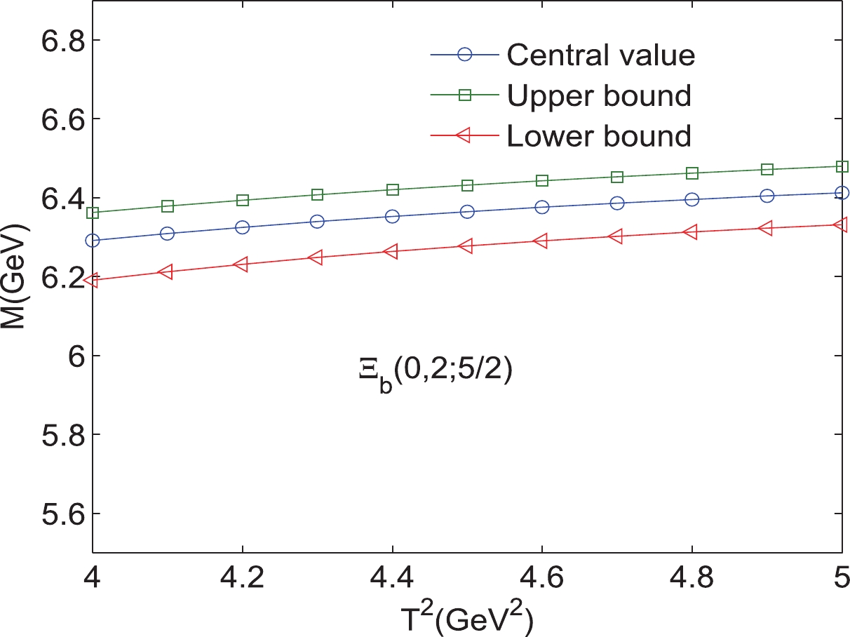
Figure 2. (color online) Mass of the bottom baryon state
$ \Xi_{b} $ (0,2,$ {5}/{2} $ ) with variations in the Borel parameters$ T^{2}. $ 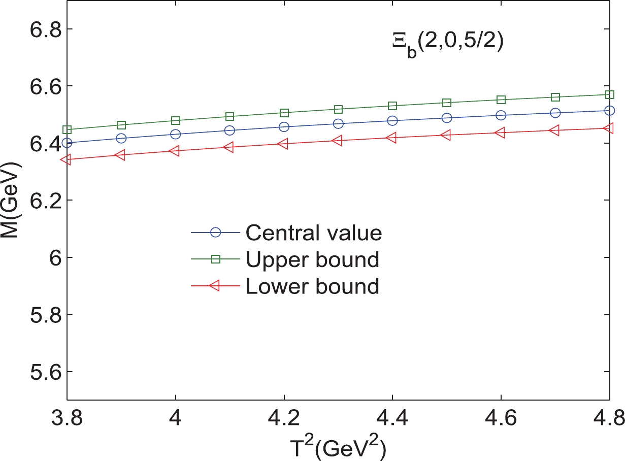
Figure 3. (color online) Mass of the bottom baryon state
$ \Xi_{b} $ (2,0,$ {5}/{2} $ ) with variations in the Borel parameters$ T^{2}. $ 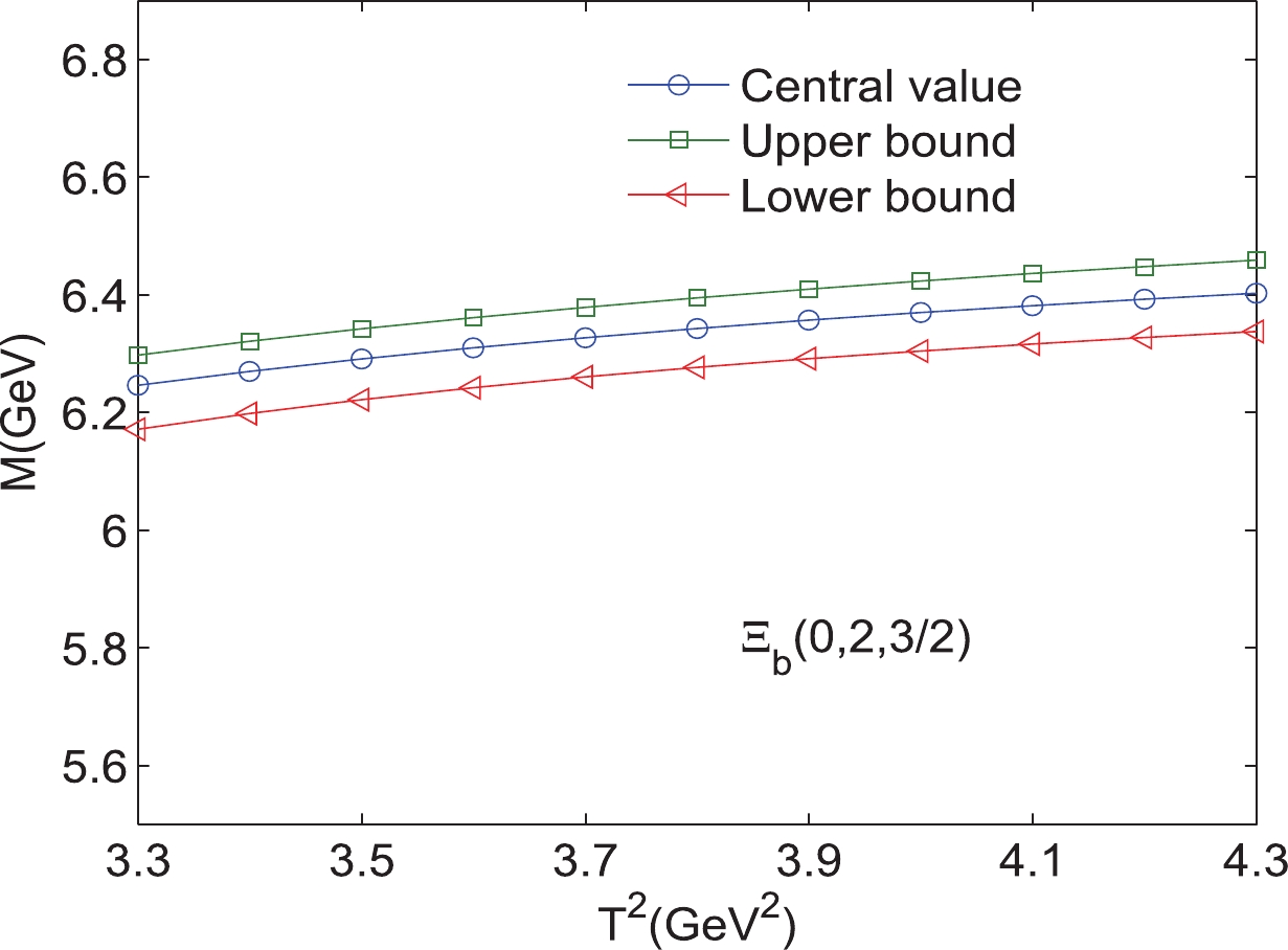
Figure 4. (color online) Mass of the bottom baryon state
$ \Xi_{b} $ (0,2,$ {3}/{2} $ ) with variations in the Borel parameters$ T^{2}. $ 
Figure 5. (color online) Mass of the bottom baryon state
$ \Xi_{b} $ (2,0,${3}/{2} $ ) with variations in the Borel parameters$ T^{2}. $ 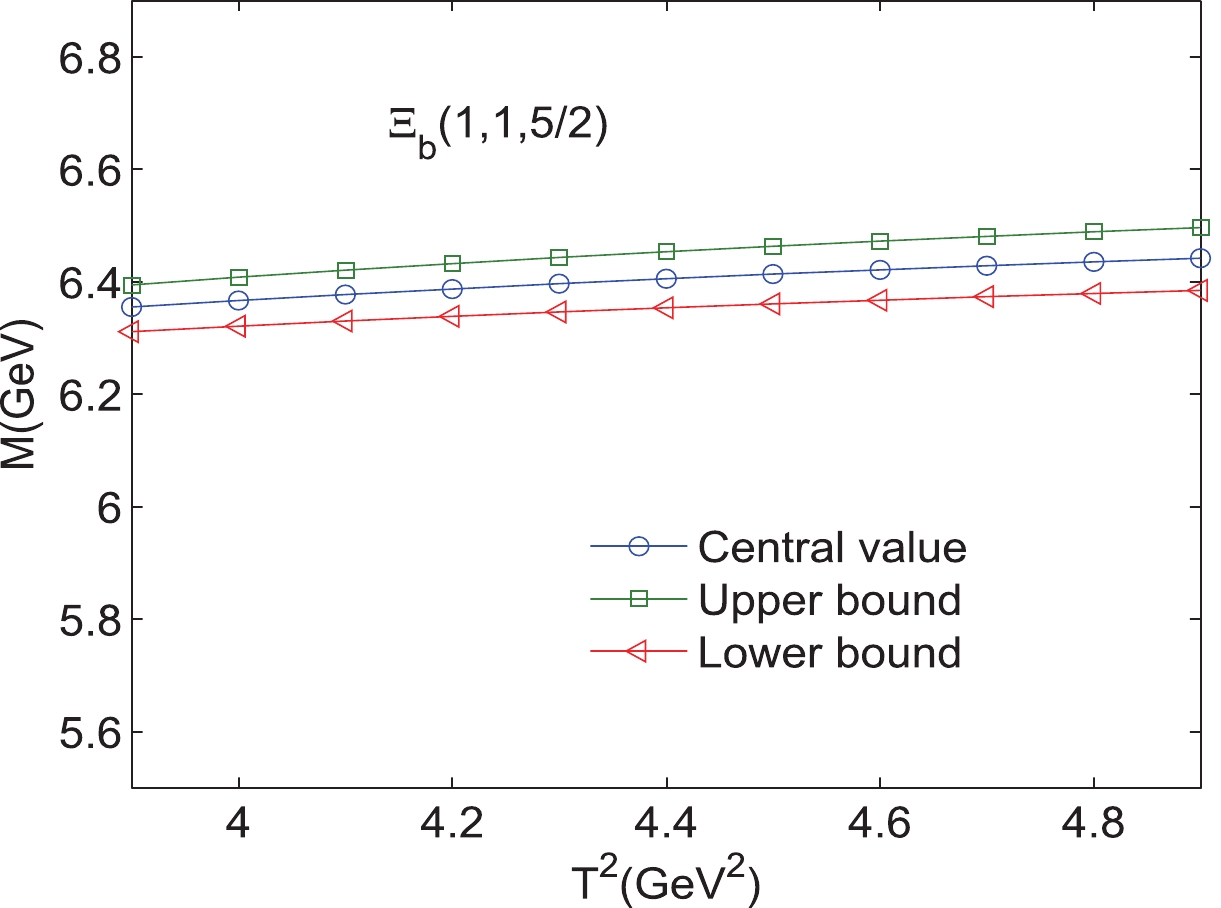
Figure 6. (color online) Mass of the bottom baryon state
$ \Xi_{b} $ (1,1,${5}/{2} $ ) with variations in the Borel parameters$ T^{2}. $ 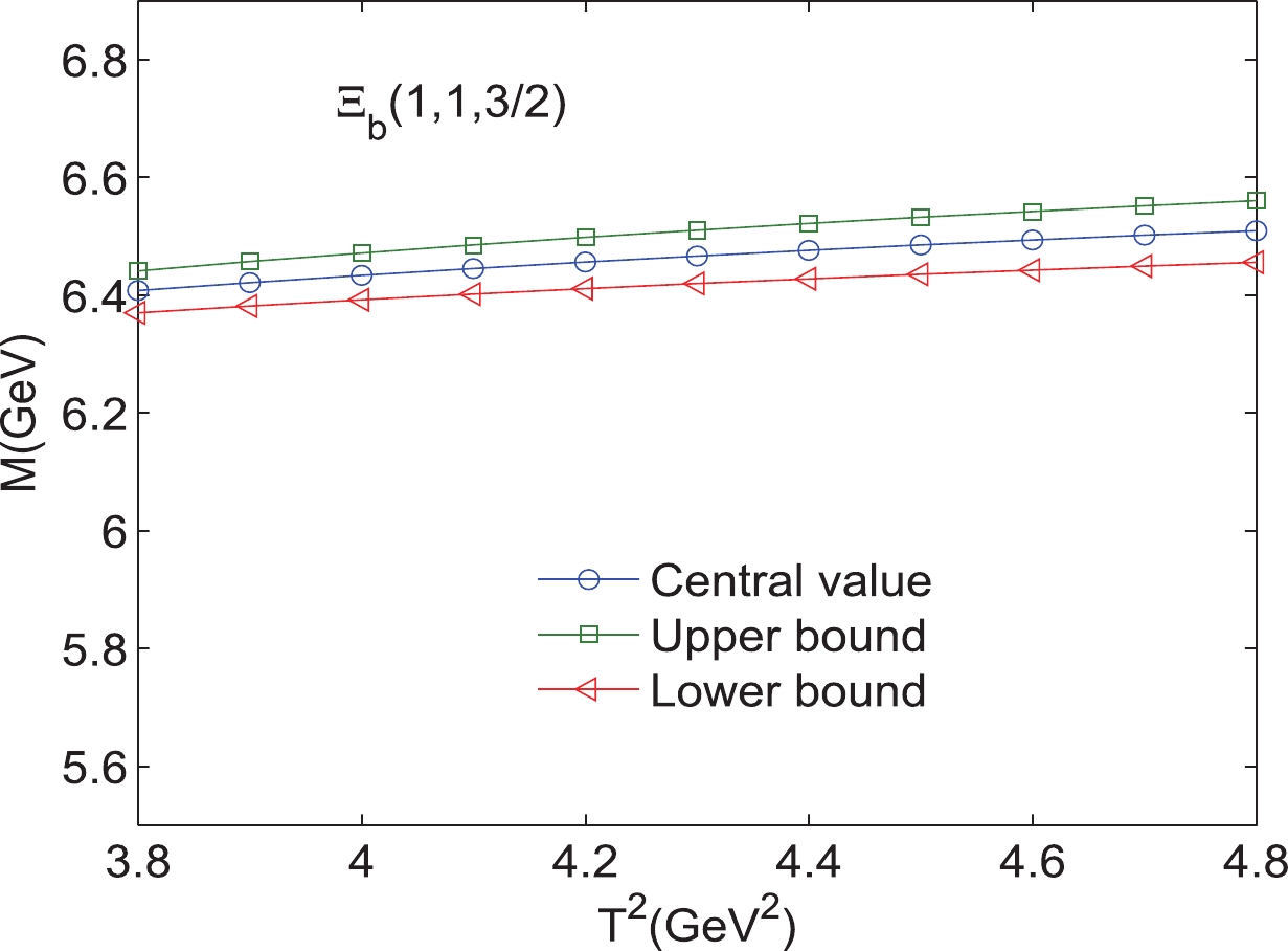
Figure 7. (color online) Mass of the bottom baryon state
$ \Xi_{b} $ (1,1,${3}/{2} $ ) with variations in the Borel parameters$ T^{2}. $ 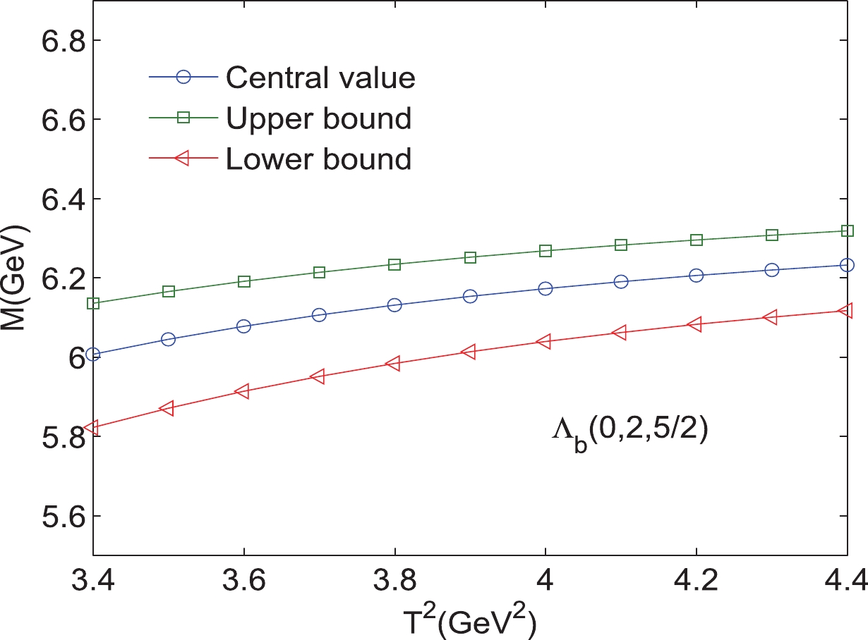
Figure 8. (color online) Mass of the bottom baryon state
$ \Lambda_{b} $ (0,2,$ {5}/{2} $ ) with variations in the Borel parameters$ T^{2}. $ 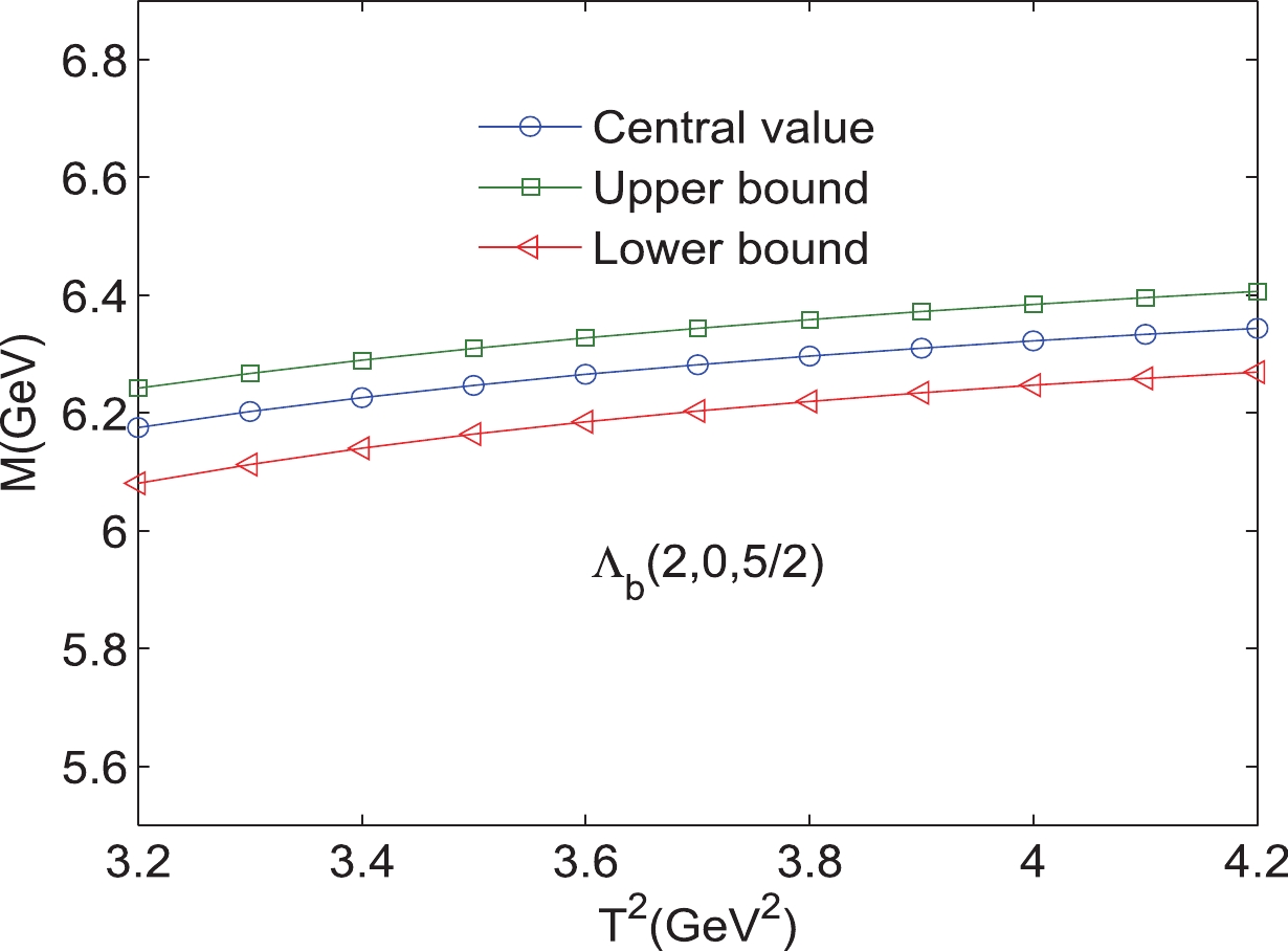
Figure 9. (color online) Mass of the bottom baryon state
$ \Lambda_{b} $ (2,0,$ {5}/{2} $ ) with variations in the Borel parameters$ T^{2}. $ 
Figure 10. (color online) Mass of the bottom baryon state
$ \Lambda_{b} $ (0,2,$ {3}/{2} $ ) with variations in the Borel parameters$ T^{2}. $ 
Figure 11. (color online) Mass of the bottom baryon state
$ \Lambda_{b} $ (2,0,$ {3}/{2} $ ) with variations in the Borel parameters$ T^{2}. $ 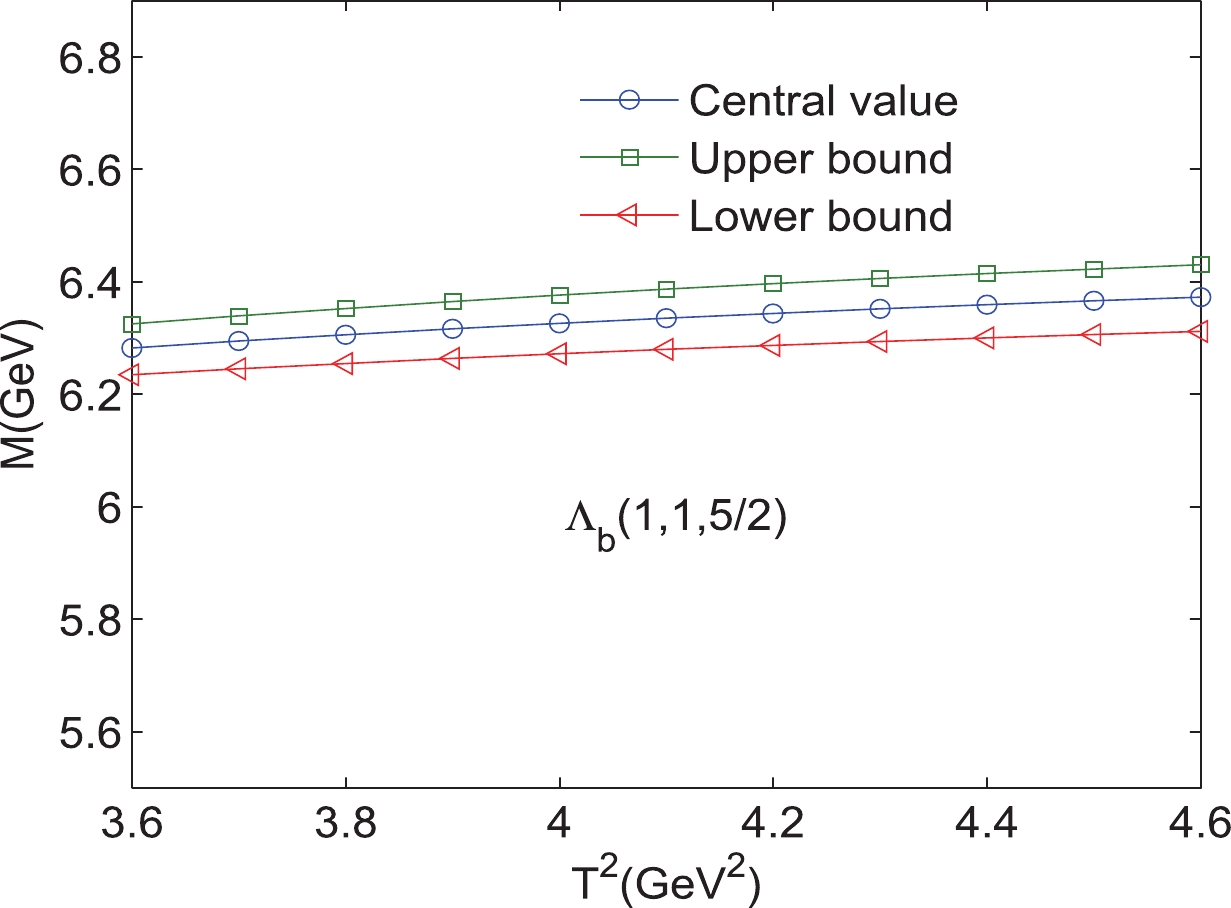
Figure 12. (color online) Mass of the bottom baryon state
$ \Lambda_{b} $ (1,1,$ {5}/{2} $ ) with variations in the Borel parameters$ T^{2}. $ 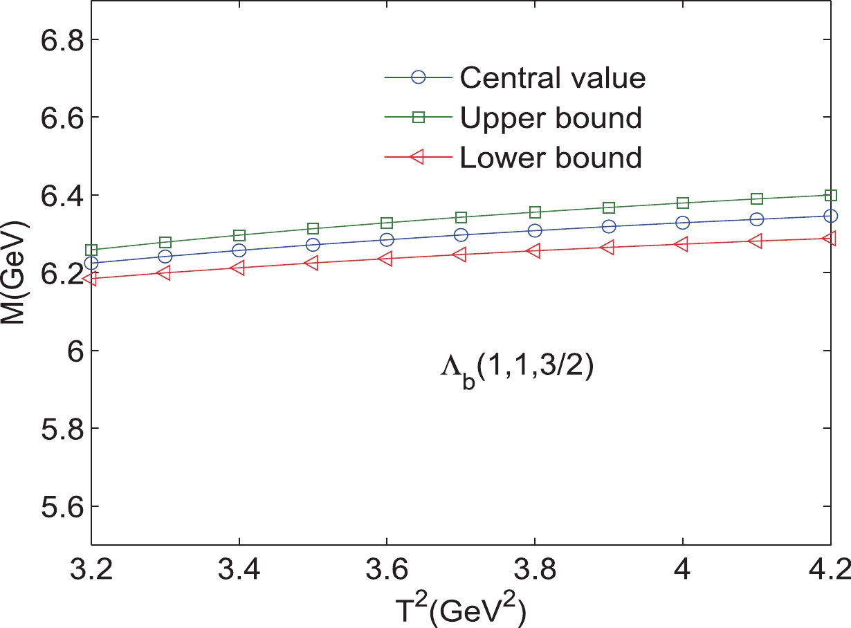
Figure 13. (color online) Mass of the bottom baryon state
$ \Lambda_{b} $ (1,1,$ {3}/{2} $ ) with variations in the Borel parameters$ T^{2}. $ 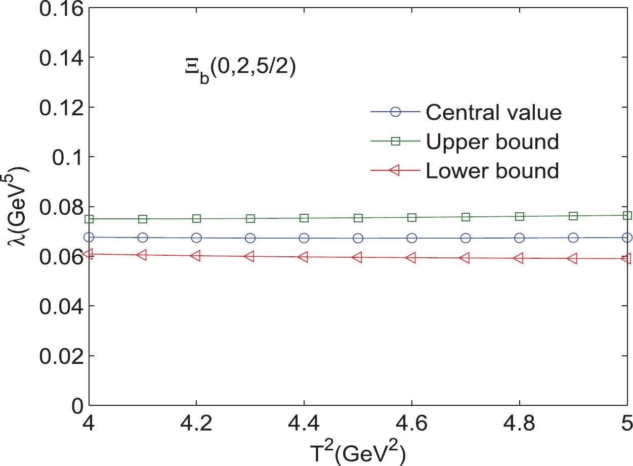
Figure 14. (color online) Pole residues of the bottom baryon state
$ \Xi_{b} $ (0,2,$ {5}/{2} $ ) with variations in the Borel parameters$ T^{2}. $ 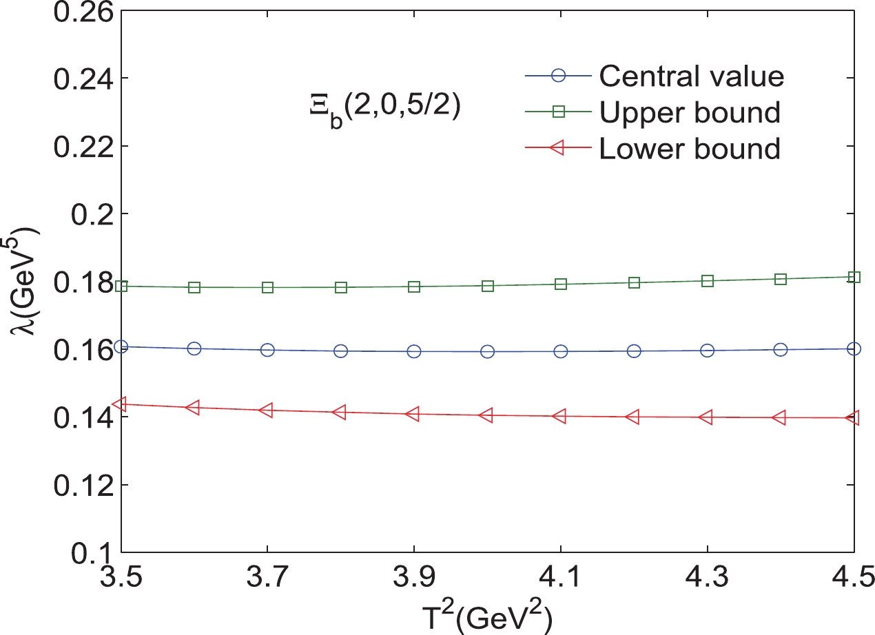
Figure 15. (color online) Pole residues of the bottom baryon state
$ \Xi_{b} $ (2,0,$ {5}/{2} $ ) with variations in the Borel parameters$ T^{2}. $ 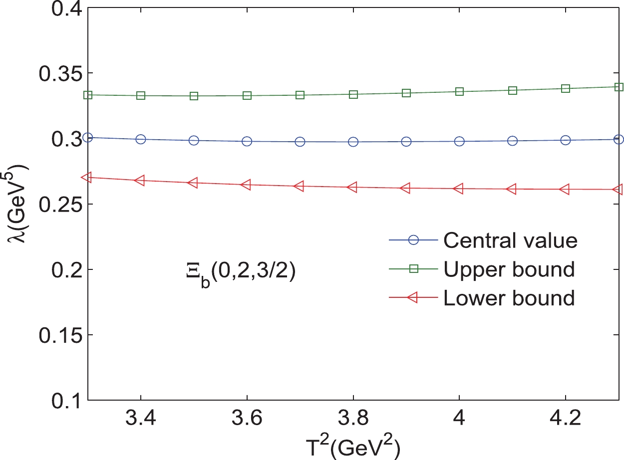
Figure 16. (color online) Pole residues of the bottom baryon state
$ \Xi_{b} $ (0,2,${3}/{2} $ ) with variations in the Borel parameters$ T^{2}. $ 
Figure 17. (color online) Pole residues of the bottom baryon state
$ \Xi_{b} $ (2,0,$ {3}/{2} $ ) with variations in the Borel parameters$ T^{2}. $ 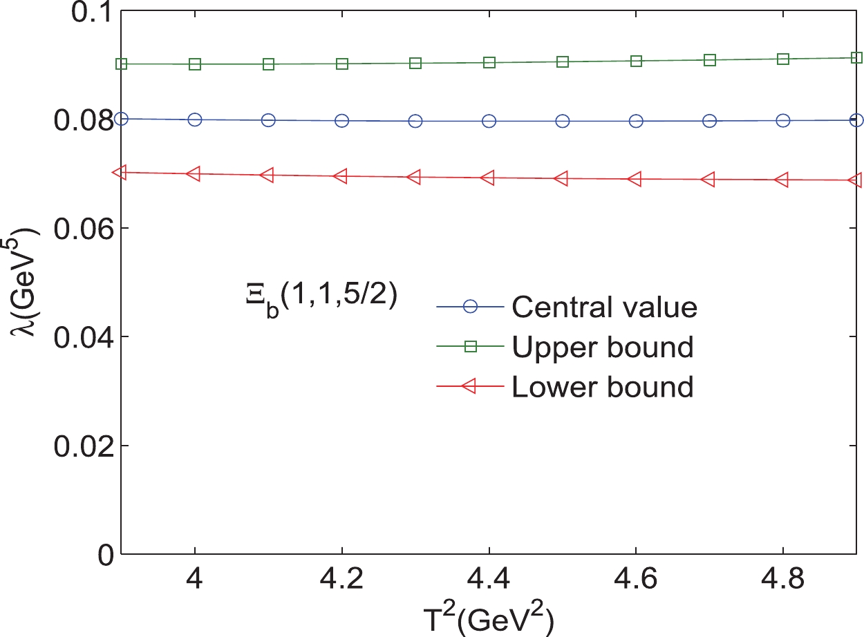
Figure 18. (color online) Pole residues of the bottom baryon state
$ \Xi_{b} $ (1,1,$ {5}/{2} $ ) with variations in the Borel parameters$ T^{2}. $ 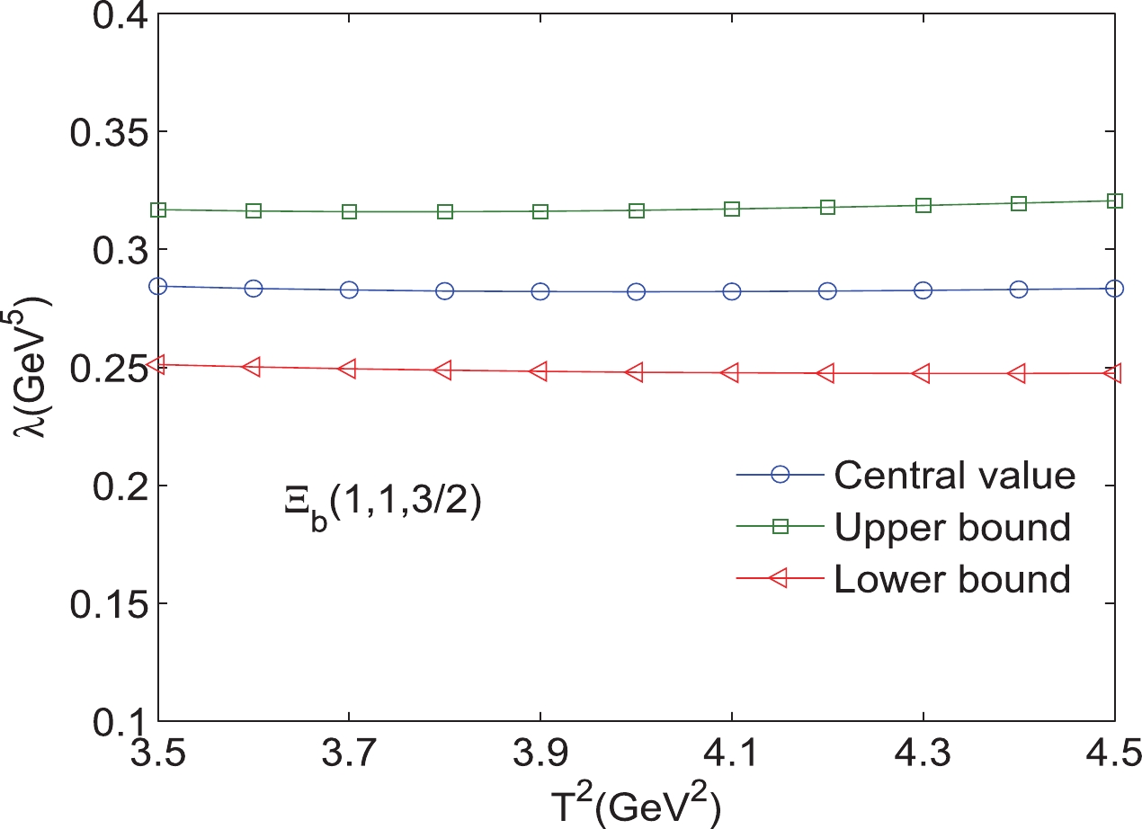
Figure 19. (color online) Pole residues of the bottom baryon state
$ \Xi_{b} $ (1,1,$ {3}/{2} $ ) with variations in the Borel parameters$ T^{2}. $ 
Figure 20. (color online) Pole residues of the bottom baryon state
$ \Lambda_{b} $ (0,2,$ {5}/{2} $ ) with variations in the Borel parameters$ T^{2}. $ 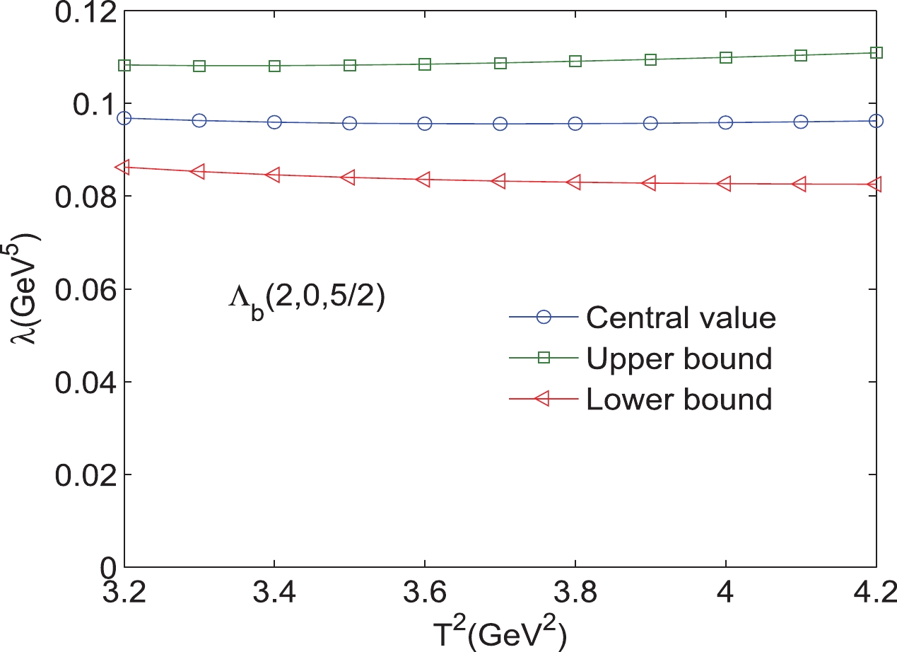
Figure 21. (color online) Pole residues of the bottom baryon state
$ \Lambda_{b} $ (2,0,${5}/{2} $ ) with variations in the Borel parameters$ T^{2}. $ 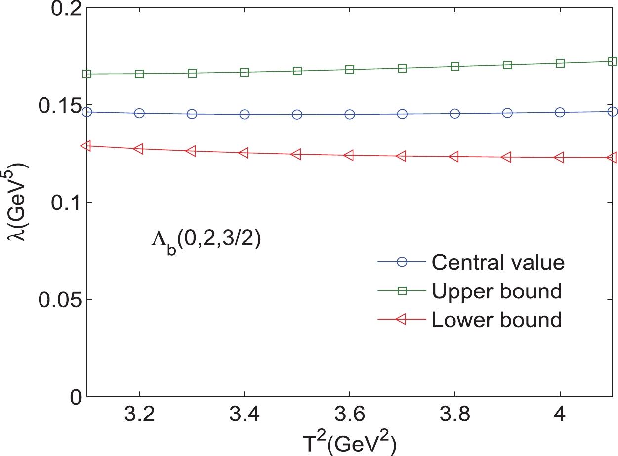
Figure 22. (color online) Pole residues of the bottom baryon state
$ \Lambda_{b} $ (0,2,$ {3}/{2} $ ) with variations in the Borel parameters$ T^{2}. $ 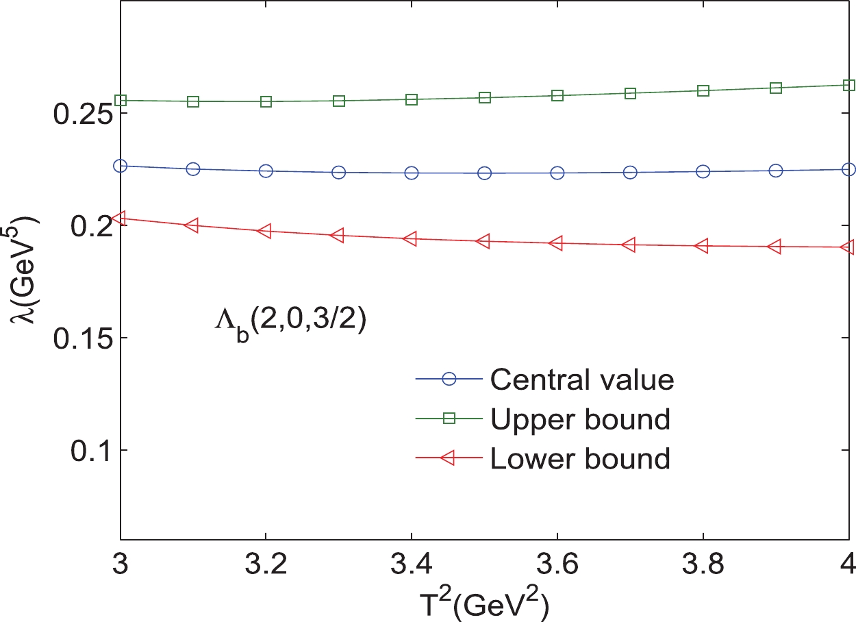
Figure 23. (color online) Pole residues of the bottom baryon state
$ \Lambda_{b} $ (2,0,$ {3}/{2} $ ) with variations in the Borel parameters$ T^{2}. $ 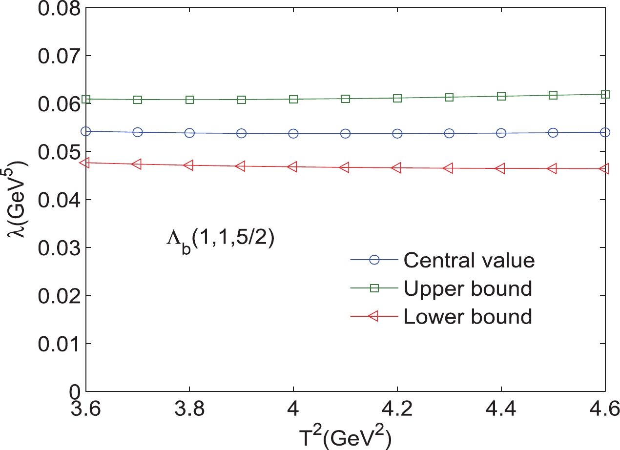
Figure 24. (color online) Pole residues of the bottom baryon state
$ \Lambda_{b} $ (1,1,${5}/{2} $ ) with variations in the Borel parameters$ T^{2}. $ 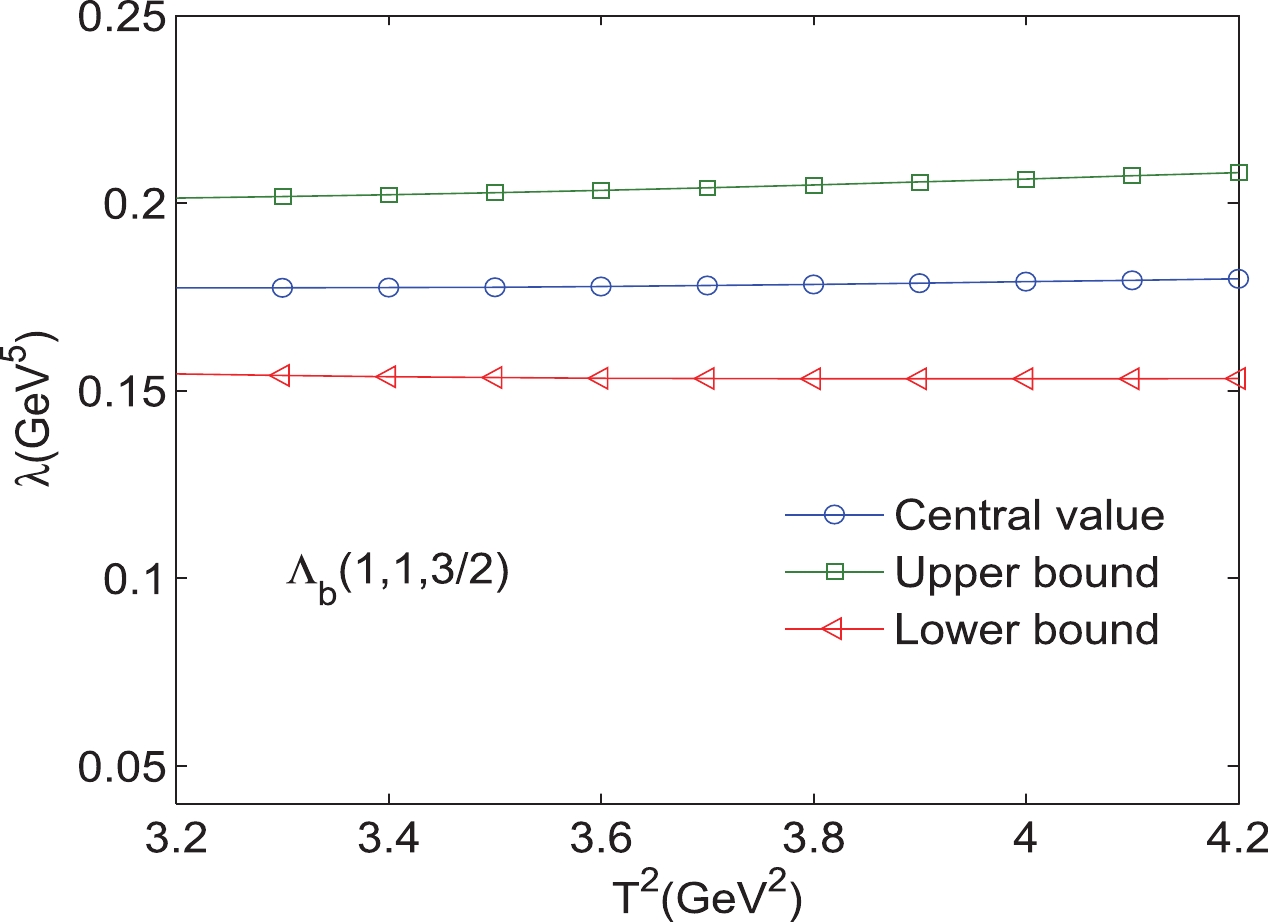
Figure 25. (color online) Pole residues of the bottom baryon state
$ \Lambda_{b} $ (1,1,$ {3}/{2} $ ) with variations in the Borel parameters$ T^{2}. $ The LHCb collaboration observed two structures with the masses of
$ m_{\Lambda_{b}}(6146)^{0}=6146.17\pm0.33\pm0.22\pm0.16 $ MeV and$ m_{\Lambda_{b}}(6152)^{0}=6152.51\pm0.26\pm0.22\pm0.16 $ MeV and suggested their possible interpretation as a doublet of the$ \Lambda_{b}(1D) $ state. The quark-model predictions from different collaborations for the masses of this doublet ($ {3}/{2}^{+} $ ,$ {5}/{2}^{+} $ ) were ($ 6.145 $ ,$ 6.165 $ GeV) [14], ($ 6.190 $ ,$ 6.196 $ GeV) [15], ($ 6.181 $ ,$ 6.183 $ GeV) [16] and ($ 6.147 $ ,$ 6.153 $ GeV) [17]. Our predictions for this doublet with the excitation mode ($ L_{\rho},L_{\lambda}– $ $ (0,2 $ ) are$ m_{\Lambda_{b}}^{{3}/{2}^{+}}=6.13^{+0.10}_{-0.09} $ GeV and$ m_{\Lambda_{b}}^{{5}/{2}^{+}}=6.15^{+0.13}_{-0.15} $ GeV, respectively. This result is consistent with experimental data [9] and quark-model predictions [14, 17], which supports assigning$ \Lambda_{b}(6146) $ and$ \Lambda_{b}(6152) $ as the$ 1D \Lambda_{b} $ doublet with the quantum numbers ($ L_{\rho},L_{\lambda})=( $ $ 0,2 $ ) and$ J^{p}= $ $ {3} {2}^{+} $ ,${5}/{2}^{+} $ .To date, the 1S, 1P, and 1D
$ \Lambda_{b} $ baryons have been established, but as for the$ \Xi_{b} $ sector, only the ground state$ \Xi_{b}(5797) $ has been confirmed [89]. In particular, for radially excited$ \Xi_{b} $ and$ \Lambda_{b} $ states, fewer experimental results have been reported [3]. In Ref. [15], the mass spectra of$ \Xi_{b} $ baryons were calculated in the heavy-quark-light-diquark picture in the framework of the QCD-motivated relativistic quark model. In Refs. [6, 10], the masses and strong decay properties of$ 1D \Xi_{b} $ baryons with$ J^{p}= $ ${3}/{2}^{+} $ and$ {5}/{2}^{+} $ were studied using the quark and$ ^{3}P_{0} $ models. These calculations with the quark model were performed by considering bottom baryons as the excitation mode ($ L_{\rho},L_{\lambda})= $ $( 0,2 $ ). Their predicted masses for the$ 1D \Xi_{b} $ doublet were ($ 6366 $ MeV,$ 6373 $ MeV) in Ref. [15] and ($ 6327 $ MeV,$ 6330 $ MeV) in Refs. [6, 10], respectively. Table 1 shows that the QCD sum rule predictions for the masses of this doublet with excitation mode ($ L_{\rho},L_{\lambda})= $ $ (0,2 $ ) are$ m_{{3}/{2}^{+}}=6.34^{+0.12}_{-0.11} $ GeV and$ m_{{5}/{2}^{+}}=6.36^{+0.11}_{-0.12} $ GeV, which are consistent with experiments [18] and the predictions in Refs. [6, 10]. Thus, it is reasonable to describe the$ \Xi_{b}(6327) $ and$ \Xi_{b}(6333) $ baryons as the$ 1D $ ($ \Xi_{b} $ ) doublet with the excited mode ($ L_{\rho},L_{\lambda})= $ $ (0,2 $ ) and quantum numbers$ J^{p}= $ $ {3}/{2}^{+} $ and$ {5}/{2}^{+} $ . For the$ 2D \Lambda_{b} $ and$ \Xi_{b} $ doublets, their masses with$ \lambda- $ mode were predicted as ($ 6526 $ MeV,$ 6531 $ MeV) and ($ 6690 $ MeV,$ 6696 $ MeV) in Ref. [15], which is roughly compatible with our results ($ 6.47^{+0.09}_{-0.10} $ GeV,$ 6.53^{+0.14}_{-0.14} $ GeV) and ($ 6.62^{+0.10}_{-0.13} $ GeV,$ 6.69^{+0.13}_{-0.11} $ GeV). From Tables 1–2, we also observe that for either the$ 1D $ or$ 2D $ state, the prediction for the mass of the orbital excitation mode ($ L_{\rho},L_{\lambda})= $ $ (0,2 $ ) is slightly lower than those of the other excitation modes. Except for the$ 1D \Xi_{b} $ states, the predicted mass for the excitation mode ($ L_{\rho},L_{\lambda})= $ $ (1,1 $ ) is slightly higher than the others.Finally, we would like to note that in addition to masses, decay and production properties are useful for revealing the inner structure of heavy baryons. The predicted pole residues for the D-wave
$ \Xi_{b} $ and$ \Lambda_{b} $ baryons in this paper will be useful parameters in studying the strong decay properties in the future. With the operation of the LHCb, we expect these excited$ \Xi_{b} $ and$ \Lambda_{b} $ baryons to be observed in the near future. -
In summary, theoretical and experimental physicists have achieved significant progress in the field of single bottom baryons such as
$ \Lambda_{b}(6072) $ [3, 4],$ \Lambda_{b}(6146) $ [10–13],$ \Lambda_{b}(6152) $ [10–13],$ \Xi_{b}(6227) $ [5–7],$ \Xi_{b}(6100) $ [8],$ \Xi_{b}(6327) $ [10, 18], and$ \Xi_{b}(6333) $ [10, 18]. Stimulated by the observations of these new bottom states, we systematically study the$ 1D $ and$ 2D $ $ \Lambda_{b} $ and$ \Xi_{b} $ baryons using the method of QCD sum rules. According to the heavy quark effective theory, we categorize the D-wave bottom baryons into three types, which are denoted by their orbital excitation modes:$ (L_{\rho},L_{\lambda})=(0,2) $ ,$ (2,0) $ , and$ (1,1) $ . According to these excitation modes, we construct three types of interpolating currents to study the$ 1D $ and$ 2D $ bottom baryons with spin-parity$ J^{p}={3}/{2}^{+} $ and$ {5}/{2}^{+} $ . In our calculations, we successfully separate the contributions of the positive and negative states, which causes the QCD sum rules to refrain from the contamination of the bottom baryon states with negative parity. We perform the OPE up to the vacuum condensates of dimension$ 10 $ to warrant the reliability of the final results. Our predictions favor assigning$ \Lambda_{b}(6146) $ and$ \Lambda_{b}(6152) $ as a$ 1D \Lambda_{b} $ doublet with quantum numbers of$ (L_{\rho},L_{\lambda})=(0,2) $ and$ J^{P}= $ ($ {3}/{2}^{+} $ ,$ {5}/{2}^{+} $ ), respectively. This conclusion is consistent with experiments and with those of other collaborations [9, 14, 17]. As for the$ \Xi_{b} $ ($ 1D $ ) states, we predict the masses of the excitation mode$ (L_{\rho},L_{\lambda})=(0,2) $ as$ m_{{3}/{2}^{+}}=6.34^{+0.12}_{-0.11} $ GeV and$ m_{{5}/{2}^{+}}=6.36^{+0.11}_{-0.12} $ GeV. This result is compatible with the experimental data [18] as well as the quark-model predictions [6, 10]. Thus, these two states can be interpreted as the$ \Xi_{b} $ ($ 1D $ ) doublet with the quantum numbers$ (L_{\rho},L_{\lambda})=(0,2) $ and$ J^{P}= $ $ {3}/{2}^{+} $ ,$ {5}/{2}^{+} $ , respectively. Finally, our results show that the prediction for the mass of the excitation mode$ (L_{\rho},L_{\lambda})=(0,2) $ is the smallest in these three excitation modes, and the mass of$ (L_{\rho},L_{\lambda})=(1,1) $ is the largest, except for the$ 1D \Xi_{b} $ state. The pole residues predicted in this paper are useful parameters in studying the strong decay properties of the$ 1D $ and$ 2D \Xi_{b} $ and$ \Lambda_{b} $ states. -
$ \begin{aligned}[b] \rho^{0,\Xi_{b}}_{{5}/{2},2,0}(s)=&\int^{1}_{{m^{2}_{b}}/{s}}\Bigg\{\frac{1}{69120\pi^{4}}\big(132 - 494 x + 665 x^2 - 360 x^3 + 50 x^4 - 2 x^5 + 9 x^6\big)\times\Bigg(s-\frac{m_{b}^{2}}{x}\Bigg)^{4}+\frac{m_{s}(5\langle \overline{s}s\rangle-2\langle \overline{q}q\rangle)}{96\pi^{2}}\\ &\times\big(x^2 - 2 x^3 + x^4\big)\times\Bigg(s-\frac{m_{b}^{2}}{x}\Bigg)^{2} -\frac{m_{s}\langle \overline{q}g_{s}\sigma Gq\rangle}{36\pi^{2}}\times\big(4 - 7 x +3 x^2\big)\times\Bigg(s-\frac{m_{b}^{2}}{x}\Bigg) +\frac{m_{s}\langle \overline{s}g_{s}\sigma Gs\rangle}{216\pi^{2}} \\ &\times\big(31 - 58 x + 27 x^2\big)\times\Bigg(s-\frac{m_{b}^{2}}{x}\Bigg) +\frac{1}{34560\pi^{2}}\langle\frac{\alpha_{s}GG}{\pi}\rangle\times\big(665 + 132/x^2 - 494/x - 360 x + 50 x^2 - 2 x^3 + 9 x^4\big)\\ &\times\Bigg(s-\frac{m_{b}^{2}}{x}\Bigg)^{2} +\frac{1}{6192\pi^{2}}\langle\frac{\alpha_{s}GG}{\pi}\rangle\times\big(46 - 72 x + 15 x^2 + 2 x^3 + 9 x^4\big)\times\Bigg(s-\frac{m_{b}^{2}}{x}\Bigg)^{2}\Bigg\}{\rm d}x\\ & +\frac{\langle \overline{q}g_{s}\sigma Gq\rangle\langle \overline{s}g_{s}\sigma Gs\rangle}{72}\delta\big(s-m_{b}^{2}\big), \end{aligned} \tag{A1}$

$ \begin{aligned}[b] \rho^{1,\Xi_{b}}_{{5}/{2},2,0}(s)=&\int^{1}_{{m^{2}_{b}}/{s}}\Bigg\{\frac{1}{69120\pi^{4}}\big(128 x - 457 x^2 + 575 x^3 - 290 x^4 + 70 x^5 - 53 x^6 + 27 x^7\big)\times\Bigg(s-\frac{m_{b}^{2}}{x}\Bigg)^{4}-\frac{m_{s}(5\langle \overline{s}s\rangle-2\langle \overline{q}q\rangle)}{288\pi^{2}}\\ &\times\big(x^2 - 11 x^3 + 19 x^4 - 9 x^5\big)\times\Bigg(s-\frac{m_{b}^{2}}{x}\Bigg)^{2} +\frac{m_{s}\langle \overline{q}g_{s}\sigma Gq\rangle}{72\pi^{2}}\times\big(x - 18 x^2 + 35 x^3 - 18 x^4\big)\times\Bigg(s-\frac{m_{b}^{2}}{x}\Bigg) \\ & -\frac{m_{s}\langle \overline{s}g_{s}\sigma Gs\rangle}{216\pi^{2}}\times\big(4 x - 74 x^2 + 151 x^3 - 81 x^4\big)\times\Bigg(s-\frac{m_{b}^{2}}{x}\Bigg) +\frac{1}{6192\pi^{2}}\langle\frac{\alpha_{s}GG}{\pi}\rangle\\ &\times\big(40 x - 57 x^2 + 21 x^3 - 31 x^4 + 27 x^5\big)\times\Bigg(s-\frac{m_{b}^{2}}{x}\Bigg)^{2} -\frac{m_{b}^{2}}{51840\pi^{2}}\langle\frac{\alpha_{s}GG}{\pi}\rangle \times\big(575 + 128/x^2 - 457/ x \\ &- 290 x + 70 x^2 - 53 x^3 + 27 x^4\big)\times\Bigg(s-\frac{m_{b}^{2}}{x}\Bigg)\Bigg\}{\rm d}x +\frac{5\langle \overline{q}g_{s}\sigma Gq\rangle\langle \overline{s}g_{s}\sigma Gs\rangle}{432}\delta\big(s-m_{b}^{2}\big), \end{aligned} \tag{A2}$

$ \begin{aligned}[b] \rho^{0,\Xi_{b}}_{{5}/{2},0,2}(s)=&\int^{1}_{{m^{2}_{b}}/{s}}\Bigg\{-\frac{1}{4608\pi^{4}}\big(2 x - 11 x^2 + 24 x^3 - 26 x^4 + 14 x^5 - 3 x^6\big)\times\Bigg(s-\frac{m_{b}^{2}}{x}\Bigg)^{4}+\frac{m_{s}(\langle \overline{s}s\rangle-2\langle \overline{q}q\rangle)}{96\pi^{2}}\\ &\times\big(x^2 - 2 x^3 + x^4\big)\times\Bigg(s-\frac{m_{b}^{2}}{x}\Bigg)^{2} +\frac{m_{b}^{2}}{3456\pi^{2}}\langle\frac{\alpha_{s}GG}{\pi}\rangle\times\big(24 + 2/x^2 - 11/x - 26 x + 14 x^2 - 3 x^3\big)\times\Bigg(s-\frac{m_{b}^{2}}{x}\Bigg) \\ & +\frac{1}{2304\pi^{2}}\langle\frac{\alpha_{s}GG}{\pi}\rangle\times\big(11 - 2/x - 24 x + 26 x^2 - 14 x^3 + 3 x^4\big)\times\Bigg(s-\frac{m_{b}^{2}}{x}\Bigg)^{2} +\frac{1}{768\pi^{2}}\langle\frac{\alpha_{s}GG}{\pi}\rangle\\ &\times\big(x^2 - 2 x^3 + x^4\big)\times\Bigg(s-\frac{m_{b}^{2}}{x}\Bigg)^{2} \Bigg\}{\rm d}x +\frac{\langle \overline{q}g_{s}\sigma Gq\rangle\langle \overline{s}g_{s}\sigma Gs\rangle}{72}\delta\big(s-m_{b}^{2}\big), \end{aligned} \tag{A3}$

$ \begin{aligned}[b] \rho^{1,\Xi_{b}}_{{5}/{2},0,2}(s)=&\int^{1}_{{m^{2}_{b}}/{s}}\Bigg\{\frac{1}{4608\pi^{4}}\big(x^2 + 5 x^3 - 30 x^4 + 50 x^5 - 35 x^6 + 9 x^7\big)\times\Bigg(s-\frac{m_{b}^{2}}{x}\Bigg)^{4}-\frac{m_{s}(\langle \overline{s}s\rangle-2\langle \overline{q}q\rangle)}{288\pi^{2}}\times\big(x^2 - 11 x^3 + 19 x^4 - 9 x^5\big)\\ &\times\Bigg(s-\frac{m_{b}^{2}}{x}\Bigg)^{2} -\frac{m_{b}^{2}}{3456\pi^{2}}\langle\frac{\alpha_{s}GG}{\pi}\rangle\times\big(5 + 1/x - 30 x + 50 x^2 - 35 x^3 + 9 x^4\big)\times\Bigg(s-\frac{m_{b}^{2}}{x}\Bigg) -\frac{1}{2304\pi^{2}}\langle\frac{\alpha_{s}GG}{\pi}\rangle\\ &\times\big(x^2 - 11 x^3 + 19 x^4 - 9 x^5\big)\times\Bigg(s-\frac{m_{b}^{2}}{x}\Bigg)^{2} \Bigg\}{\rm d}x +\frac{5\langle \overline{q}g_{s}\sigma Gq\rangle\langle \overline{s}g_{s}\sigma Gs\rangle}{432}\delta\big(s-m_{b}^{2}\big), \end{aligned} \tag{A4}$

$ \begin{aligned}[b] \rho^{0,\Xi_{b}}_{{5}/{2},1,1}(s)=&\int^{1}_{{m^{2}_{b}}/{s}}\Bigg\{-\frac{1}{13824\pi^{4}}\big(3 - 20 x + 47 x^2 - 48 x^3 + 17 x^4 + 4 x^5 - 3 x^6\big)\times\Bigg(s-\frac{m_{b}^{2}}{x}\Bigg)^{4}+\frac{m_{s}(3\langle \overline{s}s\rangle-2\langle \overline{q}q\rangle)}{96\pi^{2}}\times\big(x^2 - 2 x^3 + x^4\big)\\ &\times\Bigg(s-\frac{m_{b}^{2}}{x}\Bigg)^{2} -\frac{m_{s}\langle \overline{q}g_{s}\sigma Gq\rangle}{48\pi^{2}}\times\big(x - 3 x^2 + 2 x^3\big)\times\Bigg(s-\frac{m_{b}^{2}}{x}\Bigg) +\frac{5m_{s}\langle \overline{s}g_{s}\sigma Gs\rangle}{432\pi^{2}}\times\big(x - 4 x^2 + 3 x^3\big)\\ &\times\Bigg(s-\frac{m_{b}^{2}}{x}\Bigg) -\frac{m_{b}^{2}}{10368\pi^{2}}\langle\frac{\alpha_{s}GG}{\pi}\rangle\times\big(48 - 3/x^3 + 20/x^2 - 47/x - 17 x - 4 x^2 + 3 x^3\big)\times\Bigg(s-\frac{m_{b}^{2}}{x}\Bigg) \\ & -\frac{1}{6192\pi^{2}}\langle\frac{\alpha_{s}GG}{\pi}\rangle\times\big(47 + 3/x^2 - 20/x - 48 x + 17 x^2 + 4 x^3 - 3 x^4\big)\times\Bigg(s-\frac{m_{b}^{2}}{x}\Bigg)^{2} \\ & -\frac{1}{4608\pi^{2}}\langle\frac{\alpha_{s}GG}{\pi}\rangle\times\big(1 - 12 x + 15 x^2 + 2 x^3 - 6 x^4\big)\times\Bigg(s-\frac{m_{b}^{2}}{x}\Bigg)^{2}\Bigg\}{\rm d}x, \end{aligned} \tag{A5}$

$ \begin{aligned}[b] \rho^{1,\Xi_{b}}_{\frac{5}{2},1,1}(s)=&\int^{1}_{\frac{m^{2}_{b}}{s}}\Bigg\{\frac{1}{13824\pi^{4}}\big(2 x + 6 x^2 - 35 x^3 + 40 x^4 - 22 x^6 + 9 x^7\big)\times\Bigg(s-\frac{m_{b}^{2}}{x}\Bigg)^{4}-\frac{m_{s}(3\langle \overline{s}s\rangle-2\langle \overline{q}q\rangle)}{288\pi^{2}}\times\big(x^2 - 11 x^3 + 19 x^4 - 9 x^5\big)\\ &\times\Bigg(s-\frac{m_{b}^{2}}{x}\Bigg)^{2} +\frac{m_{s}\langle \overline{q}g_{s}\sigma Gq\rangle}{288\pi^{2}}\times\big(x - 22 x^2 + 57 x^3 - 36 x^4\big)\times\Bigg(s-\frac{m_{b}^{2}}{x}\Bigg) -\frac{m_{s}\langle \overline{s}g_{s}\sigma Gs\rangle}{432\pi^{2}}\times\big(x - 24 x^2 + 68 x^3\\ & - 45 x^4\big)\times\Bigg(s-\frac{m_{b}^{2}}{x}\Bigg) +\frac{m_{b}^{2}}{10368\pi^{2}}\langle\frac{\alpha_{s}GG}{\pi}\rangle\times\big(35 - 2/x^2 - 6/x - 40 x + 22 x^3 - 9 x^4\big)\times\Bigg(s-\frac{m_{b}^{2}}{x}\Bigg) \\ &+\frac{1}{4608\pi^{2}}\langle\frac{\alpha_{s}GG}{\pi}\rangle\times\big(x^2 + 16 x^3 - 35 x^4 + 18 x^5\big)\times\big(s-\frac{m_{b}^{2}}{x}\big)^{2}\Bigg\}{rm d}x \end{aligned} \tag{A6}$

$ \begin{aligned}[b] \rho^{0,\Xi_{b}}_{{3}/{2},2,0}(s)=&\int^{1}_{{m^{2}_{b}}/{s}}\Bigg\{\frac{1}{3072\pi^{4}}\big(33 - 128 x + 182 x^2 - 108 x^3 + 17 x^4 + 4 x^5\big)\times\Bigg(s-\frac{m_{b}^{2}}{x}\Bigg)^{4} +\frac{7m_{s}\langle \overline{q}g_{s}\sigma Gq\rangle}{24\pi^{2}}\times\big(x- x^2\big)\times\Bigg(s-\frac{m_{b}^{2}}{x}\Bigg) \\ & -\frac{6m_{s}\langle \overline{s}g_{s}\sigma Gs\rangle}{24\pi^{2}}\times\big(x- x^2\big)\times\Bigg(s-\frac{m_{b}^{2}}{x}\Bigg) +\frac{m_{b}^{2}}{2304\pi^{2}}\langle\frac{\alpha_{s}GG}{\pi}\rangle\times\big(108 - 33/x^3 + 128/x^2 - 182/x - 17 x - 4 x^2\big)\\ &\times\Bigg(s-\frac{m_{b}^{2}}{x}\Bigg) +\frac{1}{1536\pi^{2}}\langle\frac{\alpha_{s}GG}{\pi}\rangle\times\big(182 + 33/x^2 - 128/x - 108 x + 17 x^2 + 4 x^3\big)\times\Bigg(s-\frac{m_{b}^{2}}{x}\Bigg)^{2} +\frac{1}{768\pi^{2}}\langle\frac{\alpha_{s}GG}{\pi}\rangle\\ &\times\big(31 - 54 x + 15 x^2 + 8 x^3\big)\times\Bigg(s-\frac{m_{b}^{2}}{x}\Bigg)^{2}\Bigg\}{\rm d}x +\frac{3\langle \overline{q}g_{s}\sigma Gq\rangle\langle \overline{s}g_{s}\sigma Gs\rangle}{32}\delta\big(s-m_{b}^{2}\big), \end{aligned} \tag{A7}$

$ \begin{aligned}[b] \rho^{1,\Xi_{b}}_{{3}/{2},2,0}(s)=&\int^{1}_{{m^{2}_{b}}/{s}}\Bigg\{\frac{5}{3072\pi^{4}}\big(9 x - 32 x^2 + 38 x^3 - 12 x^4 - 7 x^5 + 4 x^6\big)\times\Bigg(s-\frac{m_{b}^{2}}{x}\Bigg)^{4}+\frac{m_{s}(25\langle \overline{s}s\rangle-10\langle \overline{q}q\rangle)}{16\pi^{2}}\times\big(x^2 - 2 x^3 + x^4\big)\\ &\times\Bigg(s-\frac{m_{b}^{2}}{x}\Bigg)^{2} -\frac{m_{s}\langle \overline{q}g_{s}\sigma Gq\rangle}{4\pi^{2}}\times\big(4 - 11 x + 7 x^2\big)\times\Bigg(s-\frac{m_{b}^{2}}{x}\Bigg) +\frac{m_{s}\langle \overline{s}g_{s}\sigma Gs\rangle}{24\pi^{2}}\times\big(33 - 97 x + 64 x^2\big)\\ &\times\Bigg(s-\frac{m_{b}^{2}}{x}\Bigg) -\frac{5m_{b}^{2}}{2304\pi^{2}}\langle\frac{\alpha_{s}GG}{\pi}\rangle\times\big(38 + 9/x^2 - 32/x - 12 x - 7 x^2 + 4 x^3\big)\times\Bigg(s-\frac{m_{b}^{2}}{x}\Bigg) +\frac{1}{768\pi^{2}}\langle\frac{\alpha_{s}GG}{\pi}\rangle\\ & \times\big(35 - 36 x - 33 x^2 + 34 x^3\big)\times\Bigg(s-\frac{m_{b}^{2}}{x}\Bigg)^{2}\Bigg\}{\rm d}x +\frac{5\langle \overline{q}g_{s}\sigma Gq\rangle\langle \overline{s}g_{s}\sigma Gs\rangle}{96}\delta\big(s-m_{b}^{2}\big), \end{aligned}\tag{A8} $

$ \begin{aligned}[b] \rho^{0,\Xi_{b}}_{{3}/{2},0,2}(s)=&\int^{1}_{{m^{2}_{b}}/{s}}\Bigg\{\frac{1}{1024\pi^{4}}\big(3 - 16 x + 34 x^2 - 36 x^3 + 19 x^4 - 4 x^5\big)\times\Bigg(s-\frac{m_{b}^{2}}{x}\Bigg)^{4} +\frac{m_{b}^{2}}{768\pi^{2}}\langle\frac{\alpha_{s}GG}{\pi}\rangle\times\big(36 - 3/x^3 + 16/x^2\\ & - 34/x - 19 x + 4 x^2\big)\times\Bigg(s-\frac{m_{b}^{2}}{x}\Bigg) +\frac{1}{512\pi^{2}}\langle\frac{\alpha_{s}GG}{\pi}\rangle\times\big(4 + 3/x^2 - 16/x - 36 x + 19 x^2 - 4 x^3\big)\times\Bigg(s-\frac{m_{b}^{2}}{x}\Bigg)^{2}\Bigg\}{\rm d}x \\ & +\frac{3\langle \overline{q}g_{s}\sigma Gq\rangle\langle \overline{s}g_{s}\sigma Gs\rangle}{32}\delta\big(s-m_{b}^{2}\big), \end{aligned} \tag{A9}$

$ \begin{aligned}[b] \rho^{1,\Xi_{b}}_{{3}/{2},0,2}(s)=&\int^{1}_{{m^{2}_{b}}/{s}}\Bigg\{\frac{7}{1024\pi^{4}}\big(1 - 10 x^2 + 20 x^3 - 15 x^4 + 4 x^5\big)\times\Bigg(s-\frac{m_{b}^{2}}{x}\Bigg)^{4}+\frac{m_{s}(5\langle \overline{s}s\rangle-10\langle \overline{q}q\rangle)}{16\pi^{2}}\times\big(x^2 - 2 x^3 + x^4\big)\\ &\times\Bigg(s-\frac{m_{b}^{2}}{x}\Bigg)^{2} +\frac{7m_{b}^{7}}{768\pi^{2}}\langle\frac{\alpha_{s}GG}{\pi}\rangle\times\big(10 - 1/x^2 - 20 x + 15 x^2 - 4 x^3\big)\times\Bigg(s-\frac{m_{b}^{2}}{x}\Bigg) +\frac{5}{128\pi^{2}}\langle\frac{\alpha_{s}GG}{\pi}\rangle\\ &\times\big(x^2 - 2 x^3 + x^4\big)\times\Bigg(s-\frac{m_{b}^{2}}{x}\Bigg)^{2}\Bigg\}{\rm d}x +\frac{5\langle \overline{q}g_{s}\sigma Gq\rangle\langle \overline{s}g_{s}\sigma Gs\rangle}{96}\delta\big(s-m_{b}^{2}\big), \end{aligned} \tag{A10}$

$ \begin{aligned}[b] \rho^{0,\Xi_{b}}_{{3}/{2},1,1}(s)=&\int^{1}_{{m^{2}_{b}}/{s}}\Bigg\{-\frac{1}{768\pi^{4}}\big(3 - 13 x + 22 x^2 - 18 x^3 + 7 x^4 - x^5\big)\times\Bigg(s-\frac{m_{b}^{2}}{x}\Bigg)^{4} -\frac{m_{s}\langle \overline{s}g_{s}\sigma Gs\rangle}{48\pi^{2}}\times\big(x - x^2\big)\times\Bigg(s-\frac{m_{b}^{2}}{x}\Bigg) \\ & -\frac{m_{b}^{m_{b}^{2}}}{576\pi^{2}}\langle\frac{\alpha_{s}GG}{\pi}\rangle\times\big(18 - 3/x^3 + 13/x^2 - 22/x - 7 x + x^2\big)\times\Bigg(s-\frac{m_{b}^{2}}{x}\Bigg) -\frac{1}{384\pi^{2}}\langle\frac{\alpha_{s}GG}{\pi}\rangle \\ &\times\big(22 + 3/x^2 - 13/x - 18 x + 7 x^2 - x^3\big)\times\Bigg(s-\frac{m_{b}^{2}}{x}\Bigg)^{2} -\frac{1}{1024\pi^{2}}\langle\frac{\alpha_{s}GG}{\pi}\rangle\times\big(5 - 18 x + 21 x^2 - 8 x^3\big)\times\big(s-\frac{m_{b}^{2}}{x}\big)^{2}\Bigg\}{\rm d}x ,\end{aligned} \tag{A11}$

$ \begin{aligned}[b] \rho^{1,\Xi_{b}}_{{3}/{2},1,1}(s)=&\int^{1}_{{m^{2}_{b}}/{s}}\Bigg\{\frac{1}{768\pi^{4}}\big(7 - 20 x + 10 x^2 + 20 x^3 - 25 x^4 + 8 x^5\big)\times\Bigg(s-\frac{m_{b}^{2}}{x}\Bigg)^{4}+\frac{m_{s}(15\langle \overline{s}s\rangle-10\langle \overline{q}q\rangle)}{16\pi^{2}}\times\big(x^2 - 2 x^3 + x^4 \big)\\ & \times\Bigg(s-\frac{m_{b}^{2}}{x}\Bigg)^{2} -\frac{5m_{s}\langle \overline{q}g_{s}\sigma Gq\rangle}{16\pi^{2}}\times x\big(1 - 4 x + 3 x^2\big)\times\Bigg(s-\frac{m_{b}^{2}}{x}\Bigg) +\frac{m_{s}\langle \overline{s}g_{s}\sigma Gs\rangle}{48\pi^{2}}\times x\big(11 - 49 x + 38 x^2\big)\\ & \times\Bigg(s-\frac{m_{b}^{2}}{x}\Bigg) -\frac{m_{b}^{2}}{576\pi^{2}}\langle\frac{\alpha_{s}GG}{\pi}\rangle\times\big(10 + 7/x^2 - 20/x + 20 x - 25 x^2 + 8 x^3\big)\times\Bigg(s-\frac{m_{b}^{2}}{x}\Bigg) \\ & +\frac{1}{1024\pi^{2}}\langle\frac{\alpha_{s}GG}{\pi}\rangle\times x\big(15 + 14 x - 73 x^2 + 44 x^3\big)\times\big(s-\frac{m_{b}^{2}}{x}\big)^{2}\Bigg\}{\rm d}x, \end{aligned}\tag{A12} $

$ \begin{aligned}[b] \rho^{0,\Lambda_{b}}_{j,l_{\rho},l_{\lambda}}(s)=&\rho^{0,\Xi_{b}}_{j,l_{\rho},l_{\lambda}}(s)|_{m_{s}\rightarrow0,\langle \overline{s}s\rangle\rightarrow \langle \overline{q}q\rangle,\langle \overline{s}g_{s}\sigma Gs\rangle\rightarrow \langle \overline{q}g_{q}\sigma Gs\rangle}, \\ \rho^{1,\Lambda_{b}}_{j,l_{\rho},l_{\lambda}}(s)=&\rho^{1,\Xi_{b}}_{j,l_{\rho},l_{\lambda}}(s)|_{m_{s}\rightarrow0,\langle \overline{s}s\rangle\rightarrow \langle \overline{q}q\rangle,\langle \overline{s}g_{s}\sigma Gs\rangle\rightarrow \langle \overline{q}g_{q}\sigma Gs\rangle}, \end{aligned}\tag{A13} $

$ \begin{aligned}[b] \rho_{j,{\rm QCD}}^{0}=&m_{b}\rho^{0,\Xi_{b}(\Lambda_{b})}_{j,l_{\rho},l_{\lambda}}(s),\\ \rho_{j,{\rm QCD}}^{1}=&\rho^{1,\Xi_{b}(\Lambda_{b})}_{j,l_{\rho},l_{\lambda}}(s). \end{aligned} \tag{A14}$

1D and 2D Ξb and Λb baryons
- Received Date: 2022-04-25
- Available Online: 2022-09-15
Abstract: Recently, scientists have achieved significant progress in experiments searching for excited


 DownLoad: