


 Abstract
 HTML
HTML Reference
 Related
 PDF
PDF


-
General relativity (GR) has achieved significant success both in theory and experiments, and a no-hair theorem exists that restricts black holes to be completely determined by three parameters: their mass, charge, and angular momentum. However, it must describe the current universe through unknown physics such as dark matter and dark energy. The non-renormalizable singularity introduced in GR is also one of the challenges. In recent years, many theories on beyond GR have been established, some of which circumvent the no-hair theorem. The dilatonic or colored hairy black holes were observed in the Einstein-dilaton-Gauss-Bonnet theory, and higher dimensional or rotating hairy black hole solutions were observed [1–8]. Even GR with certain matter sources (Yang-Mills field [9–12], Skyrme field [13, 14], and conformally-coupled scalar field [15]) or a non-minimally coupled scalar field facilitates the hairy black hole solutions. We are interested in the hairy black hole solution of the latter scenario produced by the dynamic mechanism called spontaneous scalarization [16–20].
Spontaneous scalarization is typically caused by a non-minimal coupling between a real scalar field and a source term, which can be geometric invariant sources (the Ricci scalar [21], Guass-Bonnet [22–28], Chern-Simon invariant [29]) or matter invariant sources (Maxwell invariant [30, 31]). This non-minimal coupling introduces the tachyonic mass for the scalar in a certain parameter range. For a sufficiently small scalar perturbation, the tachyonic instability can be triggered and provide exponential growth of scalar fields. A black hole with scalar hair is formed in the final state. The dynamical mechanisms of spontaneous scalarization has been widely investigated in the extended scalar-tensor-Gauss-Bonnet (eSTGB) theory [32–38].
The Einstein-Maxwell-scalar (EMS) theory with non-minimal coupling
${\rm e}^{-b\phi^{2}}$ between a scalar and Maxwell field is of interest to us. This theory can return to purely Einstein-Maxwell theory when we set$ \phi \rightarrow 0 $ . The stability of the EMS theory has been studied in [30, 39], and the existence of spontaneous scalarization has been confirmed in this theory. The nonlinear evolutions of scalarization induced by a Maxwell field have been conducted in asymptotic AdS spacetime as well as in asymptotic flat spacetime with different coupling functions [40–45]. In [30, 39], Herdeiro and Fernandes evolved the unstable Reissner-Nordström (RN) black hole in the EMS system. However, they primarily focused on the comparison between the dynamical endpoint of the evolution and the static solutions, and the final state of evolution under the non-spherical perturbation.Herein, we first present the nonlinear dynamic evolution of the spontaneous scalarization of the EMS model in the asymptotic flat spacetime in detail. We begin from the linear level to investigate the tachyonic instability using the continued fractions method (CFM). Subsequently, we trigger the spontaneous scalarization by introducing a small initial value of the scalar field on the background of the RN black hole for the nonlinear evolution and investigate the evolution of various parameters during the dynamic scalarization. We observe that the second evolution stage, when the scalar field grows exponentially, is dominated by the fundamental tachyonic unstable mode.
The remainder of this paper is organized as follows. In section II, we introduce the EMS theory and the equations of motion for evolution. In section III, we investigate the unstable modes and the unstable region under the linear perturbation. In section IV, we present the numerical step in subsection IV.A and the results in subsection IV.B.
-
The action of the EMS theory is expressed as
$ S=\frac{1}{16\pi}\int {\rm d}^{4}x\sqrt{-g}\left[R-2\nabla_{\mu}\phi\nabla^{\mu}\phi-f(\phi)F_{\mu\nu}F^{\mu\nu}\right], $

(1) where R is the Ricci scalar, ϕ is the scalar, and
$ F^{\mu\nu} $ is the electromagnetic tensor. Here, the$ f(\phi) $ takes the form${\rm e}^{-b\phi^{2}}$ , where b is a dimensionaless coupling constant, for which we consider cases with$ b<0 $ . The action remains unchanged under the transformation$ \phi \rightarrow -\phi $ . The equations of motion are obtained by varying the action (1) with respect to$ g_{\mu\nu},\phi $ , and$ A_{\mu} $ respectively.$ \begin{aligned}[b] R_{\mu\nu}-\frac{1}{2}Rg_{\mu\nu}= & 2\left[\partial_{\mu}\phi\partial_{\nu}\phi-\frac{1}{2}g_{\mu\nu}\nabla_{\rho}\phi\nabla^{\rho}\phi\right.\\&\left.+f(\phi)\left(F_{\mu\rho}F_{\nu}^{\ \rho}-\frac{1}{4}g_{\mu\nu}F_{\rho\sigma}F^{\rho\sigma}\right)\right], \end{aligned} $

(2) $ \nabla_{\mu}\nabla^{\mu}\phi= -\frac{b}{2}\phi \: {\rm e}^{-b\phi^{2}}F_{\mu\nu}F^{\mu\nu} , $

(3) $ \begin{array}{*{20}{l}} \nabla_{\mu}\left(f(\phi)F^{\mu\nu}\right)= & 0. \end{array} $

(4) The right-hand side of Eq. (3), which is associated with the coupling function, can be considered an effective mass term and result in the spontaneous scalarization of black holes when
$ b<0 $ . It is worth noting that this model has both the RN and hairy black hole solutions. -
We first study the linear perturbation of RN black holes in EMS theory and expose three unstable mode branches in the spectrum. The unstable region can also be determined in the linear level. In the first subsection, we introduce the numerical method for calculating modes, and the results are presented in the next subsection.
-
The CFM is an effective approach to solving the eigenvalue problem and is widely adopted to calculate the quasi-normal modes (QNMs) of the black hole perturbation [46–48]. Its most remarkable advantage is that the accuracy of modes increases with the increase in the order of the Frobenius series. Because an RN black hole is one of the solutions of the EMS model, we introduce the perturbation in the background of RN black hole spacetime:
$ {\rm d}s^{2}= -f(r) {\rm d}t^{2} + \frac{1}{f(r)} {\rm d} r^{2} + r^{2} {\rm d}\Omega^{2}, $

(5) where
$ f(r)=1-\dfrac{2M}{r}+\dfrac{Q^{2}}{r^{2}} $ . The scalar perturbation equation of (3) is given by$ \nabla^{\mu}\nabla_{\mu}\delta \phi = -\frac{b}{2}F_{\mu\nu}F^{\mu\nu}\delta \phi=\frac{bQ^2}{r^4}\delta\phi. $

(6) Note that the effective mass squared
$ \mu_{\text{eff}}^2=\dfrac{bQ^2}{r^4} $ is negative when$ b<0 $ . Thus, tachyonic instability may be triggered. However,$ \mu_{\text{eff}}^2<0 $ is not a sufficient condition for the instability. According to the well-known result in quantum mechanics, we should consider the spatial integration of the effective potential of$ \delta\phi $ [49]. Using the ansatz$\delta \phi = {\rm e}^{-{\rm i}\omega t} \dfrac{R(r)}{r} Y_{lm}(\theta,\varphi)$ and the redefinition of the tortoise coordinate${\rm d}r_{*}={\rm d}r/f(r)$ , the radial equation (6) can be reduced to Schrödinger-like equations:$ \frac{{\rm d}^{2}R(r)}{{\rm d}r_{*}^{2}}=\left[ V(r)-\omega^{2} \right] R(r), $

(7) $ V(r)= f(r) \left(\frac{bQ^{2}}{r^{4}} +\frac{f'(r)}{r}\right) , $

(8) for which we have fixed
$ l=0 $ in the remainder of this paper. The correction of the non-minimal coupling is presented in the term associated with b. We plot the effective potential by the compact coordinate$ u=\dfrac{r-r_{h}}{r} $ in Fig. 1, where$ r_{h} $ is the event horizon radius. The effect of correction is to produce a negative potential well in the effective potential when$ -b $ is sufficiently large. Thus, the sufficient condition for the instability is$\displaystyle\int_{-\infty}^{\infty} V {\rm d}r_\ast = \displaystyle\int_{r_h}^{\infty} \dfrac{V}{f}{\rm d}r < 0$ . For$ Q/M=0.8 $ , the sufficient but unnecessary condition for instability is$ b<-5.5 $ . The well depth increases when$ -b $ increases and can accumulate the scalar driving the system away from the scalar-free RN solution.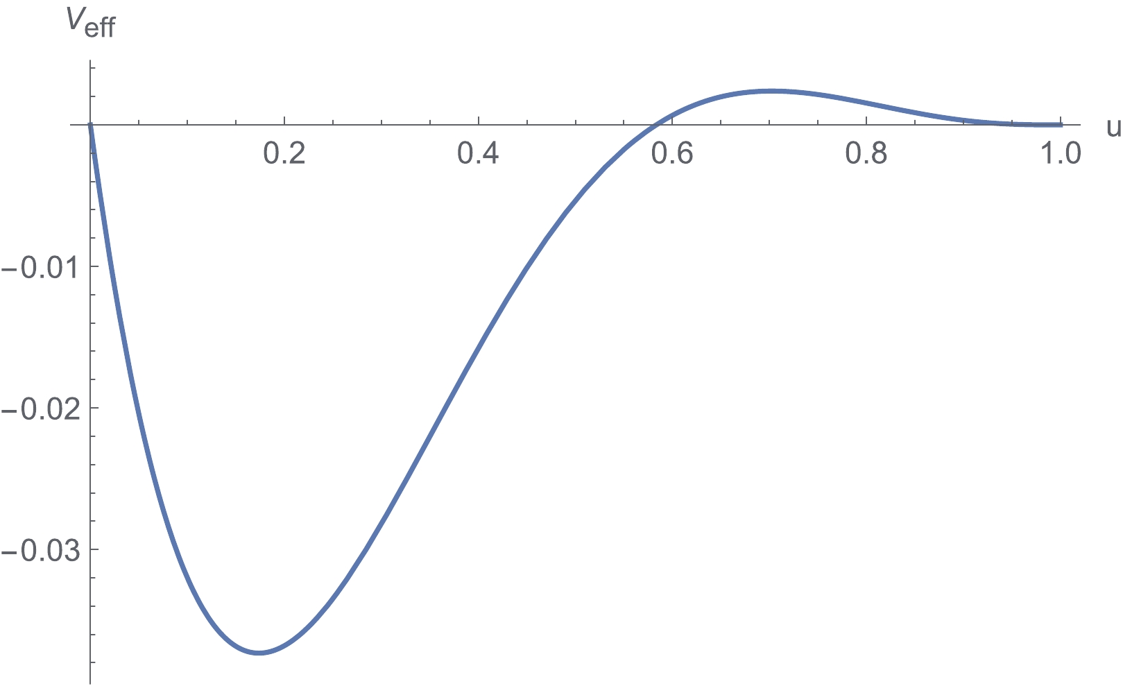
Figure 1. (color online) Effective potential with the compact coordinate
$ u=\dfrac{r-r_{h}}{r} $ . Here, we use the parameters$ M=1,Q=0.8 $ .The asymptotic behavior of Equation (7) is
$ \begin{array}{*{20}{l}} R(r) \sim \left\{ \begin{array}{ll} (r-r_{h})^{-{\rm i} \frac{r_{h}^{2}\omega}{r_{h}-r_-}} ,\ \ & r\rightarrow r_{h} \\ {\rm e}^{{\rm i}\omega r} r^{{\rm i}\omega} ,\ \ & r\rightarrow \infty \end{array} \right. \end{array} $

(9) which satisfies the purely ingoing boundary condition at the horizon and purely outgoing boundary condition at infinity. Here,
$ r_{-} $ is the radius of the inner horizon of the RN black hole. To implement the CFM, we obtain the Frobenius series as$ R(r)=(r-r_-)^{{\rm i}\omega} {\rm e}^{{\rm i}\omega r} \left( \frac{r-r_{h}}{r-r_-} \right)^{-{\rm i} \frac{r_{h}^{2}\omega}{r_{h}-r_-}} \sum_{k=0}^{\infty} a_{k} \left(\frac{r-r_{h}}{r-r_-}\right)^{k}. $

(10) Inserting (10) into (7), where the series is truncated to N, we obtain a complicated N-term recurrence relation on sequence (
$ a_{k} $ ), which can be numerically reduced to the$ 3 $ -term recurrence relation.$ \begin{aligned}[b] c^{(3)}_{0,i}a_{i}+c_{1,i}^{(3)}a_{i-1}+c_{2,i}^{(3)}a_{i-2}&=0, \quad \text{for} \; i>1, \\ c^{(3)}_{0,1}a_{1}+c_{1,1}^{(3)}a_{0} &= 0. \end{aligned} $

(11) The coefficients of (11) can be used to construct the continued fractions
$ g(\omega)=c^{(3)}_{1,1}-\frac{c^{(3)}_{0,1} c^{(3)}_{2,2}}{c^{(3)}_{1,2}- \dfrac{c^{(3)}_{0,2}c^{(3)}_{2,3}}{c^{(3)}_{1,3}- \cdots }}. $

(12) Fixing the parameters (
$ Q,b $ ),$ g(\omega) $ is zero if ω takes the values of the quasi-normal frequencies. The eigenvalue problem immediately becomes a problem of function$ g(\omega) $ searching for zeros on the complex ω plane. -
We depict the continued fraction values of
$ \log_{10}|g(\omega)| $ with respect to b on the complex plane when$ Q/M=0.8 $ in Fig. 2. For$ -b=2 $ , all the QNMs of the RN black hole in EMS theory have negative$ \omega_I $ values, i.e., there are no unstable modes. The first unstable mode appears when$ -b=5 $ . As$ -b $ increases further, more unstable modes appear. This is consistent with the analysis of the effective potential. The second unstable mode appears when$ -b=26 $ . All the unstable modes locate at the image axis, that is, they are purely imaginary modes.
Figure 2. (color online) Continued fraction values of the RN black hole in the EMS theory when
$ M=1,Q=0.8 $ . The left, middle, and right panels are for$ -b=2,5,10 $ , respectively. The quasinormal modes are located at the crosses.The parameter region in which RN black holes have unstable modes is shown in the left panel of Fig. 3. The unstable region obtained using linear perturbation is in good agreement with a similar figure presented in [30]. However, we cannot gain the unstable region beyond the critical charge
$ Q_{c}=1 $ because no definition exists of the asymptotic behavior for a bare singularity.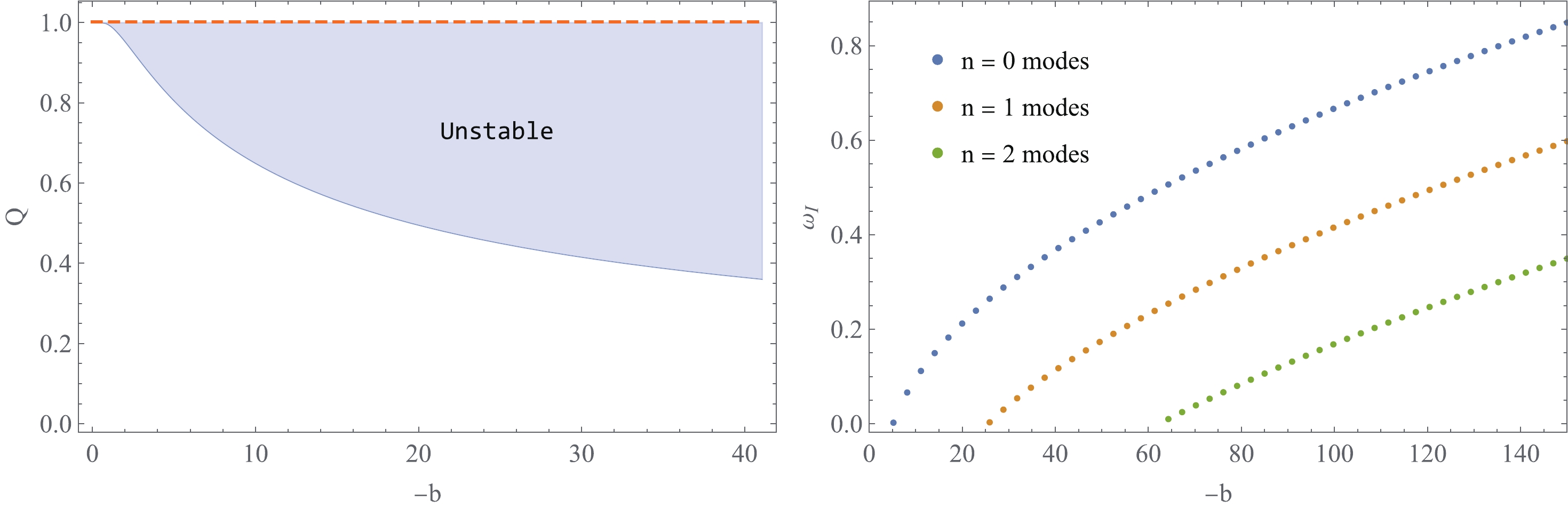
Figure 3. (color online) Left panel is the unstable region of parameter plane for
$ Q,-b $ . The right panel is the imaginary parts of unstable modes with different$ -b $ when fixing$ Q=0.8 $ .The imaginary parts of the unstable modes with different
$ -b $ values are shown in the right panel of Fig. 3, where$ Q=0.8 $ . The first branch of unstable modes first appears while beyond the critical$ -b=5 $ . With increasing of$ -b $ , the second branch emerges at about$ -b=26 $ , and the third branch emerges at about$ -b=63 $ . These higher overtone modes are associated with the different bound states of the perturbation equation [50]. -
We simulate the nonlinear evolution of an EMS black hole in spherically symmetric spacetime by obtaining the Painlevé-Gullstrand (PG)-like coordinates ansatz
$ \begin{array}{*{20}{l}} {\rm d}s^{2} =-\left(1-\zeta^{2}\right)\alpha^{2}{\rm d}t^{2}+2\zeta\alpha {\rm d}t {\rm d}r+ {\rm d}r^{2}+r^{2}({\rm d}\theta^{2}+\sin^{2}\theta {\rm d}\phi^{2}). \end{array} $

(13) For the RN black hole,
$ \alpha=1,\zeta=\sqrt{\frac{2M}{r}-\frac{Q^{2}}{r^{2}}} $ . The PG coordinates have been used to study the black hole dynamics numerically [32, 34, 42, 44]. It is regular on the horizon and thus appropriate for the long-term simulation of the black hole dynamics. We obtain the gauge potential$ \begin{array}{*{20}{l}} A_{\mu}{\rm d}x^{\mu}=A(t,r){\rm d}t, \end{array} $

(14) and introduce following auxiliary variables:
$ \Phi=\partial_{r}\phi,\ \ \ P=\frac{1}{\alpha}\partial_{t}\phi-\zeta\Phi,\ \ \ E=\frac{1}{\alpha}\partial_{r}A. $

(15) From the Maxwell equations (4), we obtain
$ \begin{array}{*{20}{l}} \partial_{r}\left(r^{2}f(\phi)E\right)=0,\ \ \ \partial_{t}\left(r^{2}f(\phi)E\right)=0. \end{array} $

(16) Subsequently, we obtain
$ E=\frac{Q}{r^{2}f(\phi)}, $

(17) in which Q is a constant interpreted as the electric charge. The Einstein equations become
$ \partial_r\alpha= -\frac{rP\Phi\alpha}{\zeta}, $

(18) $ \partial_r\zeta= \frac{r}{2\zeta}\left(\Phi^{2}+P^{2}+\Lambda\right)+\frac{Q^{2}}{2r^{3}\zeta f(\phi)}+rP\Phi-\frac{\zeta}{2r}, $

(19) $ \partial_{t}\zeta= \frac{r\alpha}{\zeta}\left(P+\Phi\zeta\right)\left(P\zeta+\Phi\right). $

(20) The scalar field equation is given by
$ \begin{array}{*{20}{l}} \partial_{t}\phi =\alpha\left(P+\Phi\zeta\right), \end{array} $

(21) $ \partial_{t}P =\frac{\left(\left(P\zeta+\Phi\right)\alpha r^{2}\right)'}{r^{2}}+\frac{\alpha}{2}\frac{f'(\phi)Q^{2}}{r^{4}f^{2}(\phi)}. $

(22) We solve the system of equations (18)–(22) in the frame of fully nonlinear evolution. The numerical steps are shown in subsection IV.A and the results are presented in subsection IV.B. In the remainder of this paper, we fix
$ M=1 $ and$ Q=0.8 $ except where specifically mentioned. The Misner-Sharp mass is$ M_{\rm MS}(t,r)=\frac{r}{2}\left(1-g^{\mu\nu}\partial_{\mu}r\partial_{\nu}r\right)=\frac{r}{2}\zeta(t,r)^{2}, $

(23) which tends to be the spacetime mass when
$ r\to\infty $ . We also study the black hole irreducible mass$ M_{h}=\sqrt{\frac{A}{4\pi}} $ in which A is the area of the apparent horizon. -
Here, we first discuss the boundary conditions for the nonlinear equations of evolution. The auxiliary freedom in the metric ansatz (13) enables us to fix
$ \begin{array}{*{20}{l}} \alpha |_{r\rightarrow \infty} = 1 \end{array} $

(24) by rescaling the time coordinate. The other metric function ζ tends to
$ \sqrt{\dfrac{2M}{r}} $ when$ r \rightarrow \infty $ . We take the initial profile for the scalar field as$ \begin{array}{*{20}{l}} \phi = \kappa {\rm e}^{-(\frac{r-6 r_{h}}{r_{h}})^{2}} ,\ \ P=0, \end{array} $

(25) where
$ r_{h} $ is the horizon of the initial black hole solution, and κ is of order$ 10^{-7} $ such that we can neglect the back reaction of the scalar field to the initial background spacetime. Φ is given by (15). Plugging the initial$ \phi, \Phi, P $ into the constraint equation (19), the initial ζ can be obtained using the Newton-Raphson method. Subsequently, the initial α can be obtained from (18).Given parameters (
$ M, Q, b $ ), the boundary conditions, and initial profiles ($ \phi, \Phi, P, \zeta, \alpha $ ), the numerical simulation process is as follows: we obtain$ \zeta,\phi,P $ on the next time slice using (20, 21, 22); we can then obtain$ \Phi,\alpha $ from (15, 18). We iterate these procedure to gain all the following time slices.We calculate in the radial computational region ranges from
$ r_{0} $ to$ \infty $ , where$ r_{0}=0.7 r_{h} $ .$ r_{0} $ always lies in the apparent horizon, which is guaranteed by the initial apparent horizon$ r_{h} $ . In principle, the information would not affect the region outside the horizon. The computational region is compactified by a coordinate transformation$ z=\dfrac{r}{r+M} $ , which ranges at$ (z_{0},1) $ . We use the finite difference method in the radial direction and discrete the radial direction by a uniform grid with$ 2^{11}\sim 2^{12} $ points. We evolve the system through the fourth-order Runge-Kutta method. We also use the Kreiss-Oliger dissipation to stabilize the numerical evolution. -
We first investigate the final value
$ \phi_{f} $ of the scalar field and the black hole irreducible mass$ M_{f} $ with respect to$ -b $ . The results are shown in Fig. 4. The scalar is inhibited while$ -b $ is below the critical value$ -b=5 $ , and we can deduce that this system evolves into the RN black hole. A similar scenario occurs in the final irreducible mass$ M_{f} $ . When$ -b $ exceeds the critical value,$ \phi_{f} $ increases rapidly and then decreases with$ -b $ . This shows that the scalar field absorbs electromagnetic energy through the coupling term${\rm e}^{-b\phi^{2}}F_{\mu\nu}F^{\mu\nu}$ .$ M_{f} $ increases monotonically with$ -b $ , which means that more energy of the scalar field is absorbed by the black hole for stronger coupling.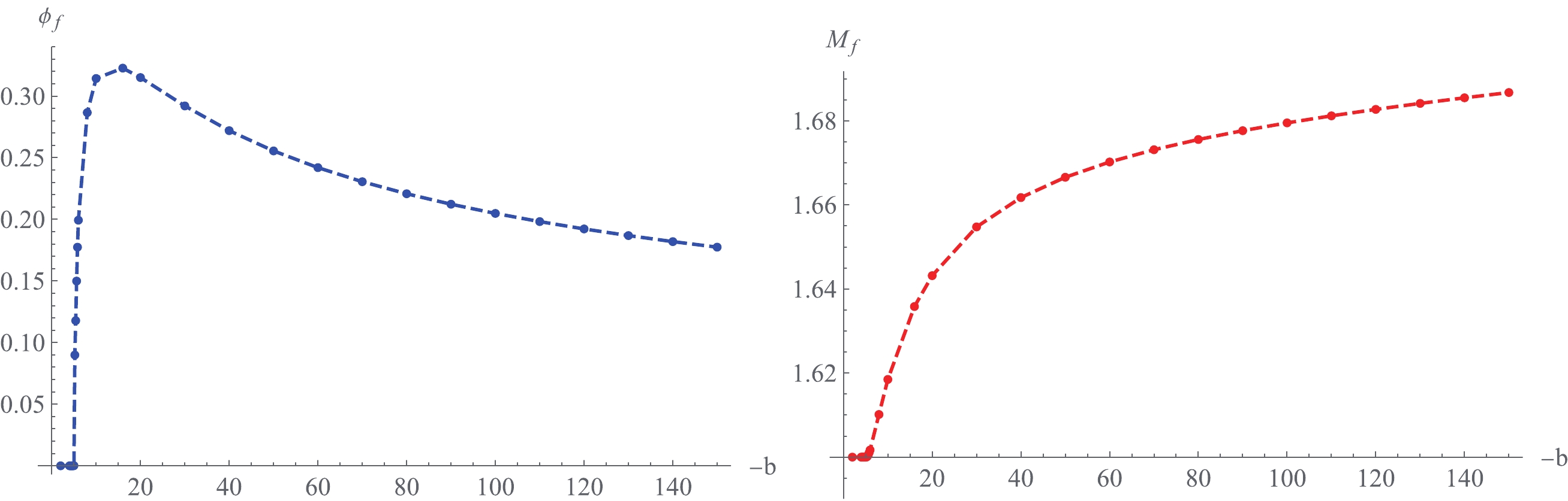
Figure 4. (color online) Final value of scalar field (left) and irreducible mass (right) at the horizon.
In Fig. 5, we show the radial profiles of the scalar field ϕ and the Misner-Sharp mass
$M_{\rm MS}$ in the final state. The scalar field condenses near the horizon, which is more apparent with small$ -b $ values, and the Misner-Sharp mass distribution confirms this. Hence, the coupling term$-\frac{b}{2}\phi \: {\rm e}^{-b\phi^{2}}F_{\mu\nu}F^{\mu\nu}$ of equation (3) generates an effective repulsive potential. This potential decreases rapidly with r in the form of${\rm e}^{-b\phi^{2}}$ and drives away the scalar field from the black hole. This effect is enhanced by larger$ -b $ values, which can be used to explain the decay with large$ -b $ of the final value of$ \phi_{h} $ in the left panel of Fig. 4.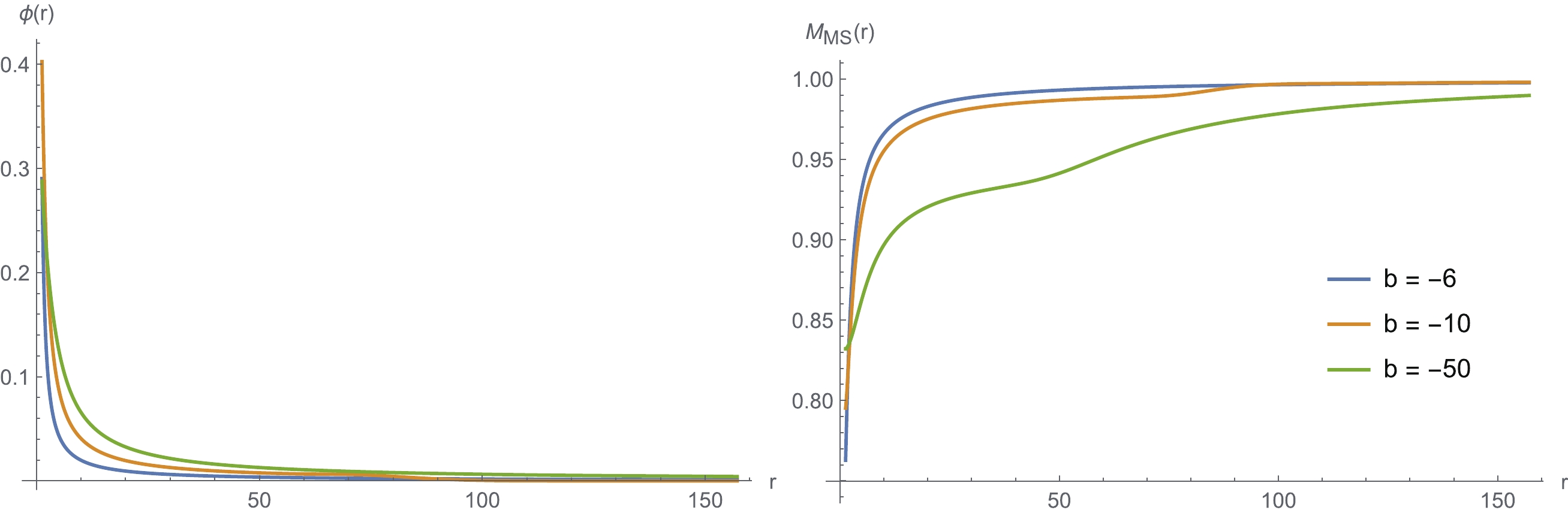
Figure 5. (color online) Left and right plots are the final profile of the scalar field and the Misner-Sharp mass with different b values, respectively.
The evolution of the scalar field
$ \phi_{h} $ on the apparent horizon and the irreducible mass$ M_{h} $ share the same characteristics as shown in Fig. 6. We take multiple perspectives to observe the evolution of the scalar field and effectively distinguish each evolution stage by comparing it with linear perturbation. The scalar field has three evolutionary stages: wave packet transmission, exponential growth, and oscillation convergence, which are denoted by thick, dashed, and thin lines, respectively.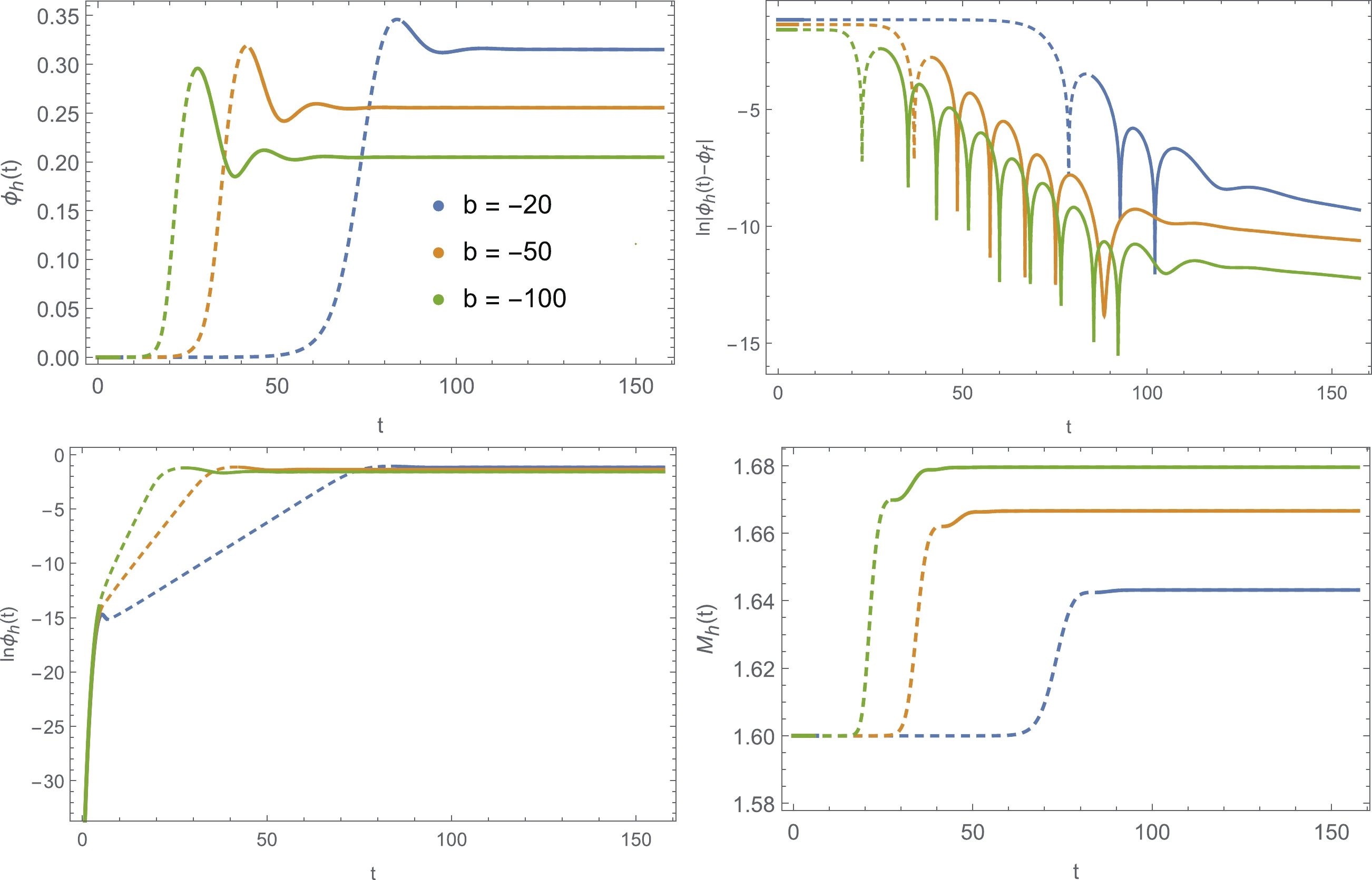
Figure 6. (color online) Upper left plot is the evolution of the scalar field at the horizon; the upper right plot is the logarithm of
$ |\phi_{h}-\phi_{f}| $ vs t; the lower left plot is the logarithm of the scalar vs t; the lower right plot is the irreducible mass at the horizon with time evolution. All plots share the same time interval, and the three line markers represent different evolutionary stages.At the early time, the evolution values (
$ \phi_{h},M_{h} $ ) are dominated by the propagation of the initial wave packet, which corresponds to the early evolution of Fig. 6. The clearer figure is depicted in the left panel of Fig. 7, which is the radial waveform at the early time. The initial wave packet is separated into two parts: the ingoing wave approaches the event horizon and increases with time; the outgoing wave dissipates to infinity. When the wave packet has reached the horizon, the scalar field increases exponentially, which corresponds to the dashed line segments in Fig. 6. The irreducible mass of a black hole also increases exponentially. The scalar evolution in this stage can be fitted well by the exponential function${\rm e}^{\omega_I t}$ . A comparison between$ \omega_I $ from the nonlinear evolution and the fundamental modes from the linear perturbation is shown in Fig. 8 with different$ -b $ values. This excellent coincidence indicates that the exponential growth at this stage is dominated by the unstable mode for linear perturbation.
Figure 7. (color online) Profile of
$ \phi(r) $ at the early time (left) and the remaining time (right), where we fix$ -b=50 $ .
Figure 8. (color online) Comparison between the fitting slope (blue) for the nonlinear evolution and the fundamental modes (red) for the linear perturbation with different
$ -b $ values.The third stage begins after the highest point of each line in the upper left panel of Fig. 6. It corresponds to a decaying oscillation period, which is clear in the upper left and upper right panels of Fig. 6. In the right panel of Fig. 7, when the scalar reaches its maximum (the brown line at time
$ t=40.3293 $ ), the scalar field gathers in a very narrow range near the event horizon. Thereafter, the value of the scalar falls back and spreads to infinity. Part of the energy of the scalar field is absorbed by the black hole, which increases the black hole area again as in the lower right panel of Fig. 6. -
We analyzed the linear scalar perturbation of the RN black hole in the EMS theory with the nonlinear coupling function
${\rm e}^{-b\phi^2}$ . The nonlinear coupling introduces a negative potential well for the scalar outside the horizon for negative b. When the radial integration of the effective potential of the scalar is negative, the tachyonic instability can be triggered. It drives the system away from the scalar-free RN solution, resulting in a scalarized charged black hole solution. Most of the scalar is accumulated in the potential well. The potential well increases with$ -b $ . Thus, the black hole is dressed heavier for larger$ -b $ values. We analyzed the QNM structure of the scalar perturbation using the continued fraction method. All the unstable modes have a purely imaginary part. For large$ -b $ values, the overtones can also be unstable. We obtain the unstable parameter region of the RN black hole in the EMS theory. It is in good agreement with that obtained in [30].We also studied the fully nonlinear evolution of the unstable RN black hole after a small perturbation in the EMS theory. The evolution endpoint of scalar field
$ \phi_{f} $ and irreducible mass$ M_{f} $ with different b are presented. We show the radial distribution of$ \phi(r) $ and$ M_{ \text{MS}}(r) $ of the final state. Through four different perspectives, we conclude that the scalar evolution can be divided into three stages: wave packet transmission, exponential growth, and oscillation convergence. The exponential coefficient of the second stage coincides well with the unstable mode from the linear analysis. We observe that the fundamental unstable mode dominates this stage and the overtones do not. The third stage can be considered the perturbation of the final scalarized black hole. -
Peng Liu would like to thank Yun-Ha Zha for her kind encouragement during this work.
Dynamical spontaneous scalarization in Einstein-Maxwell-scalar theory
- Received Date: 2022-04-05
- Available Online: 2022-09-15
Abstract: We study the linear instability and nonlinear dynamical evolution of the Reissner-Nordström (RN) black hole in the Einstein-Maxwell-scalar theory in asymptotic flat spacetime. We focus on the coupling function


 DownLoad: