


 Abstract
 HTML
HTML Reference
 Related
 PDF
PDF


-
The anomalous magnetic dipole moment (MDM) of a muon,
$ a_\mu=(g_\mu-2)/2 $ , has recently been measured by the Muon g-2 experiment at Fermilab [1−4], which reported that the result is 3.3 standard deviations (σ) greater than the standard model (SM) prediction based on its Run-1 data and is in agreement with the previous Brookhaven National Laboratory (BNL) E821 measurement [5]. Combined with previous E821 measurements, the new experimental average for the difference between the experimental measurements and the SM prediction [6] of$ a_\mu $ is given by$ \begin{array}{*{20}{l}} \Delta a_{\mu}=a_{\mu}^{\rm exp}-a_{\mu}^{\rm SM}=(25.1\pm5.9)\times10^{-10}, \end{array} $

(1) which increases the difference between the experimental measurements and the SM theoretical prediction to 4.2σ. This result will further motivate the development of SM extensions. There are many research papers on the muon anomalous MDM, such as Refs. [7−92] and the references therein. However, it is worth mentioning that the latest result obtained by a lattice QCD calculation [93] of the leading order hadronic vacuum polarization contribution to
$ a_\mu $ is larger than the previous result, which can accommodate the discrepancy between the experiment and the SM prediction, hence the discrepancy needs further scrutiny.In this work, we will analyze the muon anomalous MDM at the two-loop level in the μ from the ν Supersymmetric Standard Model (
$ \mu\nu $ SSM) [94−100], combined with the new experimental average. Through introducing three singlet right-handed neutrino superfields$ \hat{\nu}_i^c $ ($ i=1,2,3 $ ), the μνSSM can be used to solve the μ problem [101] of the minimal supersymmetric standard model (MSSM) [102−106], and can generate three tiny neutrino masses through a TeV scale seesaw mechanism [95, 107−113].The corresponding superpotential of the μνSSM is given as [94, 95]
$ \begin{aligned}[b] W=&{\epsilon _{ab}}\left( {Y_{{u_{ij}}}}\hat H_u^b\hat Q_i^a\hat u_j^c + {Y_{{d_{ij}}}}\hat H_d^a\hat Q_i^b\hat d_j^c + {Y_{{e_{ij}}}}\hat H_d^a\hat L_i^b\hat e_j^c \right) \\ & + {\epsilon _{ab}}{Y_{{\nu _{ij}}}}\hat H_u^b\hat L_i^a\hat \nu _j^c - {\epsilon _{ab}}{\lambda _i}\hat \nu _i^c\hat H_d^a\hat H_u^b + \frac{1}{3}{\kappa _{ijk}}\hat \nu _i^c\hat \nu _j^c\hat \nu _k^c. \end{aligned} $

(2) where
$ a,b=1,2 $ are SU(2) indices with the antisymmetric tensor$ \epsilon_{12}=1 $ , and$ i,j,k=1,2,3 $ are generation indices. The repeating indices imply the following summation convention.$ Y_{u,d,e,\nu} $ , λ, and κ are dimensionless matrices, a vector, and a symmetric tensor, respectively. In the superpotential, the effective bilinear terms$ \epsilon _{ab} \varepsilon_i \hat H_u^b\hat L_i^a $ and$ \epsilon _{ab} \mu \hat H_d^a\hat H_u^b $ can be generated with$ \varepsilon_i= Y_{\nu _{ij}} \langle {\tilde \nu _j^c} \rangle $ and$ \mu = {\lambda _i}\langle {\tilde \nu _i^c} \rangle $ once the electroweak symmetry is broken. The general soft SUSY-breaking terms, the usual D- and F-term contributions of the tree-level scalar potential, and the mass matrices of the particles in the μν SSM can be seen in Refs. [95, 96, 99]. In the μνSSM, the gravitino or the axino can be dark matter candidates [95, 96, 110, 114−119].In our previous work, the Higgs boson mass and decay modes
$ h\rightarrow \gamma\gamma $ ,$ h\rightarrow VV^* $ ($ V=Z,W $ ),$ h\rightarrow f\bar{f} $ ($ f=b,\tau $ ), and$ h\rightarrow Z\gamma $ in the$ \mu\nu $ SSM were researched [120−124]. Constrained by the 125 GeV Higgs boson mass and decays, herein we will investigate the anomalous MDM of the charged leptons at the two-loop level in the$ \mu\nu $ SSM, combined with the updated experimental average of the muon MDM. For the electron anomalous MDM,$ a_e=(g_e-2)/2 $ , the experimental result showed a negative$ \sim2.4\sigma $ discrepancy between the measured value [125] and the SM prediction [126]. However, a new determination of the fine structure constant with a higher accuracy [127], obtained from a measurement of the recoil velocity on rubidium atoms, resulted in a re-evaluation of$ a_e $ in the SM, revising it to a positive$ \sim1.6\sigma $ discrepancy$ \begin{array}{*{20}{l}} &&\bigtriangleup a_e\equiv a_e^{\rm exp}-a_e^{\rm SM}=(4.8\pm3.0)\times10^{-13}. \end{array} $

(3) Interestingly, now
$ \bigtriangleup a_e $ and$ \bigtriangleup a_\mu $ are all positive.Now, the measured averages of the signal strengths for the 125 GeV Higgs boson decays into two taus and bottom quarks relative to the standard model (SM) prediction are respectively
$ 1.15^{+0.16}_{-0.15} $ and$ 1.04\pm0.13 $ with high experimental precision [128]. Although Higgs boson decays into a pair of fermions of the third generation can now be measured accurately by the Large Hadron Collider (LHC), the Higgs boson decays into a pair of fermions of the first or second generation are challenging to measure, as the Yukawa couplings of the 125 GeV Higgs boson to fermions of the first and second generation are smaller than that of the third generation. However, the ATLAS and CMS Collaborations recently measured the 125 GeV Higgs boson decay into a pair of muons$ h\rightarrow \mu \bar{\mu} $ , and reported that the signal strength relative to the SM prediction is$ 1.2\pm0.6 $ with 2.0σ [129] and$ 1.19^{+0.40+0.15}_{-0.39-0.14} $ with 3.0σ [130], respectively. The dimuon decay of the 125 GeV Higgs boson$ h\rightarrow \mu \bar{\mu} $ offers the best opportunity for measuring Higgs interactions with second-generation fermions at the LHC. The 125 GeV Higgs boson decay$ h\rightarrow \mu \bar{\mu} $ has been discussed within various theoretical frameworks [131−143]. Herein, we investigate the 125 GeV Higgs boson decay$ h\rightarrow \mu \bar{\mu} $ at the one-loop level in the$ \mu\nu $ SSM.In the following, we briefly introduce the MDM of the charged leptons in Sec. II. In Sec. III, we give the decay width of the 125 GeV Higgs boson decays into a pair of charged leptons
$ h\rightarrow l_i \bar{l}_i $ at the one-loop level. Sec. IV and Sec. V respectively show the numerical analysis and summary. -
The MDM of the charged leptons in the
$ \mu\nu $ SSM can be written by the effective Lagrangian$ \mathcal{L}_{\rm MDM}={e\over 4m_{l_i}}a_{l_i}\overline{l}_{i}\sigma^{\alpha \beta}l_{i}F_{\alpha \beta}, $

(4) where
$ l_i $ represents the charged leptons, which are on-shell,$ m_{l_i} $ is the mass of the charged leptons,$ \sigma^{\alpha\beta}=({\rm i}/{2})[\gamma^\alpha,\gamma^\beta] $ ,$ F_{\alpha\beta} $ denotes the electromagnetic field strength and the MDM of the charged leptons is$ a_{l_i}=({1}/{2})(g_{l_i}-2) $ . Including the main two-loop electroweak corrections, the MDM of the charged leptons in the$ \mu\nu $ SSM can be given by$ \begin{array}{*{20}{l}} &&a_{l_i}^{\rm{SUSY}}=a_{l_i}^{\rm{one-loop}}+a_{l_i}^{\rm{two-loop}}, \end{array} $

(5) where the one-loop corrections
$ a_{l_i}^{\rm{one-loop}} $ are pictured in Fig. 1 and the main two-loop corrections$ a_{l_i}^{\rm{two-loop}} $ are shown in Fig. 2.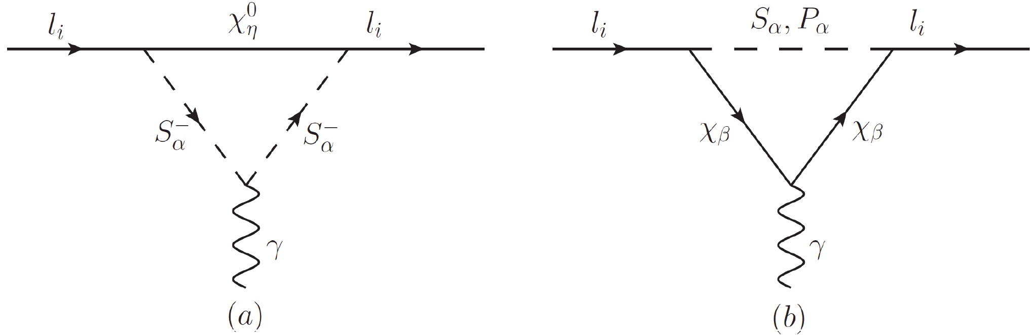
Figure 1. Dominant one-loop diagrams representing the contributions from neutral fermions
$ \chi_\eta^0 $ and charged scalar$ S_{ \alpha}^- $ loops (a), and the contributions from charged fermions$ \chi_\beta $ and neutral scalar$ S_{ \alpha} $ (or$ P_{ \alpha} $ ) loops (b).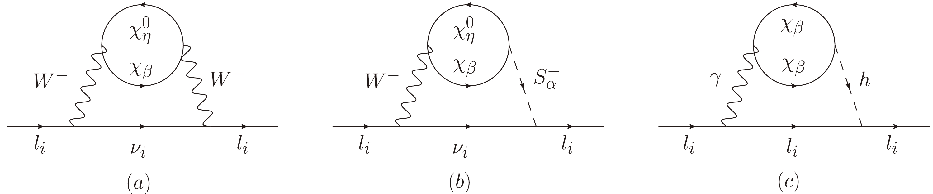
Figure 2. Main two-loop rainbow diagram (a) and Barr-Zee type diagrams (b, c).
In Fig. 1, the contributions of the charged leptons to the MDM at the one-loop level in the
$ \mu\nu $ SSM come from neutral fermions and charged scalar loops (neutral fermions$ \chi_{\eta}^{0} $ and charged scalars$ S_{ \alpha}^- $ are loop particles) and the charged fermions and neutral scalar loop (charged fermions$ \chi_{\beta} $ and neutral scalars$ N_\alpha=S_{ \alpha},P_{ \alpha} $ are loop particles). The concrete expressions of the one-loop corrections$ a_{l_i}^{\rm{one-loop}} $ can be found in our previous related work [122] by replacing the charged leptons$ {l_i} $ with the muon$ {l_\mu} $ .Here, the dominant contribution of the muon MDM
$ a_\mu $ comes from the charged fermions and neutral scalar loops in Fig. 1(b). We check that the one-loop correction in the$ \mu\nu $ SSM is approximately in agreement with the MSSM and the Next-to-Minimal Supersymmetric Standard Model (NMSSM) [10, 64, 82]. Although the MDM of the muon in the$ \mu\nu $ SSM has roughly the same properties in the MSSM and NMSSM, it is subject to significantly relaxed limitations in parameter space in the$ \mu\nu $ SSM if other physical quantities are researched. Of course, through introducing three singlet right-handed neutrino superfields$ \hat{\nu}_i^c $ ($ i=1,2,3 $ ) for solving the μ problem of the MSSM and generating three tiny neutrino masses, the μνSSM still can give some additional contributions to the muon MDM$ a_\mu $ beyond the MSSM.In Fig. 2, the main two-loop rainbow diagram (a) and the Barr-Zee type diagrams (b, c) of
$ a_{l_i} $ in the$ \mu\nu $ SSM are shown, in which a closed fermion loop is attached to virtual gauge bosons or scalars, and the corresponding corrections for$ a_{l_i} $ are obtained by attaching a photon in all possible ways to the internal particles. In our previous work [123], we show the main two-loop contributions of the muon MDM in the approximation$ m_{\chi_{\eta}^{0}}\simeq m_{\chi_{\beta}} $ . In this paper, we give the main two-loop contributions$ a_{l_i}^{\rm{two-loop}} $ for the general case.In the
$ \mu\nu $ SSM, the main SUSY two-loop corrections of the MDM of the charged leptons can be given as$ \begin{array}{*{20}{l}} a_{l_i}^{\rm{two-loop}}=a_{l_i}^{WW}+a_{l_{i}}^{WS}+a_{l_i}^{\gamma h}, \end{array} $

(6) where the terms
$ a_{l_i}^{WW},a_{l_i}^{WS},a_{l_i}^{\gamma h} $ are the contributions corresponding to Figs. 2 (a−c). The contribution from the main two-loop rainbow diagram in Fig. 2(a) can be written as$ \begin{aligned}[b] a_{l_i}^{WW}=&{G_{_F}m_{l_i}^2\over 8\sqrt{2}\pi^4} \Bigg\{\Bigg(\Big|C_{\rm L}^{W \overline{\chi}_{\eta}^{0}\chi_{\beta}}\Big|^2+\Big|C_{\rm R}^{W\overline{\chi}_{\eta}^{0}\chi_{\beta}}\Big|^2\Bigg) T_1(1,x_{{\chi_{\eta}^{0}}},x{_{\chi_\beta}})\\ & +\Bigg(\Big|C_{\rm L}^{W\overline{\chi}_{\eta}^{0}\chi_{\beta}}\Big|^2-\Big|C_{\rm R}^{W\overline{\chi}_{\eta}^{0}\chi_{\beta}}\Big|^2\Bigg) T_2(1,x_{{\chi_{\eta}^{0}}},x_{{\chi_\beta}}) \end{aligned} $

$ \begin{aligned}[b]\quad\quad\quad +2(x_{{\chi_{\eta}^{0}}}x_{{\chi_\beta}})^{1/2}\Re\Big(C_{\rm R}^{W\overline{\chi}_{\eta}^{0}\chi_{\beta}*} C_{\rm L}^{W\overline{\chi}_{\eta}^{0}\chi_{\beta}}\Big)T_3(1,x_{{\chi_{\eta}^{0}}},x{_{\chi_\beta}})\Bigg\}\;, \end{aligned} $

(7) with
$ x_i=m_i^2/m_W^2 $ . The expressions of the form factors$ T_i $ can be found in Refs. [144−146]. The concrete expressions for couplings C in the$ \mu\nu $ SSM can be seen in Ref. [99].The contribution from the main two-loop Barr-Zee type diagram in Fig. 2 (b) can be given by
$ \begin{aligned}[b] a_{l_{i}}^{WS}=&{G_{\rm F}m_{l_{i}}m_{W}\over128\pi^4g_2}\Re{( C_{\rm L}^{S_{ \alpha}^-\overline{l}_i{\chi_{7+i}^0}} )}\\ & \times\Bigg\{(x_{{\chi_\beta}})^{1/2} F_1(1,x_{S_{\alpha}^-},x_{{\chi_{\eta}^{0}}},x_{{\chi_\beta}}) \\&\times\Re\Big(C_{\rm L}^{S_{ \alpha}^-\overline\chi_{\beta}{\chi}_{\eta}^{0}}C_{\rm L}^{W \overline{\chi}_{\eta}^{0}\chi_{\beta}}+C_{\rm R}^{S_{ \alpha}^-\overline\chi_{\beta}{\chi}_{\eta}^{0}}C_{\rm R}^{W \overline{\chi}_{\eta}^{0}\chi_{\beta}}\Big) \\ & +(x_{{\chi_{\eta}^{0}}})^{1/2} F_2(1,x_{{S_{ \alpha}^-}},x_{{\chi_{\eta}^{0}}},x_{{\chi_\beta}})\\& \times\Re\Big(C_{\rm L}^{S_{ \alpha}^-\overline\chi_{\beta}{\chi}_{\eta}^{0}}C_{\rm R}^{W \overline{\chi}_{\eta}^{0}\chi_{\beta}}+C_{\rm R}^{S_{ \alpha}^-\overline\chi_{\beta}{\chi}_{\eta}^{0}}C_{\rm L}^{W \overline{\chi}_{\eta}^{0}\chi_{\beta}}\Big) \\ & +(x_{{\chi_\beta}})^{1/2} F_3(1,x_{S_{ \alpha}^-},x_{{\chi_{\eta}^{0}}},x_{{\chi_\beta}}) \\&\times\Re\Big(C_{\rm L}^{S_{ \alpha}^-\overline\chi_{\beta}{\chi}_{\eta}^{0}}C_{\rm L}^{W \overline{\chi}_{\eta}^{0}\chi_{\beta}}-C_{\rm R}^{S_{ \alpha}^-\overline\chi_{\beta}{\chi}_{\eta}^{0}}C_{\rm R}^{W \overline{\chi}_{\eta}^{0}\chi_{\beta}}\Big) \\ & +(x_{{\chi_{\eta}^{0}}})^{1/2} F_4(1,x_{S_{ \alpha}^-},x_{{\chi_{\eta}^{0}}},x_{{\chi_\beta}})\\& \times\Re\Big(C_{\rm L}^{S_{ \alpha}^-\overline\chi_{\beta}{\chi}_{\eta}^{0}}C_{\rm R}^{W \overline{\chi}_{\eta}^{0}\chi_{\beta}}-C_{\rm R}^{S_{ \alpha}^-\overline\chi_{\beta}{\chi}_{\eta}^{0}}C_{\rm L}^{W \overline{\chi}_{\eta}^{0}\chi_{\beta}}\Big)\Bigg\}\;, \end{aligned} $

(8) where the expressions of the form factors
$ F_{i} $ can be seen in Ref. [144]. Here, in the$ \mu\nu $ SSM, h denotes$ S_{ 1} $ ,$ l_i $ is denoted by$ {\chi}_{2+i} $ . Considering that the masses of the charged scalars$ S_{ \alpha}^{-} $ are larger than the mass of a W gauge boson constrained by the present experiments, the contribution from the main two-loop Barr-Zee type diagram$ a_{l_{i}}^{WS} $ is smaller than the contribution from the main two-loop rainbow diagram$ a_{l_i}^{ WW} $ .The contribution from the main two-loop Barr-Zee type diagram in Fig. 2(c) can be written as
$ a_{l_{i}}^{\gamma h}={{-G_{\rm F} m_{l_i}m_{W} s_W^2} \over {16\pi^4}}(x_{{\chi_\beta}})^{1/2} T_{11}(x_{{h}},x_{{\chi_{\beta}}},x_{{\chi_{\beta}}})\Re\Big(C_{\rm L}^{h \overline{l}_i {l}_{i}} C_{\rm L}^{h\overline{\chi}_{\beta}{\chi}_{\beta}}\Big)\;. $

(9) Through the numerical calculation, normalized to the one-loop corrections
$ a_{l_i}^{\rm{one-loop}} $ , the two-loop corrections of the MDM$ a_{l_i}^{\rm{two-loop}} $ in the$ \mu\nu $ SSM may reach about 10$ \% $ , when$ \tan\beta $ is large, and the masses of the superpartners are small and constrained by the experiments. Therefore, one-loop correction alone is sufficient for explaining the g-2 of a muon and satisfying all other experimental constraints. In the following numerical analysis, the two-loop corrections of the muon MDM are still considered to be more precise. -
The corresponding effective amplitude for the 125 GeV Higgs decay
$ h\rightarrow l_i \bar{l}_i $ can be written as$ \mathcal{M}= h{\bar l_i}({F_{\rm L}^{i}}{P_{\rm L}} + {F_{\rm R}^{i}}{P_{\rm R}}){l_i}. $

(10) The decay width of
$ h\rightarrow l_i\bar{l}_i $ can be obtained as$ {\Gamma}(h\rightarrow l_i\bar{l}_i) \simeq \frac{m_h}{16\pi}\Big({\left| {F_{\rm L}^{i}} \right|^2} + {\left| {F_{\rm R}^{i}} \right|^2}\Big). $

(11) The contribution from the tree level in the
$ \mu\nu $ SSM can be written as$ F_{\rm L}^{({\rm tree})i}=F_{\rm R}^{({\rm tree})i} = \frac{m_{l_i}}{\sqrt{2}\upsilon\cos \beta}R_{S_{ 11}}, $

(12) where
$ m_{l_i} $ denotes the mass of the lepton$ l_i $ ,$ \upsilon\simeq174 $ GeV, and$ R_S $ is the unitary matrix which diagonalizes the mass matrix of CP-even neutral scalars [120]. In the SM, the contribution from the tree level can be written by$ F_{{\rm L}(\rm{SM})}^{({\rm tree})i}=F_{{\rm R}(\rm{SM})}^{({\rm tree})i} = \frac{m_{l_i}}{\sqrt{2}\upsilon}. $

(13) The running lepton masses
$ m_{l_i}(\Lambda) $ are related to the pole masses$ m_{l_i} $ through [147]$ m_{l_i}(\Lambda)=m_{l_i}\Bigg\{ 1-\frac{\alpha(\Lambda)}{\pi} \Bigg[1+\frac{3}{4} \ln \frac{\Lambda^2}{m_{l_i}^2}\Bigg]\Bigg\}. $

(14) Similarly to the decays
$ h\rightarrow l_i\bar{l}_i $ , the decay width of the 125 GeV Higgs decay into down-type quarks$ h\rightarrow d_i \bar{d}_i $ can be given as$ {\Gamma}(h\rightarrow d_i \bar{d}_i) \simeq \frac{N_c m_h}{16\pi}\Big({\left| {F_{dL}^{i}} \right|^2} + {\left| {F_{dR}^{i}} \right|^2}\Big), $

(15) with
$ N_c=3 $ , and the tree level contribution in the$ \mu\nu $ SSM is$ F_{dL}^{({\rm tree})i}=F_{dR}^{({\rm tree})i} = \frac{m_{d_i}}{\sqrt{2}\upsilon\cos \beta}R_{S_{ 11}}, $

(16) where
$ m_{d_i} $ denotes the mass of the down-type quarks$ d_i $ . In the SM, the contribution from the tree level can be written by$ F_{dL(\rm{SM})}^{({\rm tree})i}=F_{dR(\rm{SM})}^{({\rm tree})i} = \frac{m_{d_i}}{\sqrt{2}\upsilon}. $

(17) The difference between the decay width of
$ h\rightarrow f_i \bar{f}_i $ of the$ \mu\nu $ SSM ($ {\Gamma}_{\rm{NP}}(h\rightarrow f_i \bar{f}_i) $ ) and that of the SM ($ {\Gamma}_{\rm{SM}}(h\rightarrow f_i \bar{f}_i) $ ) in the tree level can be given as$ \delta_{\rm tree}\equiv {{\Gamma}_{\rm{NP}}(h\rightarrow f_i \bar{f}_i)-{\Gamma}_{\rm{SM}}(h\rightarrow f_i \bar{f}_i)\over {\Gamma}_{\rm{SM}}(h\rightarrow f_i \bar{f}_i)}=\frac{R_{S_{ 11}}^2}{\cos^2 \beta}-1. $

(18) Here,
$ f_i=l_i,\,d_i $ , due to the fact that the tree-level contribution of the Higgs boson decay into leptons is identical to that for the Higgs boson decay into down-tpye quarks. The numerical results can show that the ratio$ \delta_{\rm tree} $ is about$ 1\% $ when the parameter$ \tan\beta $ in the$ \mu\nu $ SSM is small.The one-loop electroweak correction for
$ h\rightarrow l_i\bar{l}_i $ in the SM is approximated by [133−137]$ {\Gamma}_{\rm SM}^{({\rm one})}(h\rightarrow l_i\bar{l}_i) \simeq {\Gamma}_{\rm SM}^{({\rm tree})}(h\rightarrow l_i\bar{l}_i)\delta_{\rm week}^{l}, $

(19) with
$ \begin{aligned}[b] \delta_{\rm week}^{l}=&\frac{G_{\rm F}}{8\pi^2 \sqrt{2}}\Bigg[ 7m_t^2 + m_W^2\Bigg(-5 + \frac{3\log{c_W^2}}{s_W^2} \Bigg) \\&- m_Z^2 \frac{6(1-8s_W^2+16s_W^4)-1}{2} \Bigg], \end{aligned} $

(20) where the contributions come from the t quark, W boson and Z boson. The numerical result shows that the one-loop electroweak contribution relative to the tree contribution
$ \delta_{\rm week}^{l} $ is about 1.7%.The one-loop diagrams for
$ h\rightarrow l_i\bar{l}_i $ in the$ \mu\nu $ SSM beyond the SM are depicted in Fig. 3. Then, the contributions from the one-loop diagrams in the$ \mu\nu $ SSM can be written by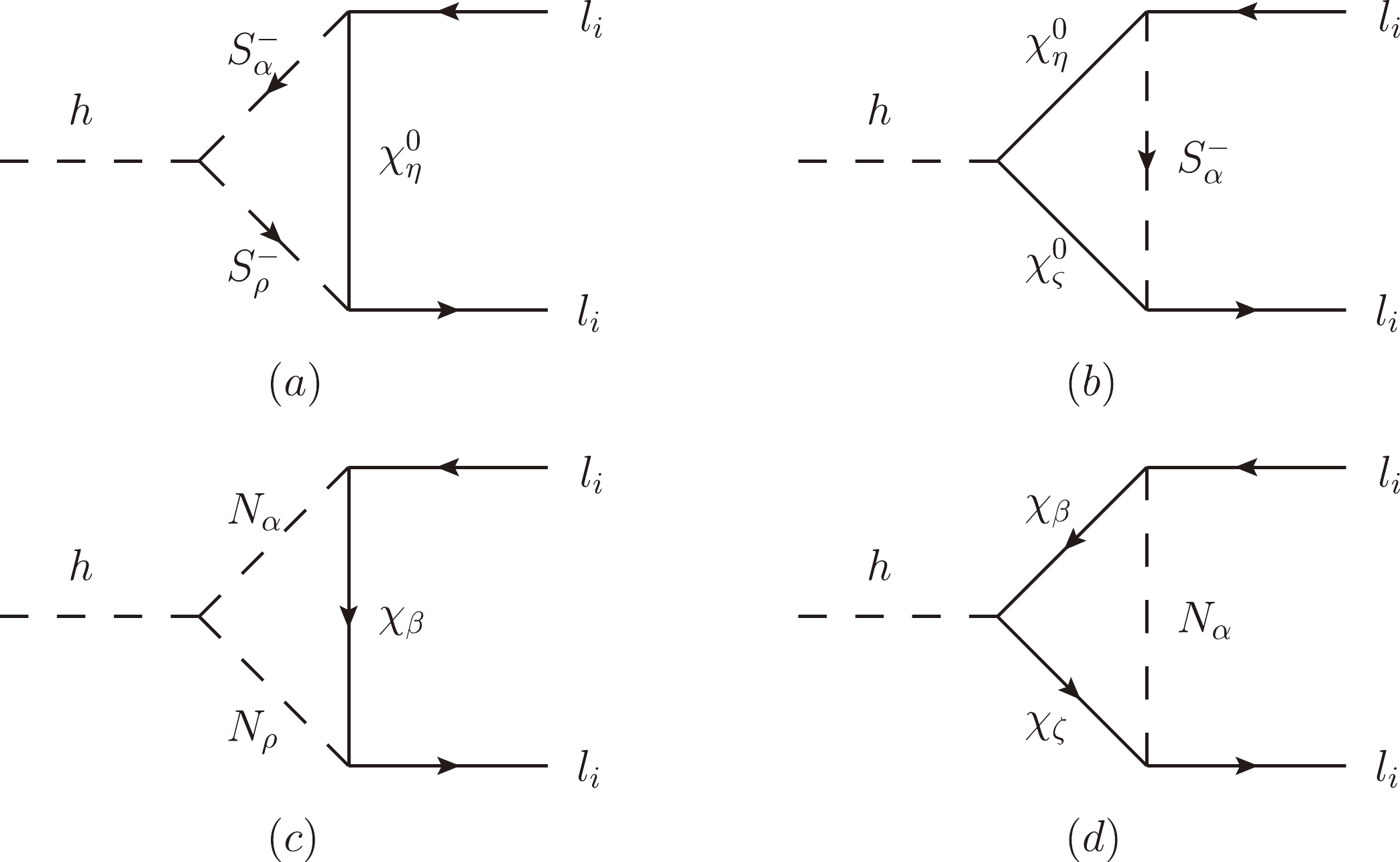
Figure 3. One-loop diagrams for
$ h\rightarrow l_i\bar{l}_i $ in the$ \mu\nu $ SSM. (a, b) represent the contributions from the charged scalar$ S_{\alpha,\,\rho}^- $ and neutral fermion$ \chi_{\eta,\varsigma}^0 $ loops, while (c, d) represent the contributions from the neutral scalar$ N_{\alpha,\,\rho} $ ($ N=S,P $ ) and charged fermion$ \chi_{\beta,\zeta} $ loops.$ \begin{array}{*{20}{l}} F_{\rm L,R}^{({\rm one})i} = F_{\rm L,R}^{(a)i} + F_{\rm L,R}^{(b)i} + F_{\rm L,R}^{(c)i} + F_{\rm L,R}^{(d)i}, \end{array} $

(21) where
$ F_{\rm L,R}^{(a,b)i} $ denotes the contributions from the charged scalar$ S_{ \alpha,\rho}^- $ and neutral fermion$ \chi_{\eta,\varsigma}^0 $ (upper index 0 shows neutral) loops, and$ F_{\rm L,R}^{(c,d)i} $ stands for the contributions from the neutral scalar$ N_{\alpha,\,\rho} $ ($ N=S,P $ ) and charged fermion$ \chi_{\beta,\zeta} $ loops.After integrating the heavy freedoms out, we formulate the neutral fermion loop contributions
$ F_{\rm L,R}^{(a,b)i} $ as follows:$ \begin{aligned}[b]F_{\rm L}^{(a)i} =& \frac{{m_{{\chi _\eta ^0}}}{C^{S^\pm}_{1 \alpha \rho }}}{{m_W^2}} C_{\rm L}^{S_\rho ^ - {{\bar l }_{i}} \chi _\eta ^0} C_{\rm L}^{S_\alpha ^{-\ast} \bar \chi _\eta ^0 {l_{i}}} {G_1}({x_{\chi _\eta ^0}},{x_{S_{ \alpha} ^ - }},{x_{S_\rho ^ - }}) ,\\ F_{\rm L}^{(b)i} = & \frac{{m_{{\chi _\varsigma^0 }}}{m_{{\chi _\eta^0 }}}}{{m_W^2}} C_{\rm L}^{{S_{ \alpha}^- }{{\bar l}_{i}}{\chi _\varsigma^0 }}C_{\rm L}^{h{{\bar \chi }_\varsigma^0 }{\chi _\eta^0 }} C_{\rm L}^{{S_{ \alpha}^{-\ast} }{{\bar \chi }_\eta^0}{l_{i}}}{G_1}({x_{{S_{ \alpha}^- }}},{x_{{\chi _\varsigma^0 }}},{x_{{\chi _\eta^0 }}})\\ & + \: C_{\rm L}^{{S_{ \alpha}^- }{{\bar l}_{i}}{\chi _\varsigma^0 }}C_{\rm R}^{h{{\bar \chi }_\varsigma^0 }{\chi _\eta^0 }} C_{\rm L}^{{S_\alpha^{-\ast} }{{\bar \chi }_\eta^0}{l_{i}}}{G_2}({x_{{S_{ \alpha}^- }}},{x_{{\chi _\varsigma^0 }}},{x_{{\chi _\eta^0 }}}) ,\\ F_{\rm R}^{(a,b)i} =& \left. {F_{\rm L}^{(a,b)i}} \right|{ _{{\rm L} \leftrightarrow {\rm R}}} . \end{aligned} $

(22) Here, the concrete expressions for the couplings C can be found in Refs. [121, 122], and the loop functions
$ G_{i} $ are given as$ \begin{aligned}[b] {G_1}({x_1 , x_2 , x_3}) = & \frac{1}{{16{\pi ^2}}}\Bigg[ \frac{{{x_1}\ln {x_1}}}{{({x_1} - {x_2})({x_1} - {x_3})}} + \frac{{{x_2}\ln {x_2}}}{{({x_2} - {x_1})({x_2} - {x_3})}} \\ & + \frac{{{x_3}\ln {x_3}}}{{({x_3} - {x_1})({x_3} - {x_2})}}\Bigg],\\[-10pt] \end{aligned} $

(23) $ \begin{aligned}[b] {G_2}({x_1 , x_2 , x_3}) = & \frac{1}{{16{\pi ^2}}}\Bigg[ \frac{{x_1^2\ln {x_1}}}{{({x_1} - {x_2})({x_1} - {x_3})}} + \frac{{x_2^2\ln {x_2}}}{{({x_2} - {x_1})({x_2} - {x_3})}} \\ & + \frac{{x_3^2\ln {x_3}}}{{({x_3} - {x_1})({x_3} - {x_2})}} \Bigg].\quad\;\; \\[-10pt]\end{aligned} $

(24) In a similar way, the charged fermion loop contributions
$ F_{\rm L,R}^{(c,d)i} $ are$ \begin{aligned}[b] F_{\rm L}^{(c)i} =& \sum\limits_{N=S,P} \frac{{m_{{\chi _\beta }}}{C^{N}_{1 \alpha \rho }}}{{m_W^2}} C_{\rm L}^{N_\rho {{\bar l }_{i}}\chi _\beta } C_{\rm L}^{N_\alpha \bar \chi _\beta {l_{i}} } {G_1}({x_{\chi _\beta }},{x_{N_\alpha }},{x_{N_\rho }}) ,\\ F_{\rm L}^{(d)i} =& \sum\limits_{N=S,P} \Big[ C_{\rm L}^{{N_\alpha }{{\bar l}_{i}}{\chi _\zeta }}C_{\rm R}^{h{{\bar \chi }_\zeta }{\chi _\beta }}C_{\rm L}^{{N_\alpha }{{\bar \chi }_\beta }{l_{i}}} {G_2}({x_{{N_\alpha }}},{x_{{\chi _\zeta }}},{x_{{\chi _\beta }}})\\ &+ \frac{{m_{{\chi _\zeta }}}{m_{{\chi _\beta }}}}{{m_W^2}} C_{\rm L}^{{N_\alpha }{{\bar l}_{i}}{\chi _\zeta }}C_{\rm L}^{h{{\bar \chi }_\zeta }{\chi _\beta }} C_{\rm L}^{{N_\alpha }{{\bar \chi }_\beta }{l_{i}}}{G_1}({x_{{N_\alpha }}},{x_{{\chi _\zeta }}},{x_{{\chi _\beta }}}) \Big],\\ F_{\rm R}^{(c,d)i} =& \left. {F_{\rm L}^{(c,d)i}} \right|{ _{{\rm L} \leftrightarrow {\rm R}}} . \end{aligned} $

(25) -
Firstly, we take some appropriate parameter space in the
$ \mu\nu $ SSM. For soft SUSY-breaking mass squared parameters, we make the minimal flavor violation (MFV) assumptions$ \begin{aligned}[b] &m_{\tilde Q_{ij}}^2 = m_{{{\tilde Q_i}}}^2{\delta _{ij}}, \quad m_{\tilde u_{ij}^c}^2 = m_{{{\tilde u_i}^c}}^2{\delta _{ij}}, \quad m_{\tilde d_{ij}^c}^2 = m_{{{\tilde d_i}^c}}^2{\delta _{ij}}, \\ &m_{{{\tilde L}_{ij}}}^2 = m_{{\tilde L}}^2{\delta _{ij}}, \quad m_{\tilde e_{ij}^c}^2 = m_{{{\tilde e}^c}}^2{\delta _{ij}}, \quad m_{\tilde \nu_{ij}^c}^2 = m_{\tilde \nu_{i}^c}^2{\delta _{ij}}, \end{aligned} $

(26) where
$ i,\;j,\;k =1,\;2,\;3 $ .$ m_{\tilde \nu_i^c}^2 $ can be constrained by the minimization conditions of the neutral scalar potential seen in Ref. [120]. For some coupling parameters, we also choose the MFV assumptions$ \begin{aligned}[b] &{\kappa _{ijk}} = \kappa {\delta _{ij}}{\delta _{jk}}, \quad {({A_\kappa }\kappa )_{ijk}} = {A_\kappa }\kappa {\delta _{ij}}{\delta _{jk}}, \quad \upsilon_{\nu_i^c}=\upsilon_{\nu^c}, \\& \lambda _i = \lambda,\quad {({A_\lambda }\lambda )}_i = {A_\lambda }\lambda,\quad {Y_{{e_{ij}}}} = {Y_{{e_i}}}{\delta _{ij}},\\& {({A_e}{Y_e})_{ij}} = {A_{e}}{Y_{{e_i}}}{\delta _{ij}}, \quad {Y_{{\nu _{ij}}}} = {Y_{{\nu _i}}}{\delta _{ij}},\quad (A_\nu Y_\nu)_{ij}={a_{{\nu_i}}}{\delta _{ij}}, \end{aligned} $

(27) In our previous work [113], we have discussed in detail how the neutrino oscillation data constrain left-handed sneutrino VEVs
$ \upsilon_{\nu_i} \sim \mathcal{O}(10^{-4}\;{\rm{GeV}}) $ and neutrino Yukawa couplings$ Y_{\nu_i} \sim \mathcal{O}(10^{-7}) $ in the$ \mu\nu $ SSM via the TeV scale seesaw mechanism. In the following, we choose$ m_{\nu_1} =10^{-2} $ eV as the lightest neutrino and assume the neutrino mass spectrum with normal ordering, using neutrino oscillation experimental data [128] to constrain the parameters$ \upsilon_{\nu_i} $ and$ Y_{\nu_i} $ . Considering experimental data on quark mixing, one can have$ \begin{aligned}[b] &\;\,{Y_{{u _{ij}}}} = {Y_{{u _i}}}{V_{L_{ij}}^u},\quad (A_u Y_u)_{ij}={A_{u_i}}{Y_{{u_{ij}}}},\\ &{Y_{{d_{ij}}}} = {Y_{{d_i}}}{V_{L_{ij}}^d},\quad (A_d Y_d)_{ij}={A_{d}}{Y_{{d_{ij}}}}, \end{aligned} $

(28) and
$ V=V_L^u V_L^{d\dagger} $ denotes the CKM matrix.$ {Y_{{u_i}}} = \frac{{{m_{{u_i}}}}}{{{\upsilon_u}}},\qquad {Y_{{d_i}}} = \frac{{{m_{{d_i}}}}}{{{\upsilon_d}}},\qquad {Y_{{e_i}}} = \frac{{{m_{{l_i}}}}}{{{\upsilon_d}}}, $

(29) where the
$ m_{u_{i}},\;m_{d_{i}} $ , and$ m_{l_{i}} $ stand for the up-quark, down-quark, and charged lepton masses, respectively.Through analysis of the parameter space of the
$ \mu\nu $ SSM [95], we can choose the reasonable parameter values of$ \kappa=0.4 $ ,$ {A_{\kappa}}=-300\;{\rm GeV} $ ,$ \lambda=0.1 $ ,$ A_\lambda=500\;{\rm GeV} $ , and$ A_{u_{1,2}}=A_{d}=A_{e}=1\;{\rm TeV} $ for simplicity. Considering the direct search for supersymmetric particles [128], we take$ m_{{\tilde Q}_{1,2,3}}=m_{{\tilde u_{1,2}}^{c}}=m_{{\tilde d_{1,2,3}}^{c}}=2\;{\rm TeV} $ ,$ M_3=2.5\;{\rm TeV} $ . For simplicity, we will choose the gauginos' Majorana masses$ M_{1}=M_2 $ . As key parameters,$ A_{u_{3}}\equiv A_t $ ,$ m_{{\tilde u}^c_3} $ and$ \tan\beta \equiv \upsilon_u/\upsilon_d $ greatly affect the lightest Higgs boson mass. Therefore, the free parameters that affect our next analysis are$ \begin{array}{*{20}{l}} \tan \beta ,\quad \upsilon_{\nu^c}, \quad M_2, \quad m_{{\tilde L}}, \quad m_{{{\tilde e}^c}},\quad m_{{\tilde u}^c_3}, \quad A_t. \end{array} $

(30) To present a numerical analysis, we random scan the parameter space shown in Table 1. Considering that the light stop mass is easily ruled out by the experiment, we scan the parameter
$ m_{{\tilde u}^c_3} $ from 1 TeV. Now, the average measured mass of the Higgs boson is [128]Parameters Min Max $ \tan \beta $ 

4 40 $ v_{\nu^{c}}/{\rm TeV} $ 

1 6 $ M_2/{\rm TeV} $ 

0.3 2 $ m_{{\tilde L}}=m_{{{\tilde e}^c}}/{\rm TeV} $ 

0.5 2 $ m_{{\tilde u}^c_3}/{\rm TeV} $ 

1 4 $ A_{t}/{\rm TeV} $ 

1 4 Table 1. Random scan parameters.
$ \begin{array}{*{20}{l}} m_h=125.25\pm 0.17\: {\rm{GeV}}, \end{array} $

(31) where the accurate Higgs boson mass can give stringent constraints for the parameter space of the model. In our previous work [120], the Higgs boson masses in the
$ \mu\nu $ SSM, including the main two-loop radiative corrections are discussed. Through the work, herein, the scanning results are constrained by the lightest Higgs boson mass with$ 124.68\leq m_{{h}} \leq125.52\;{\rm GeV} $ , where a$ 3 \sigma $ experimental error is considered. For the signal strengths of the light Higgs boson decay modes$ h \rightarrow \gamma\gamma, \;WW^*, \;ZZ^*, \; b\bar b, \;\tau\bar\tau, \;\mu\bar\mu $ , we adopt the averages of the results from PDG, which reads [128]$ \begin{aligned}[b] &\mu_{\gamma\gamma}^{\rm exp}=1.11_{-0.09}^{+0.10},\quad \mu_{WW^*}^{\rm exp}=1.19\pm0.12,\\& \mu_{ZZ^*}^{\rm exp}=1.06\pm0.09,\quad\mu_{b\bar b}^{\rm exp}=1.04\pm0.13,\\& \mu_{\tau\bar\tau}^{\rm exp}=1.15_{-0.15}^{+0.16},\quad \mu_{\mu\bar\mu}^{\rm exp}=1.19\pm0.34. \end{aligned} $

(32) Here, a
$ 2 \sigma $ experimental error will be considered in the scanning results, using our previous work [121] on the signal strengths of the Higgs boson decay channels$ h\rightarrow \gamma\gamma $ ,$ h\rightarrow VV^* $ ($ V=Z,W $ ), and$ h\rightarrow f\bar{f} $ ($ f=b,\tau $ ) in the$ \mu\nu $ SSM.There is a close similarity between the anomalous MDM of a muon and the branching ratio of
$ \bar{B}\rightarrow X_s\gamma $ in the supersymmetric model [14]. They both obtain large$ \tan\beta $ enhancements from the down-fermion Yukawa couplings,$ {Y_{{d_i}}} = {{{m_{{d_i}}}}}\,/\,{{{\upsilon_d}}} = {{{m_{{d_i}}\sqrt{\tan^2\beta+1}}}}\,/\,{{{\upsilon}}} $ and$ {Y_{{e_i}}} = {{{m_{{l_i}}}}}\,/\,{{{\upsilon_d}}} = {{{m_{{l_i}}\, \times \sqrt{\tan^2\beta+1}}}}/{{{\upsilon}}} $ with$ \upsilon=\sqrt{\upsilon_d^2+\upsilon_u^2}\simeq 174 $ GeV. Combined with the experimental data from CLEO [148], BELLE [149, 150], and BABAR [151−153], the current experimental value for the branching ratio of$ \bar{B}\rightarrow X_s\gamma $ is [128]$ \begin{array}{*{20}{l}} {\rm{Br}}(\bar{B}\rightarrow X_s\gamma)=(3.49\pm0.19)\times10^{-4}. \end{array} $

(33) Using our previous work about the rare decay
$ \bar{B}\rightarrow X_s\gamma $ in the$ \mu\nu $ SSM [154], the following results of scanning are also constrained by$ 2.92\times 10^{-4} \leq {\rm{Br}}(\bar{B}\rightarrow X_s\gamma) \leq 4.06\times 10^{-4} $ , where a$ 3 \sigma $ experimental error is considered. -
Firstly, to illustrate clearly the cross-correlation of the model parameters, we plot
$ a_\mu^{\rm{SUSY}} $ varying with$ \upsilon_{\nu^c} $ with different$ M_2 $ and$ \tan \beta $ in Fig. 4, choosing$ m_{{\tilde L}}=m_{{{\tilde e}^c}}=0.7 $ TeV and$ m_{{\tilde u}^c_3}=A_t=1 $ TeV for simplicity. In Fig 4(a), the solid line denotes$ M_2=0.3 $ TeV, the dashed line denotes$ M_2=1 $ TeV, and the dotted line denotes$ M_2=2 $ TeV with$ \tan \beta =40 $ . The numerical results show that the muon anomalous MDM$ a_\mu^{\rm{SUSY}} $ is decoupling with increasing$ \upsilon_{\nu^c} $ or$ M_2 $ , which can affect the masses of the charginos and neutralinos. In Fig 4(b), the solid line represents$ \tan \beta =40 $ , the dashed line represents$ \tan \beta =25 $ , and the dotted line represents$ \tan \beta =15 $ , with$ M_2=0.3 $ TeV. Through Fig. 4 (b), we can see that the muon anomalous MDM$ a_\mu^{\rm{SUSY}} $ obtains large$ \tan\beta $ enhancements, which is similar to that in MSSM.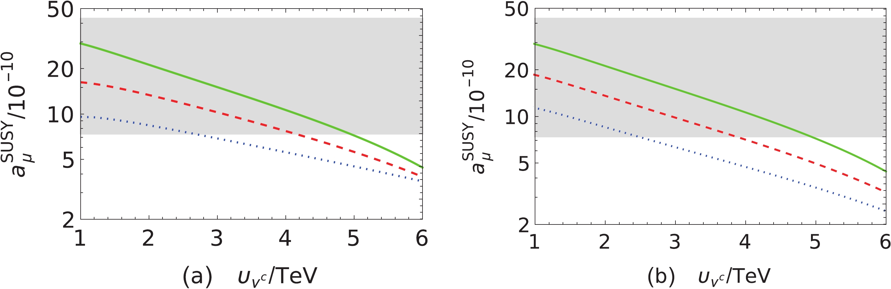
Figure 4. (color online)
$ a_\mu^{\rm{SUSY}} $ versus$ \upsilon_{\nu^c} $ with different$ M_2 $ (a) and$ \tan \beta $ (b), where the gray area denotes$ \Delta a_\mu $ at$ 3.0\sigma $ given in Eq. (1).Through random scanning the parameter space shown in Table 1, we plot the anomalous magnetic dipole moment of muon
$ a_\mu^{\rm{SUSY}} $ varying with the key parameters$ \tan \beta $ (a) and$ \upsilon_{\nu^c} $ (b) in Fig. 5, where the gray area denotes$ \Delta a_\mu $ at$ 3.0\sigma $ given in Eq. (1). Here, the red triangles are excluded by$ \Delta a_\mu $ at$ 3.0\sigma $ . The green points of the$ \mu\nu $ SSM agree with$ \Delta a_\mu $ at$ 3.0\sigma $ , which can explain the current difference between the experimental measurements and the SM theoretical prediction for the muon anomalous MDM.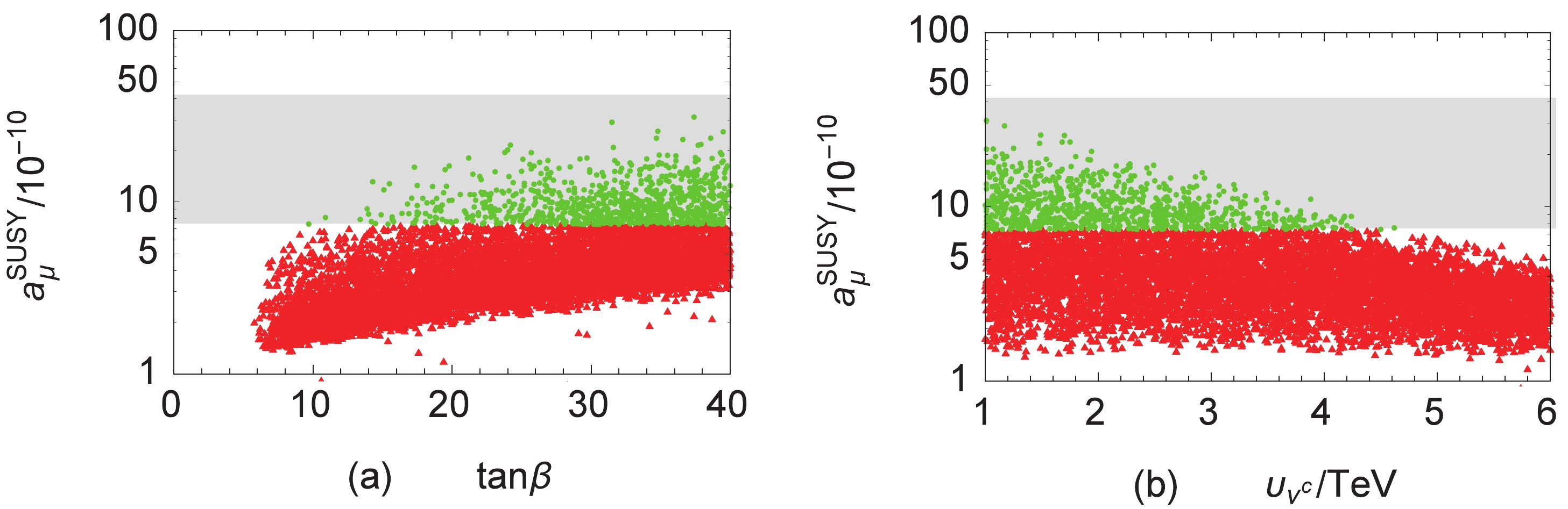
Figure 5. (color online)
$ a_\mu^{\rm{SUSY}} $ versus$ \tan \beta $ (a) and$ \upsilon_{\nu^c} $ (b), where the gray area denotes$ \Delta a_\mu $ at$ 3.0\sigma $ given in Eq. (1) and the red triangles are eliminated.Figure 5(a) shows that the muon anomalous MDM
$ a_\mu^{\rm{SUSY}} $ increases with an increase in the parameter$ \tan \beta $ . One can find that a significant region of the parameter space is excluded by$ \Delta a_\mu $ at$ 3.0\sigma $ in the small$ \tan \beta $ region. Here, the very small$ \tan \beta $ region is also easily eliminated by the constraint of the 125 GeV Higgs boson mass. The numerical results in Fig. 5(b) depict that the muon anomalous MDM$ a_\mu^{\rm{SUSY}} $ is decoupling with increasing$ \upsilon_{\nu^{c}} $ . Therefore,$ \upsilon_{\nu^{c}} $ can affect the masses of charginos and neutralinos. We can see that the value of the muon anomalous MDM$ a_\mu^{\rm{SUSY}} $ in the$ \mu\nu $ SSM could explain the experimental muon anomalous MDM$ \Delta a_{\mu} $ at$ 3.0\sigma $ shown in Eq. (1), when$ \upsilon_{\nu^{c}} $ is small and$ \tan \beta $ is large. Constrained by$ \Delta a_{\mu} $ at$ 3.0\sigma $ shown in Eq. (1),$ \tan \beta<10 $ or$ \upsilon_{\nu^{c}}>5 $ TeV will be easily eliminated.To see more clearly, we plot the anomalous magnetic dipole moment of muon
$ a_\mu^{\rm{SUSY}} $ varying with the lightest chargino mass$ m_{\chi_1} $ in Fig. 6(a), through scanning the parameter space shown in Table 1. The results show that the contribution of the lightest chargino mass$ m_{\chi_1} $ is roughly similar with the contribution of the parameter$ \upsilon_{\nu^c} $ . Because here$ \mu \equiv 3\lambda\upsilon_{\nu^{c}} $ , where μ directly affect the masses of the charginos. In Fig. 6(b),$ a_\mu^{\rm{SUSY}} $ versus$ m_{{{\tilde e}^c}} $ is also pictured. When$ m_{{{\tilde e}^c}} $ is small,$ a_\mu^{\rm{SUSY}} $ in the$ \mu\nu $ SSM could explain the$ \Delta a_{\mu} $ at$ 3.0\sigma $ . The variation trend of$ a_\mu^{\rm{SUSY}} $ versus$ m_{{{\tilde e}^c}} $ coincides with the decoupling theorem; therefore,$ m_{{{\tilde e}^c}} $ directly affects the masses of the slepton. One can see that the anomalous magnetic dipole moment of muon$ a_\mu^{\rm{SUSY}} $ can reach$ \Delta a_{\mu} $ at$ 3.0\sigma $ as shown in Eq. (1), when$ m_{\chi_1}<1.1 $ TeV and$ m_{{{\tilde e}^c}}<1.5 $ TeV.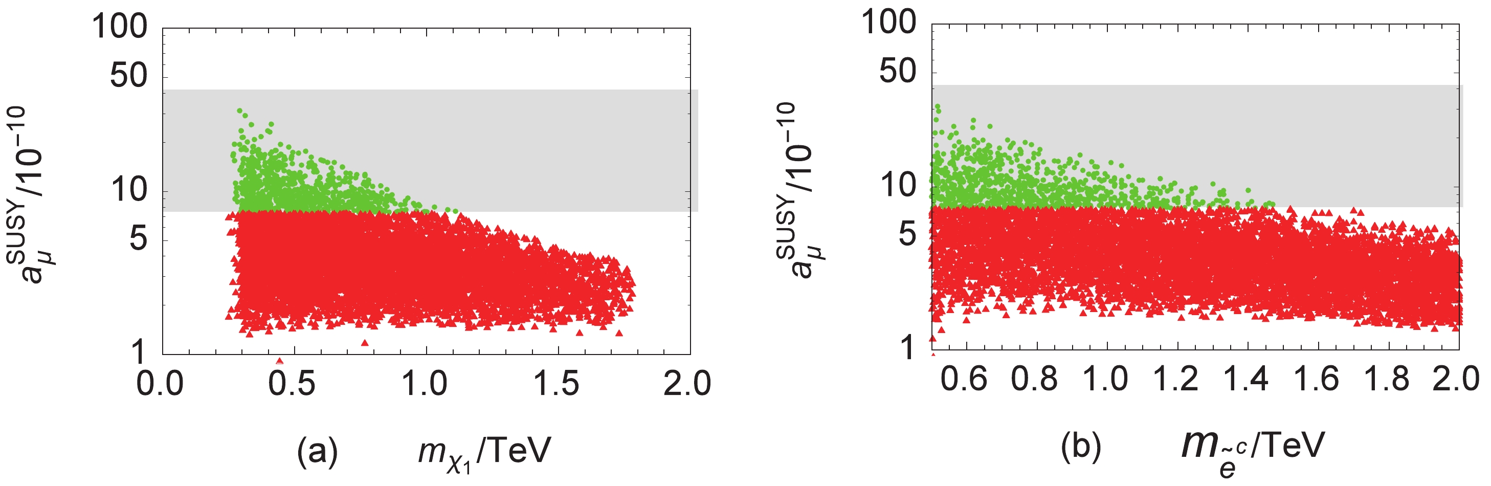
Figure 6. (color online)
$ a_\mu^{\rm{SUSY}} $ versus$ m_{\chi_1} $ (a) and$ m_{{{\tilde e}^c}} $ (b), where the gray area denotes$ \Delta a_\mu $ at$ 3.0\sigma $ given in Eq. (1) and the red triangles are eliminated.For the anomalous MDM of the electron and tau lepton, we also picture
$ a_\mu^{\rm{SUSY}} $ versus$ a_e^{\rm{SUSY}} $ (a) and$ a_\tau^{\rm{SUSY}} $ (b) in Fig. 7, where the green points are in agreement with$ \Delta a_\mu $ at$ 3.0\sigma $ given in Eq. (1) and the red triangles are eliminated by that. Constrained by the updated discrepancy for$ \Delta a_\mu $ at$ 3.0\sigma $ , the anomalous MDM$ a_e^{\rm{SUSY}} $ and$ a_\tau^{\rm{SUSY}} $ in the$ \mu\nu $ SSM are about$ 0.7\times10^{-13} $ and$ 0.8\times10^{-6} $ , respectively. The numerical results show that the ratio between the anomalous MDMs of the tau lepton and muon is about$ 2.8\times10^2 $ , which is in agreement with$ {\bigtriangleup a_\tau}/{\bigtriangleup a_\mu}\simeq m_\tau^2/m_\mu^2\simeq2.8\times10^2 $ . The ratio between the anomalous MDMs of the muon and electron also is consistent with$ {\bigtriangleup a_\mu}/{\bigtriangleup a_e}\simeq m_\mu^2/m_e^2\simeq4.3\times10^4 $ .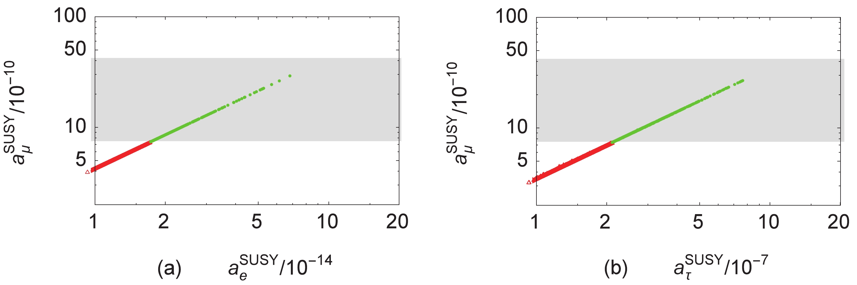
Figure 7. (color online)
$ a_\mu^{\rm{SUSY}} $ versus$ a_e^{\rm{SUSY}} $ (a) and$ a_\tau^{\rm{SUSY}} $ (b), where the gray area denotes$ \Delta a_\mu $ at$ 3.0\sigma $ given in Eq. (1), and the red triangles are eliminated by$ \Delta a_\mu $ at$ 3.0\sigma $ . -
We define the physical quantity
$ \delta_{l_i}\equiv {{\Gamma}_{\rm{NP}}(h\rightarrow {l_i}\bar{{l_i}})-{\Gamma}_{\rm{SM}}(h\rightarrow {l_i}\bar{{l_i}})\over {\Gamma}_{\rm{SM}}(h\rightarrow {l_i}\bar{{l_i}})}, $

(34) to show the difference in the decay width of
$ h\rightarrow {l_i}\bar{{l_i}} $ of the$ \mu\nu $ SSM ($ {\Gamma}_{\rm{NP}}(h\rightarrow {l_i}\bar{{l_i}}) $ ) and that of the SM ($ {\Gamma}_{\rm{SM}}(h\rightarrow {l_i}\bar{{l_i}}) $ ), where$ {l_i}=e,\mu,\tau $ . Firstly, to illustrate clearly the cross-correlation of the model parameters, we plot the ratio$ \delta_\mu $ (a) and$ \delta_\tau $ (b) versus the parameter$ \tan\beta $ with different$ \upsilon_{\nu^c} $ in Fig. 8, taking$ m_{{\tilde L}}=m_{{{\tilde e}^c}}=0.6 $ TeV,$ M_2=2 $ TeV,$ m_{{\tilde u}^c_3}=2 $ TeV and$ A_t=3 $ TeV for simplicity. In Fig. 8, the solid line denotes$ \upsilon_{\nu^c}=6 $ TeV, the dashed line denotes$ \upsilon_{\nu^c}=3 $ TeV, and the dotted line denotes$ \upsilon_{\nu^c}=1 $ TeV. The numerical results in Fig. 8 show that the ratios$ \delta_\mu $ and$ \delta_\tau $ increase with increasing$ \tan\beta $ or$ \upsilon_{\nu^{c}} $ . The charged lepton Yukawa couplings obtain large$ \tan\beta $ enhancements, with$ {Y_{{e_i}}} = {{{m_{{l_i}}\sqrt{\tan^2\beta+1}}}}/{{{\upsilon}}} $ .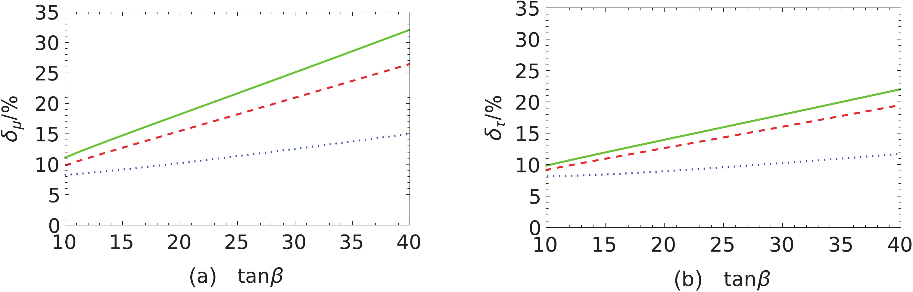
Figure 8. (color online) Ratio
$ \delta_\mu $ (a) and$ \delta_\tau $ (b) versus the parameter$ \tan\beta $ with different$ \upsilon_{\nu^c} $ .Through scanning in Table 1, we plot Figs. 9, 10, where the green dots are the corresponding physical quantity values of the remaining parameters after being constrained by the muon anomalous MDM
$ a_{\mu}^{\rm{SUSY}} $ in the$ \mu\nu $ SSM, with$ 7.4\times 10^{-10} \leq a_{\mu}^{\rm{SUSY}} \leq 42.8\times 10^{-10} $ considered a$ 3 \sigma $ experimental error. The red triangles are ruled out by the muon anomalous MDM with$ a_{\mu}^{\rm{SUSY}}> 42.8\times 10^{-10} $ and$ a_{\mu}^{\rm{SUSY}} < 7.4\times 10^{-10} $ .
Figure 9. (color online) Ratio
$ \delta_\mu $ versus the parameter$ \tan\beta $ (a) and$ \upsilon_{\nu^{c}} $ (b).
Figure 10. (color online) Ratio
$ \delta_\tau $ versus the parameter$ \tan\beta $ (a) and$ \upsilon_{\nu^{c}} $ (b).In Fig. 9, we plot the ratio
$ \delta_\mu $ varying with the parameter$ \tan\beta $ (a) and$ \upsilon_{\nu^{c}} $ (b). We can see that the ratio$ \delta_\mu $ increases with increasing$ \tan\beta $ in Fig. 9(a). The ratio$ \delta_\mu $ can be close to 30$ \% $ when the parameter$ \tan\beta $ is large, constrained by$ \Delta a_\mu $ at$ 3.0\sigma $ . Fig. 9 (b) shows that the ratio$ \delta_\mu $ is non-decoupling with increasing$ \upsilon_{\nu^{c}} $ . The maximum of the ratio$ \delta_\mu $ is around 15$ \% $ as$ \upsilon_{\nu^c} $ is about 1 TeV and close to 30$ \% $ as$ \upsilon_{\nu^c} $ is about 3 TeV. In the$ \mu\nu $ SSM, the parameter$ \upsilon_{\nu^{c}} $ leads to a mixing of the neutral components of the Higgs doublets with the sneutrinos. This mixing affects the lightest Higgs boson mass and the Higgs couplings, which is different in the SM.In addition, we plot the ratio
$ \delta_\tau $ varying with the parameter$ \tan\beta $ and$ \upsilon_{\nu^{c}} $ in Fig. 10, which has a variation trend similar to that of the ratio$ \delta_\mu $ . The numerical results show that, constrained by the experimental value of the muon anomalous MDM, the ratio$ \delta_\tau $ can be about$ 20\% $ when$ \tan \beta $ is about 40 and$ \upsilon_{\nu^c} $ is around 3 TeV. -
Considering that the new experimental average for the muon anomalous MDM increases the difference between the experiments and SM prediction to 4.2σ, we analyze the muon anomalous MDM at the two-loop level in the
$ \mu\nu $ SSM. The numerical results show that the$ \mu\nu $ SSM can explain the current difference between the experimental measurements and the SM theoretical prediction for the muon anomalous MDM, constrained by the 125 GeV Higgs boson mass and decays, the rare decay$ \bar{B}\rightarrow X_s\gamma $ and so on. The new experimental average of the muon anomalous MDM considered that a$ 3 \sigma $ also gives a strict constraint for the parameter space of the$ \mu\nu $ SSM, which constrains that$ \tan \beta>10 $ ,$ m_{{{\tilde e}^c}}<1.5 $ TeV and$ \upsilon_{\nu^{c}}<5 $ TeV with$ \lambda=0.1 $ . Moreover, the anomalous MDM of the tau lepton and the electron in the$ \mu\nu $ SSM can reach about$ 0.7\times10^{-13} $ and$ 0.8\times10^{-6} $ , respectively, constrained by the new experimental average of the muon anomalous MDM at$ 3.0\sigma $ .An upgrade to the Muon g-2 experiment at Fermilab and another experiment at the J-PARC [155] will lead to measurements of the muon anomalous magnetic dipole moment with higher precision, which may reach a 5σ deviation from the SM, constituting an augury for new physics beyond the SM. In addition, the anomalous MDM of the tau lepton and electron, whether deviating from the SM prediction, will be determined more accurately, with the development of experiments in the future.
Considering that the ATLAS and CMS collaborations measured the 125 GeV Higgs boson decay into a pair of muons
$ h\rightarrow \mu \bar{\mu} $ recently, we also investigate the 125 GeV Higgs boson decay$ h\rightarrow \mu \bar{\mu} $ at the one-loop level in the$ \mu\nu $ SSM. Compared with the SM prediction, the decay width of$ h\rightarrow \mu \bar{\mu} $ and$ h\rightarrow \tau \bar{\tau} $ in the$ \mu\nu $ SSM can boost up about 30% and 20%, considering the constraint from the muon anomalous magnetic dipole moment. In the$ \mu\nu $ SSM, the mixing of the neutral components of the Higgs doublets with the sneutrinos affects the lightest Higgs boson mass and the Higgs couplings, which can contribute to Higgs boson decay. In the future, high luminosity or high energy large colliders [156−159] will detect the Higgs boson decay$ h\rightarrow \mu \bar{\mu} $ and$ h\rightarrow \tau \bar{\tau} $ with high precision, which may be an indication for new physics.
Muon anomalous magnetic dipole moment in the μνSSM
- Received Date: 2022-02-16
- Available Online: 2022-09-15
Abstract: Recently, the Muon g-2 experiment at Fermilab measured the muon anomalous magnetic dipole moment (MDM),


 DownLoad: