


 Abstract
 HTML
HTML Reference
 Related
 PDF
PDF


-
The standard cosmological model (ΛCDM) successfully describes the large scale structure evolution of our universe. The main matter component in the ΛCDM, called dark matter (DM), which is yet to be detected, is one of the most outstanding puzzles in contemporary physics. The cosmology observation accuracy about DM abundance has reached the percent level [1]. The relic abundance of DM needs to be considered beyond the perturbation calculation.
Weakly Interacting Massive Particle (WIMP) [2] is one of the most popular dark matter candidates. In the standard paradigm, the relic abundance of WIMP dark matter is usually given by the thermal freeze-out mechanism [3, 4]. If there exists a long-range force between two non-relativistic moving particles, non-perturbation effect needs to be considered. This effect can be calculated by the ladder diagram in Quantum Field Theory [5]. It can also be approximately calculated by quantum mechanics, considering that the two particle pair wave function is modified by the long-range force. The DM particles are non-relativistic during freeze-out in most models about WIMP (so we called it cold dark matter). Many studies focus on the non-perturbation effects of annihilation particles, for example, the Sommerfeld effect and bound state effect①.
Previous works about the bound state effect focused on the initial DM or co-annihilator pairs [5–18]. However, when annihilation products have coupling with a light force mediator, and have been mass-degenerate with the initial DM, non-perturbation effects also occur in final state particles. In the early universe, the initial annihilating particle energy obeys the Maxwell-Boltzmann distribution. Therefore, they can have enough energy to annihilate into heavier particles (Forbidden DM [19] or Impeded DM [20]). Recently, the final state Sommerfeld effect (FSS) has been considered in the DM relic abundance calculation [21]. It is showed that the s-wave FSS has a significant influence on the DM relic abundance. We naturally extend to study the p-wave FSS effect in this work.
In fact, the FBS formation has been discussed routinely in the Standard Model (SM), including
$ e^+e^-\rightarrow (\mu^+\mu^-) $ [22] and$ q\bar{q}\rightarrow (\mu^+\mu^-)g $ [23], where the bound states are formed by exchanging SM gauge bosons.Usually, the leading FBS formation should be the
$ 2 \to 1 $ process (two dark matter particles annihilate into FBS without emission). But the sub-leading process (two dark matter particles annihilate into FBS with emission) may not be negligible because the leading process cannot always happen when the incoming particle's energy is larger than the mass of the FBS. Another reason is that the sub-leading process can form an s-wave FBS, while the leading process can merely form a p-wave bound state. We provide Model II to illustrate this situation in Sec. IV.FBS can arise due to non-confining forces (hydrogen and positronium) or confining forces (hadronic bound states) [24]. Another class of bound states, non-topological solitons, has also been considered in the context of DM [25, 26]. Here, we consider FBS formed due to non-confining interactions and calculate the cross sections for FBS formation in the non-relativistic regime, which is relevant for cosmology and DM indirect detection signals. If the FBS can exist as a portal between DM sectors and SM particles, it has the possibility to provide new detectable signals. For instance, the FBS has different energy levels. Like hydrogen, its decay and transition give the spectrum of SM particles. For example, an FBS formed due to a dark photon exchange, which has kinetic mixing with the photon [27, 28].
The rest of our paper is organized as follows. In Sec. II, we introduce the FBS formation conditions and assumptions and provide a physical depiction of the FBS. In Secs. II.B and II.C, we show the paradigm of calculating the DM relic abundance with FBS and FSS effects in the thermal freeze-out scenario. Sec. III presents the analytical calculation about the cross sections for the DM Model I, the numerical results about thermal-averaged cross sections, FBS effect on DM relic abundance, and a brief discussion on the results. Sec. IV is the same as Sec. III, but for the DM Model II. DM Model II is proposed to demonstrate the difference from Model I when considering the conservation of angular momentum. The Models, both show that the FBS can have an important effect on relic abundance. Finally, in Sec. V, we summarize our conclusions.
-
When the annihilation products are non-relativistic and have a coupling with a light force mediator, a bound state can form between final products. For simplicity, we consider the scenario where two dark matter particles annihilate into two final state particles; the two final particles form a bound state, and the excessive energy of incoming particles is carried away by emitting a vector boson. This process can be described by Fig. 1.
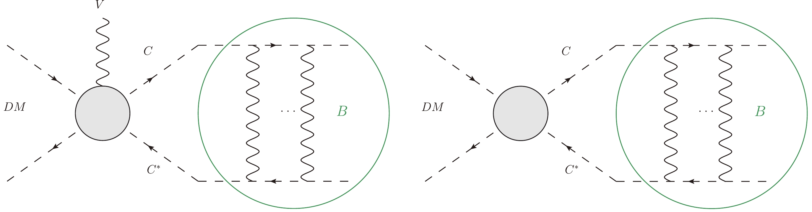
Figure 1. (color online) Feynman diagram for an FBS formation. The two pictures both describe two incoming DM particles that annihilate into an FBS, which is formed by a
$ CC^* $ pair. The difference between the two panels: in the left panel, the incoming DM energy exceeds the FBS mass, and the extra energy is carried away by a vector boson; in the right panel, the incoming DM energy equals the FBS mass.It is not difficult to understand the FBS formation using the analogy of positronium or true muonium formation [22, 29, 30]. The FBS has different energy levels like positronium, the most contributive channel is the s-wave FBS formation, and then the p-wave FBS formation. Considering the selection rule, in some situations, the s-wave channel cannot occur, it can only start from a p-wave channel. We propose Moldel II in Sec. IV to demonstrate the situation in which FBS formation can only start from a p-wave channel.
Another point is about the FBS lifetime. In this work, the FBS formed due to the non-relativistic final state particles exchange with the Abelian light mediator, just like the positronium and true muonium. They are not in a stable state and finally dissociate or decay, but it does not matter in our calculation. The final particles are regarded as a portal between the DM sector and SM sector; they finally decay into an SM particle and fade out as universe cools down. However, when the DM freezes-out, they are still deemed to be within the thermal bath of SM particles. We assume the annihilation products have strong enough couplings, directly or indirectly, with SM particles, so that the C and the SM particles can maintain kinetic equilibrium and have the same temperature during the dark matter freeze-out. If C couples with the SM particles via a dark photon, V, the coupling ,
$ \alpha_{V} $ , we considered is large enough ($ \alpha_{V}=0.02 $ is already sufficiently large) for this assumption to be valid [8, 31]. The final state particle, C (and$ C^* $ ), may decay into other lighter particles, which carry the same$ U(1) $ charge. Therefore, the current experimental bounds on the dark photon parameters may not be directly translated to the bounds on$ \alpha_{V} $ and$ m_C $ . On the other hand, it is possible to let the$ CC^* $ particle's annihilation cross section be sufficiently large, so that C and$ C^* $ can maintain thermal equilibrium during DM freeze-out. We only use the assumption that the final state particles are in thermal equilibrium during DM freeze-out, and building a full model is beyond the scope of this work. So, we can use the simple Maxwell-Boltzmann distribution for them when we calculate the DM relic abundance. FBS exists as a portal and also brings many interesting DM indirect detection signals [27, 28, 32], but we will not discuss this here. Next we briefly explain why the existence of FBS will influence the DM relic abundance.First, during freeze-out, most of the DM particles are moving with non-relativistic velocities. As the annihilation products of DM, the final state particles are naturally non-relativistic when their masses are degenerate with DM. As mentioned above, if the final state particles can exchange a light vector boson, or in non-relativistic approximation, exits a long range force, and the revolution time is smaller than the lifetime of the FBS components [33], it can form an FBS.
Second, in the early universe, SM particles and DM particles coupling with the SM are all in a thermal bath. The velocity of the particles in the thermal bath can be approximately described by the Maxwell-Boltzmann distribution. Therefore, there are always DM particles with enough energy that can annihilate into heavier particles [19, 20, 34]. In this case, the FBS formation processes are permitted even if the final state particles have larger mass than the DM. The "forbidden" cases are considered more significant because the FBS formation without emission can happen. In such instances, we naturally study the FBS effect on the DM relic abundance.
-
To calculate the FBS or FSS effects on DM relic abundance, we need to average the cross sections over the momentum distribution of DM in the early universe. All the initial and final particles are in the plasma, the Maxwell-Boltzmann distribution is parameterized by the energy of DM particles
$ \begin{array}{*{20}{l}} f(E)\propto {\rm e}^{-{(Ex)}/{m_D}}, \end{array} $

(1) where
$ x\equiv m_D/T $ ,$ m_D $ is the DM mass, and E is the energy of DM particle. The thermal-averaged cross section times relative velocity of DM annihilation are given by$ \langle \sigma v\rangle =\frac{\int\sigma v{\rm e}^{-{(E_1x)}/{m_D}}{\rm e}^{-{(E_2x)}/{m_D}}{\rm d}^3{\boldsymbol{p}}_1{\rm d}^3{\boldsymbol{p}}_2}{\int {\rm e}^{-{(E_1x)}/{m_D}}{\rm e}^{-{(E_2x)}/{m_D}}{\rm d}^3{\boldsymbol{p}}_1{\rm d}^3{\boldsymbol{p}}_2}. $

(2) By changing the integration variables, the thermal-averaged cross section finally can be expressed as [35]
$ \langle \sigma v\rangle=\frac{1}{8m_D^4TK_2^2(m_D/T)}\int_{s_{\rm min}}^\infty\sigma(s-4m_D^2)\sqrt{s}K_1(\sqrt{s}/T){\rm d}s, $

(3) where
$ s=(p_1+p_2)^2 $ is the Mandelstam variable and$ K_i $ is the modified Bessel functions of order i. The integral must be from$ s_{\rm min} $ , rather than$ 4m_D^2 $ to take into account the threshold mentioned above. -
In this section we discuss the relic abundance calculation, including FBS formation. We assume a simple condition that the annihilation products quickly thermalize and their number densities equal the thermal equilibrium values, as we mentioned in Sec. II. Therefore, only
$ one $ Boltzmann equation is needed to calculate the DM$ yield $ , which is the ratio of the DM density to the entropy density,$ Y\equiv n/s $ . The Boltzmann equation can be written as$ \frac{{\rm d}Y_D}{{\rm d}x}=-\frac{xs}{H(m_D)}\left(1+\frac{T}{3g_{*s}}\frac{{\rm d}g_{*s}}{{\rm d}T}\right)\langle \sigma v\rangle(Y_D^2-Y_{Deq}^2). $

(4) Noting that:
$ \begin{aligned}[b] n_{eq}=&\frac{T}{2\pi^2}gm_D^2K_2(x),\quad s=\frac{2\pi^2}{45}g_{*s}m_D^3/x^3, \\ & H(m_D)= \left(\frac{4\pi^3G_Ng_*}{45}\right)^{{1}/{2}}m_D^2, \end{aligned} $

(5) where g is the DM degrees of freedom;
$ K_2(x) $ is the modified Bessel function of the second kind;$ G_N $ is the gravitational constant;$ H(T) $ is the Hubble parameter; and$ g_{*s} $ and$ g_* $ are the numbers of effectively massless degrees of freedom associated with the entropy density and the energy density, respectively.The total thermal-averaged cross section of different channels/effects is
$ \begin{array}{*{20}{l}} \langle\sigma v\rangle_{\rm all}=\langle\sigma v\rangle_{\rm FSS}+\langle\sigma v \rangle_{B}+\langle\sigma v \rangle_{BV}, \end{array} $

(6) where
$ \langle\sigma v\rangle_{\rm FSS} $ ,$ \langle\sigma v \rangle_{B} $ , and$ \langle\sigma v \rangle_{BV} $ are the thermal-averaged cross sections for FSS-corrected annihilation, FBS formation without boson emission, and FBS formation with boson emission, respectively. We just need to put the total thermal cross section,$ \langle\sigma v\rangle_{\rm all} $ , into Boltzmann Eq. (4) and then solve the$ yield $ with the FSS and FBS formation effects. The DM relic abundance is given by$ \Omega_D h^2= 2.755 \times 10^8 \frac{m_D}{\rm GeV}Y_{D,0}, $

(7) where h is the present-day dimensionless Hubble parameter;
$ Y_{D,0} $ is the DM$ yield $ solved by the Boltzmann equation and taking the value at the limit$ x \to \infty $ . -
In this section, we employ a simple scalar QED-like model, which carries the light force mediator, to illustrate the FBS formation effect and FSS effect on relic abundance. We will calculate the cross section of FBS formation, and the cross section of the channel with the FSS effect according to the model. Then, we follow the process in Sec. II and give the numerical results.
In this model, we consider DM consisting of a real scalar particle, D, coupled to a complex scalar particle, C, via a four-point interaction. As a DM annihilation product, C also has QED-like couplings with a light, real vector boson, V (for example, a dark photon). The model is summarized by the Lagrangian:
$ \mathcal{L}_I\supset|D_\mu C|^2+\frac{1}{2}g_DD^2|C|^2, $

(8) where
$D_\mu=\partial_\mu-{\rm i}g_VV_\mu$ is the covariant derivative. The coupling constant of the four-point interaction is$ {g}_D $ . The$ V_\mu $ stands for the light, real vector boson.In
$ zero $ temperature, the vector boson mass is$ zero $ . While, in the thermal bath, the Coulomb force gets screened by the thermal plasma. This can be described by a vector Debye mass [36, 37]:$ \begin{array}{*{20}{l}} m_V\sim g_VT, \end{array} $

(9) where T is the thermal bath temperature. The incoming DM particles, D, with mass
$ m_D $ and the outgoing particles, C, with mass$ m_C $ . We assume that the vector boson mass all comes from the Debye mass. However, in calculating the FSS and FBS effects, we still use a Coulomb-like potential since DM freeze-out happens at a temperature much smaller than the DM mass (typically$ T_{\rm freeze-out}\thicksim m_D/25 $ ). The Debye mass is scanning when temperature decreases, so the Sommerfeld factor,$ S_ f $ , has resonant behavior [31]. However, the difference between the thermal-averaged FSS-corrected cross sections is within several percent when we use the Coulomb-like potential and the Hulthen potential (which is a good approximation for the Yukawa potential). Therefore, during and after freeze-out, a Coulomb-like potential is a good approximation. -
In this model, the DM particle, D, can directly annihilate into C via four-point interaction, as shown in Fig. 2. The amplitude for this process is
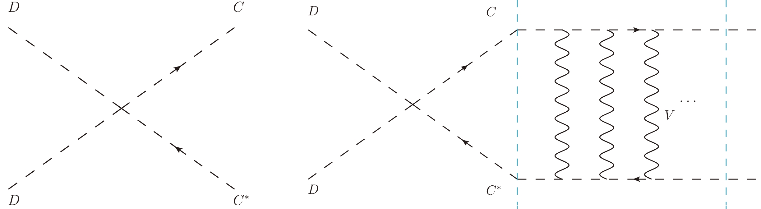
Figure 2. (color online) Feynman diagrams for
$ DD\rightarrow CC^* $ annihilation without/with the FSS effect.$ \begin{array}{*{20}{l}} {\rm i}{\mathcal{M}}_{DD\rightarrow CC^*} =-{\rm i}g_D. \end{array} $

(10) The cross section times relative velocity, v, of the incoming DM particles in the (center-of-momentum) COM frame is
$ \begin{aligned}[b] & (\sigma _{ann} v) = \frac{g_D^2}{8\pi s}v_2, \\ & v_2=\sqrt{1-4m_C^2/s}, \end{aligned} $

(11) where
$ s=(p_1+p_2)^2 $ is the Mandelstam variable, and$ v_2 $ is the velocity of final state particle, C, in COM. It is the part under the square root that has to be greater than$ zero $ for the "forbidden" case. We can directly calculate$ s_{\rm min} $ by setting it equal to$ zero $ for the "forbidden" case. Therefore, when$ m_C>m_D $ ,$ s_{\rm min} = 4 m_C ^2 $ ; otherwise,$ s_{\rm min} = 4 m_D ^2 $ .Since the final state particle, C, has a coupling with V, we shall consider a simple Coulomb-like potential between the final
$ CC^\ast $ pair in non-relativistic terms. The consequence is the FSS effect. This effect has been previously considered in [21]. Because the matrix element is a constant here, there is only the s-wave Sommerfeld effect. Multiplying by the s-wave Sommerfeld factor, the cross section takes the form of$ \begin{aligned}[b] & (\sigma v)_{\rm FSS} = (\sigma _{ann} v) \ S_ f \,,\\ & {S_ f}=\frac{\pi\alpha_{V}/v_2}{1-{\rm e}^{-\pi\alpha_{V}/v_2}}, \quad \alpha_{V} = \frac{g_V ^2}{4 \pi}, \end{aligned} $

(12) where
$ S_ f $ is the FSS factor for s-wave annihilation.For the FSS effect, since
$ S_ f $ is applicable to a non-relativistic final state velocity, we choose to turn off the FSS effect for$ v_2>0.6 $ . In the following calculation, we substitute$ S_ f $ with$[(S_{ f}-1)H(0.6-v_2)+ 1]$ , where$ H(0.6-v_2) $ is the Heaviside step function following the treatment in [21].After calculating the cross section and the
$ s_{\rm min} $ , one can follow the process in Sec. II.B to work out the thermal-averaged$ \langle\sigma v\rangle_{\rm FSS} $ . -
C and
$ C^* $ can bind into positronium-like states; the s-wave (orbital angular momentum$ L=0 $ ) FBS can be allowed to form. Fig. 3 shows this process.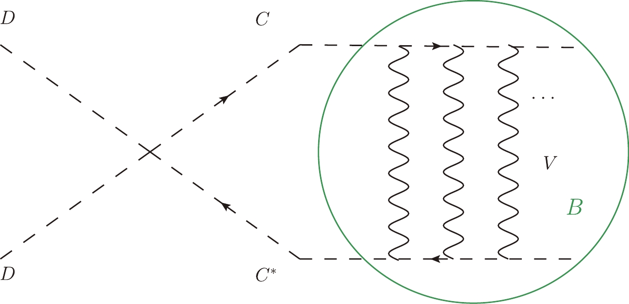
Figure 3. (color online) The Feynman diagram for
$ DD^\ast \rightarrow B $ annihilation.The scattering amplitude of this process considering the ground bound state formation is
$ \mathcal{M} _{DD \rightarrow B(L=0)} = \sqrt{\frac{1}{m_C}}\int \frac{{\rm d}^3{\boldsymbol{k}}}{(2\pi)^3} \widetilde{\psi}_{n00} ^*({\boldsymbol{k}})\mathcal{M}_{DD\rightarrow CC^*}, $

(13) where
$ \widetilde{\psi} $ is the wave function in momentum space. Because the matrix element for$ DD\rightarrow CC^* $ does not depend on$ {\boldsymbol{k}} $ , we can directly use the relation$ \int\frac{{\rm d}^3{\boldsymbol{k}}}{(2\pi)^3}\widetilde{\psi}^*_{n00} ({\boldsymbol{k}})=\psi^*_{n00} ({\boldsymbol{r}}=0), $

(14) where
$ \psi^*_{n00}({\boldsymbol{r}}=0)=\frac{1}{\sqrt{\pi}(na_0)^{3/2}} $

(15) is the s-wave hydrogen-like wave function for the
$ CC^* $ bound state, where$ a_0=1/(\mu\alpha_{V}) $ is the Bohr radius, and the mass is reduced to$ \mu=m_C/2 $ . We denote this process as$ DD\rightarrow B(L=0) $ , and work in the COM frame to obtain$ |\mathcal{M}_{DD\rightarrow B(L=0)}|^2=\frac{g_D^2\alpha_{V}^3m_C^2}{8n^3\pi}. $

(16) The cross section times relative velocity is [38]
$ (\sigma v)_B = \frac{2\pi}{s}|\mathcal{M} _{DD\rightarrow B(L=0)}|^2 \ \delta \left(E_{\rm cm}^2-m_B^2\right), $

(17) where
$ m_B=2m_C-E_B=2m_c-\dfrac{\alpha_{V}^2m_C}{4n^2} $ and is the bound state mass,$ E_B $ is the binding energy, and the δ function ensures energy-momentum conservation. Again, the thermal-averaged cross section,$ \langle\sigma v \rangle_{DD\rightarrow B} $ , can be worked out according to Sec. II.B.In the numerical calculation, we only include
$ n=1,\;L=0 $ in the FBS. It is also possible to form an FBS with a principal quantum number larger than$ 1 $ , corresponding to$ \widetilde{\psi}^*_{n00} ({\boldsymbol{k}}) $ ; the result provides the amount to multiply by a factor$ {1}/{n^3} $ to$ \psi^*_{100}({\boldsymbol{r}}=0) $ . The total contribution for these excited bound states will enlarge the result of FBS formation without the emission by a factor on the order of$ 1 $ . We neglect those contributions in this work, and therefore, our result is conservative. For other cross sections in Model I and Model II, we still only consider the relevant smallest principal quantum number. -
A bound state can also form via a vector boson emission process as shown in Fig. 4. First of all, noting that a vector boson carries a spin of one, the first term allowed is the p-wave (orbital angular momentum
$ L=1 $ ) FBS.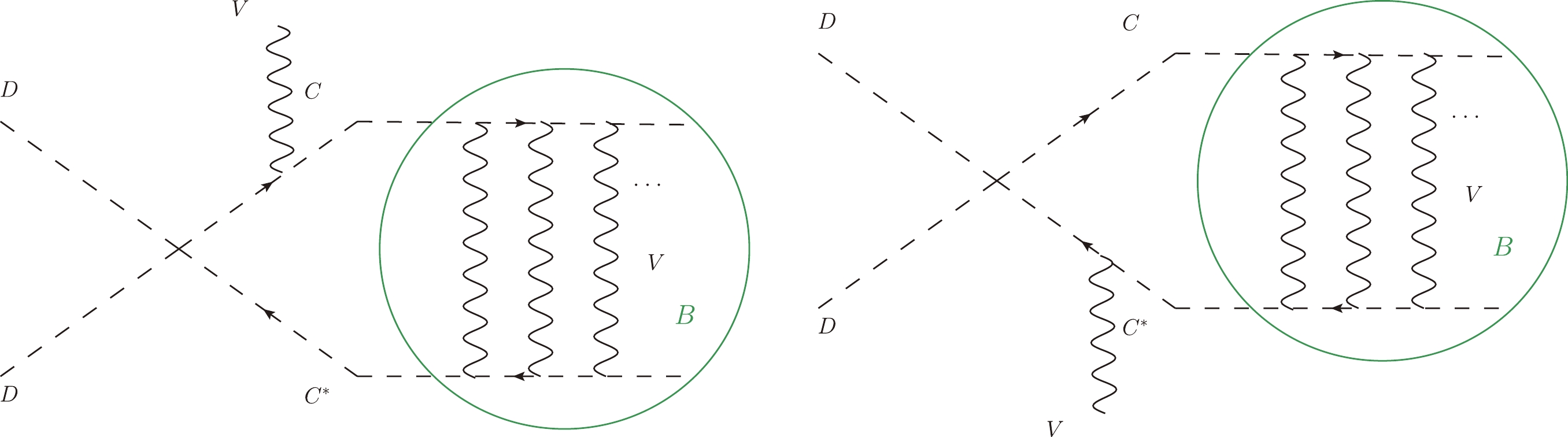
Figure 4. (color online) The Feynman diagrams for the
$ (CC^*) $ bound state production process$ DD\rightarrow BV $ .The scattering amplitude for the process
$ DD\rightarrow CC^*V $ can be written as$ \begin{aligned}[b] {\rm i}\mathcal{M}_{DD\rightarrow CC^*V} =& {\rm i}g_Dg_V\Bigg(\frac{2k_2\cdot \epsilon^*(q)+q\cdot\epsilon^*(q)}{2k_2\cdot q+m_V^2}\\&-\frac{2k_1\cdot \epsilon^*(q)+q\cdot\epsilon^*(q)}{2k_1\cdot q+m_V^2}\Bigg)\,, \end{aligned} $

(18) where
$ p_1 $ ,$ p_2 $ ,$ k_1 $ ,$ k_2 $ , and q are, respectively, the momenta of D, D, C,$ C^* $ and V.$ \epsilon _\mu $ is the vector boson, V, polarization vector satisfying$ \sum\limits_{\lambda =1}^{3}\epsilon_\mu (q)\epsilon_\nu (q)=-g_{\mu\nu}+\frac{q_\mu q_\nu}{m_V^2}. $

(19) We introduce the total and relative momenta,
$ {\boldsymbol{K}}={\boldsymbol{k_1}}+ {\boldsymbol{k_2}} $ and$ {\boldsymbol{k}}=({\boldsymbol{k_1}}-{\boldsymbol{k_2}})/2 $ , for C and$ C^* $ . In the bound state rest frame,$ {\boldsymbol{K}}=0 $ . It allows us to rewrite Eq. (18) under the non-relativistic approximation and expand to the first order of$ {\boldsymbol{k}} $ , as$ \mathcal{M}^j_{DD\rightarrow CC^*V}\simeq -g_Dg_V\left(\frac{4k^j}{2m_C\omega +m_V^2}+\frac{4q^j({\boldsymbol{k}}\cdot{\boldsymbol{q}})}{(2m_C\omega+m_V^2)^2}\right), $

(20) where ω is the vector boson energy and index j stands for the spatial 3-components.
The products of
$ DD $ can form bound states. We write the amplitude$ \mathcal{M}_{DD\rightarrow BV} $ in terms of the final$ CC^* $ pair momentum$ {\boldsymbol{K}} $ and$ {\boldsymbol{k}} $ . The FBS effect can be calculated as follows: the matrix element multiplies the momentum space wave function ($ L=1 $ ), integrating out the relative momentum,$ {\boldsymbol{k}} $ [5, 38].$ \begin{array}{*{20}{l}} \begin{aligned} \mathcal{M}^j_{BV}=\sqrt{\frac{1}{m_C}}\int \frac{{\rm d}^3{\boldsymbol{k}}}{(2\pi)^3}\widetilde{\psi}_{21m} ^*({\boldsymbol{k}}) \ \mathcal{M}^j_{DD\rightarrow CC^*V}\,. \end{aligned} \end{array} $

(21) A mathematical trick can be used in the integrals with respect to
$ {\boldsymbol{k}} $ :$ \int \frac{{\rm d}^3{\boldsymbol{k}}}{(2\pi)^3} k^j \widetilde{\psi} ^{*i}({\boldsymbol{k}})=-{\rm i}\nabla^j\psi ^i({\boldsymbol{x}})|_{{\boldsymbol{x}}=0}\,. $

(22) The value of the
$ L=1 $ wave function at$ {\boldsymbol{r}}=0 $ is$ zero $ . It is clear that the bound state formation matrix elements are proportional to the value of the first-order derivative of the$ L=1 $ wave function at$ {\boldsymbol{r}}=0 $ . The details to deal with a p-wave bound-state can be seen more in [39, 40]. The hydrogen-like wave function of the$ CC^* $ bound-state has the form$ \begin{aligned}[b] \psi _{nlm}({\boldsymbol{r}})=&\left[\frac{1}{2n}\left(\frac{2}{na_0}\right)^3\frac{(n-l-1)!}{(n+l)!}\right]^{1/2}\left(\frac{2r}{na_0}\right)^l\\&\times\mathrm{e}^{-r/na_0}L^{2l+1}_{n-l-1}\left(\frac{2r}{na_0}\right)Y_{lm}(\theta ,\phi ), \end{aligned} $

(23) and
$ L^m_n(x)=(n+m)!\sum\limits_{k = 0}^{n}\frac{(-1)^k}{k!(n-k)!(k+m)!}x^k, $

(24) are the associated Laguerre polynomials.
For the polarization summation of a vector boson, we can follow the method in [41],
$ \begin{aligned}[b] \sum_{m,\lambda}|\mathcal{M}_{DD\rightarrow B(L=1)V}|^2&=\left(-g_{\mu\nu}+\frac{q_\mu q_\nu}{m_V^2}\right)\mathcal{M}^\mu\mathcal{M}^{\nu*}\\ &=\mathcal{M}^j\mathcal{M}^{j*}-\frac{|q^j\mathcal{M}^j|^2}{{\boldsymbol{q}}^2+m_V^2}. \end{aligned} $

(25) Notice that
$ q_\mu\mathcal{M}^\mu=0 $ . Therefore, the formula is the same for massive and massless vector bosons.The final result after the polarization summation is
$ \sum\limits_{m,\lambda}|\mathcal{M}_{DD\rightarrow B(L=1)V}|^2=C\left[\left(3-B\right)+2A\left(1-B\right)+A^2\left(1-B\right)\right], $

(26) where
$ \begin{aligned}[b] A=&\frac{|{\boldsymbol{q}}|^2}{2m_C\omega+m_V^2}=\frac{\omega^2-m_V^2}{2m_C\omega+m_V^2},\\ B=&\frac{|{\boldsymbol{q}}|^2}{|{\boldsymbol{q}}|^2+m_V^2},\\ C=&\frac{g_D^2}{6}\frac{n^2-1}{n^5}\alpha_{V}^6 \frac{4m_C^4}{(2m_C\omega+m_V^2)^2}. \end{aligned} $

(27) In the bound state rest frame, the emission vector boson energy, ω, and 3-momentum modulus square are already fixed by the Mandelstam variable, s, and the masses of particles,
$ \begin{aligned}[b] \omega = \frac{s-m_B^2-m_V^2}{2m_B}, \quad |{\boldsymbol{q}}|^2 = \omega^2 - m_V^2. \end{aligned} $

(28) It is obvious that the boson momentum
$ |{\boldsymbol{q}}| $ must be larger than$ zero $ , it decides the$ s_{\rm min} $ . In the low temperature limit,$ m_V \sim g T = 0 $ , only the first term in the square brackets is left in Eq. (26)$ \sum\limits_{m,\lambda}|\mathcal{M}_{DD\rightarrow B(L=1)V}|^2= \frac{g_D^2}{3}\frac{n^2-1}{n^5}\alpha_{V}^6 \left(\frac{m_C}{\omega}\right)^2. $

(29) There is a pole when the energy of the vector boson
$ \omega=0 $ , which is the usual infrared divergence for soft bremsstrahlung. We can address this problem by introducing a Debye mass, as Eq. (9) shows. In order to take care of this infrared divergence appropriately, we need loop diagrams to offset it.Because the
$ |\mathcal{M}|^2 $ is a Lorentz invariant, for simplicity, we change the reference frame to the COM frame for phase space integration according to the general formula [38]. The cross section times relative velocity, v, of the incoming DM particles for the process$ DD\rightarrow B(L=1)V $ gives$ \begin{aligned}[b] (\sigma v)_{BV}=&\frac{\sum_{m,\lambda}|\mathcal{M}_{DD\rightarrow B(L=1)V}|^2}{4 \pi s } \frac{|{\boldsymbol{q}}|_{\rm cm}}{\sqrt{s}}, \\ |{\boldsymbol{q}}|_{\rm cm} =& \sqrt{\left(\frac{s+m_B^2-m_V^2}{2\sqrt{s}}\right)^2-m_B^2}\,. \end{aligned} $

(30) -
In order to show the BSF formation effects in the non-relativistic region, we plot the thermal-averaged cross sections at three parameters,
$ \alpha_{V} = 0.02, \;0.1, \;0.5 $ , which represent electroweak-like, strong-like, and "super" strong-like coupling, respectively. To explore the FBS effect in the non-relativistic region of final products, we fix the mass of annihilated DM and normalize other particles' mass by it. We use z as the ratio of product particle mass and DM mass,$ z\equiv m_C/m_D $ , and then, we plot the thermal-averaged cross sections evolution as a function of x at three parameters$ z = 0.9, \;1,\; 1.1 $ . -
The cross sections and kinematic threshold
$ s_{\rm min} $ , for three processes are summarized in Table. 1. In the numerical calculation, we only consider$ n=1 $ for the$ DD\rightarrow B $ and$ n=2 $ for the$ DD\rightarrow BV $ .${\rm channel}$ 

$ (\sigma v) $ 

$s_{\rm min}$ 

$ DD\rightarrow CC^* $ 

$\dfrac{g_D^2}{8\pi s}v_2\dfrac{\pi\alpha_{V}/v_2}{1-{\rm e}^{-\pi\alpha_{V}/v_2} }$ 

${\rm Max}[4 m_D^2,4m_C^2]$ 

$ DD\rightarrow B $ 

$\dfrac{g_D^2\alpha_{V}^3m_C^2}{4s}\delta(E_{\rm cm}^2-m_B^2)$ 

$ 4 m_D^2 $ 

$ DD\rightarrow BV $ 

$\dfrac{|{\boldsymbol{q} }|_{\rm cm} }{\sqrt{s} } \ C\left[\left(3-B\right)+2A\left(1-B\right)+A^2\left(1-B\right)\right]/(4\pi s)$ 

${\rm Max}[4 m_D^2, \ (m_B+m_V)^2]$ 

Table 1. Cross sections and kinematically forbidden limits for Model I.
We can directly calculate the thermal-averaged cross sections following Eq. (3) in Sec. II.B. Fig. 5 shows the thermal-averaged cross sections. We choose three values of
$ \alpha_{V} $ ,$ 0.02 $ ,$ 0.1 $ and$ 0.5 $ for illustration, indicating electroweak-like, strong-like, and "super" strong-like couplings, respectively. The red, green, blue, and black lines stand for$ \langle\sigma v\rangle_{\rm FSS} $ ,$ \langle\sigma v \rangle_{B} $ ,$ \langle\sigma v \rangle_{BV} $ , and$ \langle\sigma v \rangle_{\rm w/o \ both} $ over a common fator,$ g_D ^2 / m_D ^2 $ , respectively, as functions of z at a typical freeze-out value,$ x=25 $ . The subscript "w/o both" indicates that both FSS and FBS effects are not included.
Figure 5. (color online) The thermal-averaged cross sections over a common factor,
$ g_D ^2 / m_D ^2 $ , at three parameters,$\alpha_{V} = 0.02,\; 0.1,\; 0.5$ , at a typical freeze-out value,$ x=m_D/T=25 $ . The red, green, blue, and black lines stand for$ \langle\sigma v\rangle_{\rm FSS} $ , the thermal-averaged FSS-corrected s-wave cross section;$ \langle\sigma v \rangle_{B} $ , the thermal-averaged s-wave FBS (without boson emission) formation cross section;$ \langle\sigma v \rangle_{BV} $ , the thermal-averaged p-wave FBS (with boson emission) formation cross section; and$ \langle\sigma v \rangle_{\rm w/o \ both} $ , the thermal-averaged cross section without any FSS and FBS, respectively. z is the mass ratio,$ m_C/m_D $ . The y-axis is the thermal-averaged cross sections divided by a common factor.For a given
$ \alpha_{V} $ , the$ \langle\sigma v\rangle_{B} $ gives much more contribution than$ \langle\sigma v\rangle_{BV} $ because in Model I,$ \langle\sigma v\rangle_{BV} $ corresponding to a p-wave FBS formation is suppressed by$ \alpha_{V}^3 $ (two from the square of wave function and one from interaction vertex). When$ z>1 $ , a single s-wave bound state can be formed② without a vector boson emission. Therefore,$ \langle\sigma v\rangle_{B} $ becomes comparable with$ \langle\sigma v\rangle_{\rm FSS} $ for large$ \alpha_{V} $ . In Fig. 5, as$ \alpha_{V} $ increases from left to right, the binding energy of the FBS increases, meaning it is easier to form a bound state and the bound state gets tighter. The FSS effect also increases because the same light mediator mediates the long range force.The different partial wave FSS/FBS effect is sensitive to the order of
$ \alpha_{V} $ . From the above figure, we can read out the difference of partial wave contributions, and these partial wave FSS/FBS effect relative contributions also change significantly as the$ \alpha_{V} $ value changes.Figure 6 shows the thermal-averaged cross section evolution as temperature cools down. The absence of
$ \langle\sigma v \rangle_{B} $ in the left and the middle panel is because the initial energy in$ z=0.9 $ and$ z=1 $ is always larger than the single bound state energy. The rest mass of forming a bound state must be released by emitting a vector boson; hence, the FBS effect is only contributed by the$ DD \to BV $ process.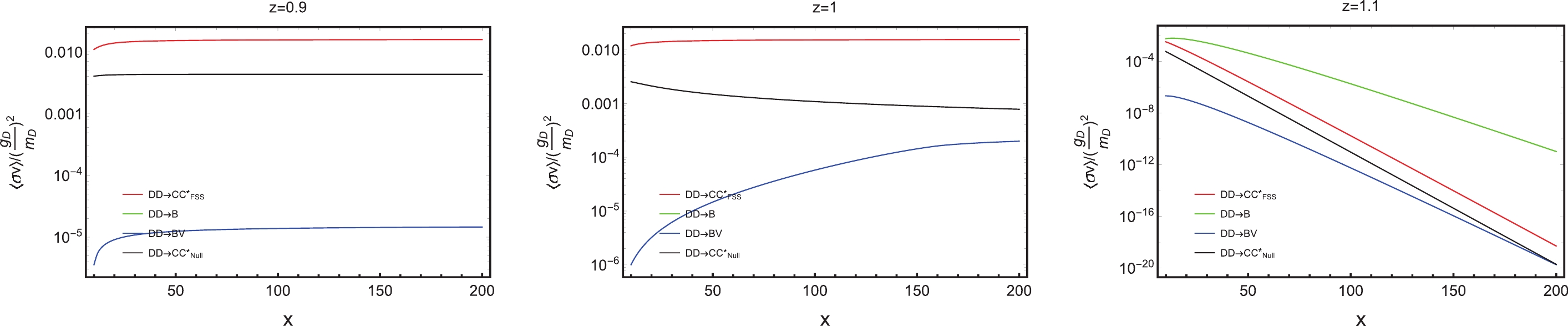
Figure 6. (color online) The thermal-averaged cross sections over a common factor,
$ g_D ^2 / m_D ^2 $ , at three parameters,$ z = 0.9, 1, 1.1 $ , and$ \alpha_{V}=0.5 $ . The red, green, blue, and black lines stand for$ \langle\sigma v\rangle_{\rm FSS} $ , the thermal-averaged FSS-corrected s-wave cross section;$ \langle\sigma v \rangle_{B} $ , the thermal-averaged s-wave FBS (without boson emission) formation cross section;$ \langle\sigma v \rangle_{BV} $ , the thermal-averaged p-wave FBS (with boson emission) formation cross section; and$ \langle\sigma v \rangle_{\rm w/o \ both} $ , the thermal-averaged cross section without any correction, respectively. The x is the ratio$ m_D/T $ . The y-axis is the thermal-averaged cross sections divided by a common factor.Furthermore, in Fig. 6, there is some difference between the left/middle panel from the right panel. The right panel represents the forbidden case. As x increases, the thermal-averaged cross sections become smaller. Because, as the temperature decreases, the initial particles become less energetic and the proportion of particles reaching the reaction threshold reduces. Meanwhile, in the left and middle panel, cross sections do not change much with temperature. Model I is a typical four point interaction, and the scattering matrix element does not relate with the initial particle's momentum.
The bound state can also be virtual as a propagator in the
$ DD \to B^* \to V V $ process. The corresponding corss section can be calculated by the Breit–Wigner formula [42, 43]. However, we do not need to consider the virtual bound state process here. Because for$ z>1 $ , the bound state generated by the process of$ DD \to B $ will decay and cause double counting; for$ z<1 $ , in the Breit–Wigner formula, the virtual bound process is suppressed by the factor,${\Big(m_B^{2} \Gamma^{2}\Big)}/{\Big(\left(s-m_B^{2}\right)^{2}+m_B^{2} \Gamma^{2}\Big)}$ , where$ \Gamma \sim \alpha_{V}^5 m_B $ and$ m_B \approx 2 m_C $ (assuming the dominate decay channel is$ B \to VV $ ). At the typical DM freeze-out temperature,$ x=25 $ ,$ (s-m_B^2) \sim ({12}/{25}) m_C^2 $ at$ z=1 $ . This factor is far away from its resonance pole. -
We already obtained the thermal-averaged cross sections, numerically, in Sec. III.B.1. Solving the Boltzmann equation is simple, as outlined in Sec. II.C. Similarly, we choose three parameters,
$ \alpha_{V} = 0.02,\; 0.1,\; 0.5 $ , and show the$ yield $ of DM as a function of x, considering different effects. In order to show the FBS formation effect, we choose other the parameters as$ z=1.1 $ (the forbidden case),$ m_D=1\;{\rm TeV} $ , and$ g_D=1 $ . As Fig. 7 shows, the purple line neglects both the FSS and FBS effects, the brown line neglects the FBS effect, and the green line incorporates the effects of FBS and FSS. In both Model I and Model II numerical calculations, we choose the other parameters in the Boltzmann equation as$ {{\rm d}g_{*s}}/{{\rm d}T}\simeq 0 $ ,$ g_*=g_{*s}=108.75 $ . We take$ 108.75 $ to account for the SM plus the two dark-photon degrees of freedom.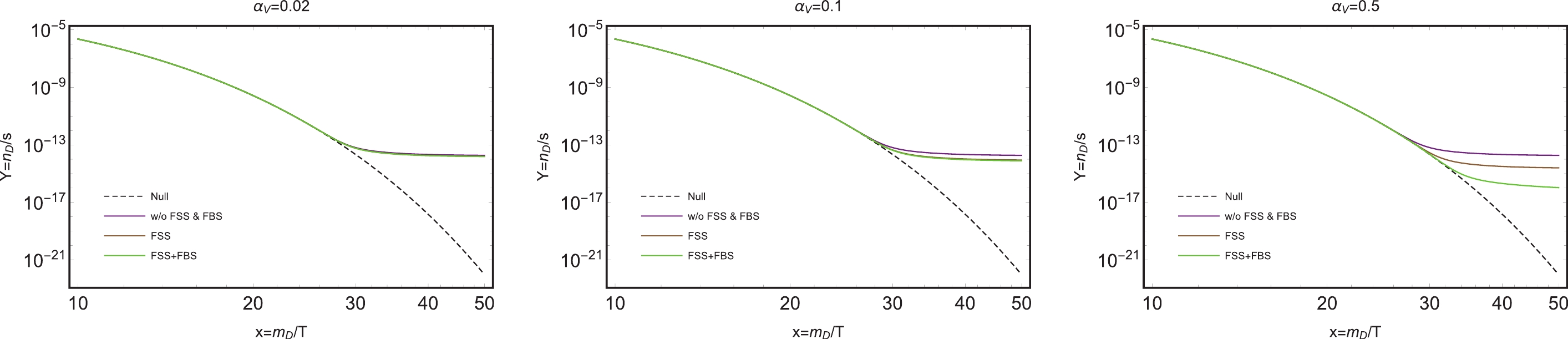
Figure 7. (color online) The evolution of the DM
$ yield $ as a function of$ x=m_D/T $ for the representative case$ m_D=1 \;{\rm TeV} $ ,$ z=1.1 $ , and$ g_D=1 $ and$ \alpha_{V}=0.02, \;0.1, \;0.5 $ . The purple line neglects both the FSS and FBS effects. The brown line neglects the FBS effect. The green line incorporates the effect of FBS and FSS. The black dashed line exhibits the naive thermal equilibrium abundance.Figure 7 shows the DM
$ yield $ considering different effects with the coupling constant,$ \alpha_{V} = 0.02, \;0.1, \;0.5 $ , respectively. In the left panel, for the electroweak-like scale interaction,$ \alpha_{V}=0.02 $ and both FSS and FBS effects hardly change the DM$ yield $ . As$ \alpha_{V} $ increases to$ 0.1 $ , the FSS effect starts to show some influence, but the FBS effect is still feeble as compared with the FSS effect. In the right panel,$ \alpha_{V} $ increases to$ 0.5 $ . The FBS shows a significant enhancement on the final$ yield $ of DM. It further reduces the relic abundance by 93% on top of the FSS effect. We note that for the forbidden case ($ z=1.1 $ ), all$ \langle\sigma v \rangle $ s quickly decrease with the decrease of temperature, as shown in the right panel of Fig. 6. Thus, the DM$ yield $ quickly reaches its asymptotic value after freeze-out. We have checked that the$ yield $ is nearly the same at$ x=50 $ and$ x=300 $ .Figures 5 and 7 show that the FBS formation effect and FSS effect are important in the DM relic abundance calculation when DM annihilation products are non-relativistic and have a large coupling with a light vector boson. In particular, when
$ \alpha_{V} $ is very large, the cross section of FBS formation without emission dominates for the forbidden region. -
Model I is a typical four-point interaction between DM and the annihilation products. Due to angular momentum conservation, in Model I, we only consider s-wave FSS effect, s-wave FBS formation without vector boson emission, and p-wave FBS formation with a vector boson emission. Next, we employ another model, which at the leading order gives the p-wave FSS effect, p-wave FBS formation without vector boson emission, and s-wave FBS formation with a vector boson emission.
In this model, DM consists of a complex scalar, S, which has scalar QED-like coupling with a heavy neutral vector boson, which we denote as
$ Z^\prime $ (but note that it is not the Z boson in Standard Model). Another complex scalar, C, couples with$ Z^\prime $ and another light-vector boson, V. The dark sector we explore in this model is summarized by the Lagrangian:$ \begin{array}{*{20}{l}} \mathcal{L}_{II}\supset|D_\mu C|^2+|D_\mu S|^2, \end{array} $

(31) where the covariant derivatives are
$ D^\mu C=\partial^\mu C+{\rm i}g_3V^\mu C+ {\rm i}g_5Z ^{\prime \mu} C $ and$D^\mu S=\partial^\mu S+{\rm i} g_6Z^{\prime \mu} S$ .At
$ zero $ temperature, the V mass is zero. In the thermal bath, same as in Model I, it has Debye mass$ m_V \sim g_VT $ . -
In this model, Fig. 8 shows the direct annihilation of DM without/with the FSS effect.
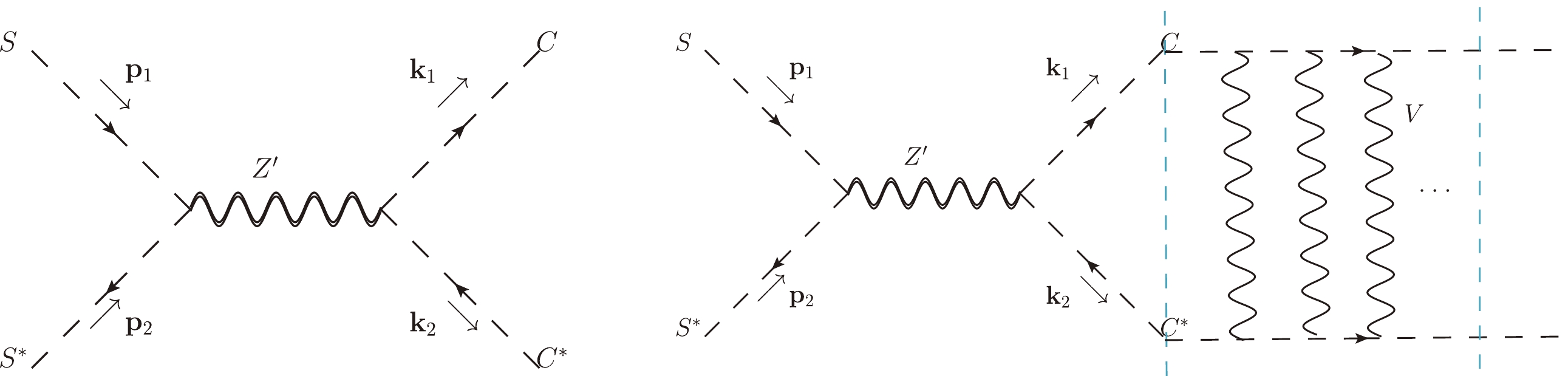
Figure 8. (color online) The Feynman diagrams for the
$ SS^\ast \rightarrow CC^\ast $ without/with the FSS effect.The scattering amplitude for the process
$ SS^*\rightarrow CC^* $ in the COM frame is$ {\rm i}\mathcal{M}_{SS^*\rightarrow CC^*} = -4{\rm i} g_5 g_6 \frac{|{\boldsymbol{p}}_1||{\boldsymbol{k}}_1|\cos\theta }{s-m_{Z^\prime}^2}, $

(32) where
$ {\boldsymbol{p}}_1,\;{\boldsymbol{k}}_1 $ are the 3-momentum$ s=(p_1+p_2)^2 $ . Because the matrix element is proportional to the final 3-momentum$ {\boldsymbol{k}}_1 $ , there is only the p-wave Sommerfeld effect.The cross section times relative velocity, v, of the incoming DM particles in the COM frame for this process is
$ \begin{aligned}[b] & (\sigma _{ann}v) =\frac{g_5 ^2 g_6 ^2}{24 \pi s} \frac{(s-4m_S^2)(s-4m_C ^2)}{(s-m_{Z^\prime}^2)^2} v_2, \\ & v_2=\sqrt{1-4m_C^2/s}. \end{aligned} $

(33) Again, the value under the square root must be larger than
$ zero $ for the "forbidden" case.Same as the Model I, the FSS effect can occur since the final state particles exchange vector boson, V. We still use the Coulomb-like potential to calculate the FSS and FBS effect. Considering the FSS effect for p-wave, the corrected cross section is
$ \begin{array}{*{20}{l}} (\sigma v)_{\rm FSS}= (\sigma _{ann}v) \ S_f , \end{array} $

(34) where
$ S_{ f}=\left(1+\left(\frac{\alpha_{V}}{2v_2}\right)^2\right)\frac{\pi\alpha_{V}/v_2}{1-{\rm e}^{-\pi\alpha_{V}/v_2}} $

(35) is the FSS factor,
$ S_ f $ is for the p-wave [44, 45], and$ \alpha_{V} = {g_3^2}/ {(4\pi)} $ . -
We get the scattering amplitude in Eq. (32) of
$ SS^*\rightarrow CC^\ast $ . As the last section outlined, the matrix element shows that the annihilation products should be in p-wave. We have already discussed the p-wave FBS formation in Model I, and we use the same techniques to calculate the cross section for$ SS^*\rightarrow B $ in Model II, as shown in Fig. 9.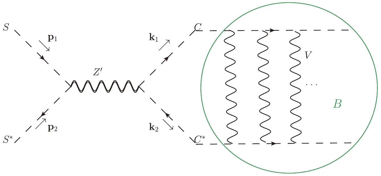
Figure 9. (color online) The Feynman diagrams for the
$ SS^\ast \rightarrow B $ annihilation.Using the
$ L=1 $ wave function in Eq. (23) and working in the COM frame, we obtain$ |\mathcal{M}_{SS^*\rightarrow B}|^2=\frac{\alpha_{V} ^5 g_5^2g_6^2 }{24\pi}\frac{m_C^4 (s-4m_S^2)}{(s-m_{Z^\prime}^2)^2} \left(\frac{1}{n^3}-\frac{1}{n^5}\right). $

(36) Then, we get the cross section times relative velocity according to [38]
$ (\sigma v)_B = \frac{2\pi}{s} |\mathcal{M}_{SS^*\rightarrow B}|^2 \ \delta \left(E_{\rm cm}^2 - m_B^2\right), $

(37) where
$ m_B $ is bound state mass, and the δ function ensures energy-momentum conservation. -
The FBS formation process,
$ SS^*\rightarrow BV $ , can be described by three Feynman diagrams shown in Fig. 10. The excessive energy can be carried away by a vector boson, V, emission.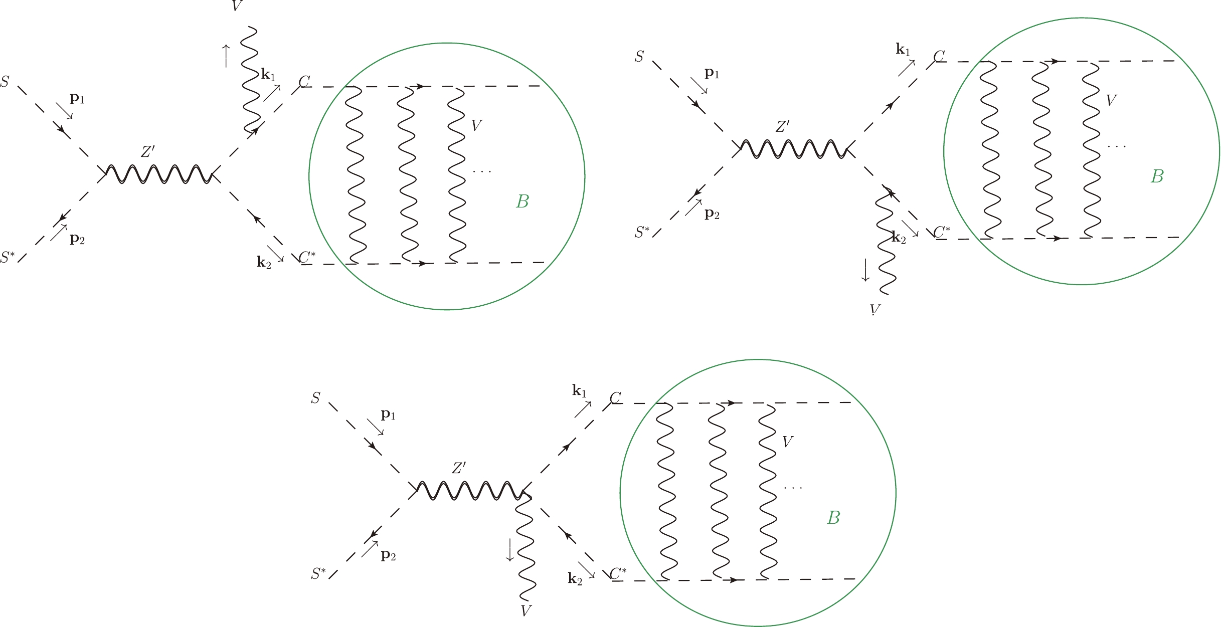
Figure 10. (color online) The Feynman diagrams for the
$ (CC^*) $ bound state production process,$ SS^*\rightarrow BV $ .The scattering amplitude for this process can be written as
$ \begin{aligned}[b] {\rm i}\mathcal{M}_{SS^*\rightarrow CC^*V} =&(-{\rm i}g_6)(p_1-p_2)^\mu\frac{-{\rm i}}{(p_1+p_2)^2-m_{Z^\prime}^2}\left[g_{\mu\nu}-\frac{(p_1+p_2)_\mu(k_1+k_2+q)_\nu}{m_{Z^\prime}^2}\right]\\ &\times(-{\rm i}g_5)(k_1+q-k_2)^\nu\frac{{\rm i}}{(k_1+q)^2-m_C^2}(-{\rm i}g_3)(k_1+k_1+q)^\beta \cdot\epsilon _\beta^*\\ &+(-{\rm i}g_6)(p_1-p_2)^\mu\frac{-{\rm i}}{(p_1+p_2)^2-m_{Z^\prime}^2}\left[g_{\mu\nu}-\frac{(p_1+p_2)_\mu(k_1+k_2+q)_\nu}{m_{Z^\prime}^2}\right]\\ &\times(-{\rm i}g_5)(k_1-(k_2+q))^\nu\frac{{\rm i}}{(k_2+q)^2-m_C^2}(-{\rm i}g_3)(-k_2-(k_2+q))^\beta\cdot\epsilon _\beta^*\\ &+(-{\rm i}g_6)(p_1-p_2)^\mu\frac{-{\rm i}}{(p_1+p_2)^2-m_{Z^\prime}^2}\left[g_{\mu\nu}-\frac{(p_1+p_2)_\mu(k_1+k_2+q)_\nu}{m_{Z^\prime}^2}\right]\times 2{\rm i}g_3g_5g^{\nu\beta}\cdot\epsilon _\beta^*\,. \end{aligned} $ 
(38) Because the final state emits a spin one vector boson, considering the angular momentum conservation, the FBS should be s-wave. Turning to the rest frame of the (
$ CC^* $ ) bound state, we rewrite Eq. (38) under the non-relativistic approximation and expand to the$ zeroth $ order of the final state relative momentum$ {\boldsymbol{k}} $ , as$ \mathcal{M}^j_{SS^*\rightarrow CC^*V} = \frac{-2g_3g_5g_6}{s-m_{Z^\prime}^2} \left[ (p_1 - p_2)^j- \frac{q^j}{2m_C\omega + m_V^2}((p_1 - p_2) \cdot q) \right], $

(39) where the index, j, stands for spatial 3-component.
The FBS effect can be calculated as in Model I; the matrix element is multiplied by the Fourier transform mode of the wave function (
$ L=0 $ ), which comprises the$ CC^* $ pair relative momentum,$ {\boldsymbol{k}} $ , and integrates out the relative momentum,$ {\boldsymbol{k}} $ . We get the scattering amplitude for the process$ SS^*\rightarrow BV $ $ \begin{aligned}[b] \mathcal{M}^j_{BV} = \sqrt{\frac{1}{m_C}}\int \frac{{\rm d}^3{\boldsymbol{k}}}{(2\pi)^3}\widetilde{\psi}^*({\boldsymbol{k}}) \ \mathcal{M}^j_{SS^*\rightarrow CC^*V} \end{aligned} $

$ \begin{aligned}[b] \quad = \sqrt{\frac{1}{m_C}}\psi^*(0) \ \mathcal{M}^j_{SS^*\rightarrow CC^*V}. \end{aligned} $

(40) Similarly, the s-wave bound state formation scattering amplitude is proportional to the value of the wave function at
$ {\boldsymbol{r}}=0 $ . The hydrogen-like wave function used here is the$ L=0 $ part, same as Eq. (15).Sum over the polarization of the vector boson, V, then we obtain
$ \begin{aligned}[b] \sum_{\epsilon}|\mathcal{M}_{SS^*\rightarrow BV}|^2 =&\Bigg(\frac{-2g_3g_5g_6}{s-m_{Z^\prime}^2}\Bigg)^2\frac{1}{m_C}\frac{1}{\pi(na_0)^3}\Bigg[(s-4m_S ^2)\\&-\frac{(2|{\boldsymbol{p}}||{\boldsymbol{q}}|\cos\theta)^2}{|{\boldsymbol{q}}|^2+m_V^2}\\ &+\frac{(-2|{\boldsymbol{p}}||{\boldsymbol{q}}|\cos\theta)^2|{\boldsymbol{q}}|^2}{(2m_C\omega+m_V^2)^2}\left(1-\frac{|{\boldsymbol{q}}|^2}{|{\boldsymbol{q}}|^2+m_V^2}\right)\\ &+\frac{8(|{\boldsymbol{p}}||{\boldsymbol{q}}|\cos\theta)^2}{2m_C\omega+m_V^2}\left(1-\frac{|{\boldsymbol{q}}|^2}{|{\boldsymbol{q}}|^2+m_V^2}\right)\Bigg]. \end{aligned} $

(41) The cross section times relative velocity, v, of the incoming DM particles for the process
$ SS^*\rightarrow B(L=0)V $ is$ \begin{array}{*{20}{l}} (\sigma v)_{SS^*\rightarrow BV}=C\left[\left(3-B\right)+2A\left(1-B\right)+A^2\left(1-B\right)\right], \end{array} $

(42) where
$ \begin{aligned}[b] A=&\frac{|{\boldsymbol{q}}|_{\rm cm}^2}{2m_C\omega+m_V^2},\quad B=\frac{|{\boldsymbol{q}}|_{\rm cm}^2}{|{\boldsymbol{q}}|_{\rm cm}^2+m_V^2},\\ C=&\frac{\alpha_{V}^4 g_5^2g_6^2}{6\pi n^3} \frac{m_C^2 (s-4m_S ^2)}{s(s-m_{Z^\prime}^2)^2}\frac{|{\boldsymbol{q}}|_{\rm cm}}{\sqrt{s}}. \end{aligned} $

(43) In the low temperature limit,
$ m_V \sim g T = 0 $ , only the first term in the square brackets is left in Eq. (42)$ (\sigma v)_{SS^*\rightarrow BV}= \frac{\alpha_{V}^4 g_5^2g_6^2}{3\pi n^3} \frac{m_C^2 (s-4m_S ^2)}{s(s-m_{Z^\prime}^2)^2}\frac{|{\boldsymbol{q}}|_{\rm cm}}{\sqrt{s}}. $

(44) This term comes from the third diagram in Fig. 10, so in Model II, there is no infrared divergence for the
$ SS^*\rightarrow BV $ process. The emitted vector boson energy in the rest frame of the bound state is$ \begin{array}{*{20}{l}} \begin{aligned} & \omega =\frac{s-m_B^2-m_V^2}{2m_B}.\\ \end{aligned} \end{array} $

(45) The formula about
$ |{\boldsymbol{q}}|_{\rm cm} $ is same as what we give in Eq. (30). It is obvious that the vector boson momentum,$ |{\boldsymbol{q}}|_{\rm cm} $ , must be larger than$ zero $ . It decides the minimum$ s_{\rm min} $ . -
As in Sec. III.B, we plot the thermal-averaged cross sections as a function of the mass ratio of the final and initial state particles at three parameters,
$ \alpha_{V} = 0.02, \;0.1, 0.5 $ . We normalize the other particles' mass by the DM mass,$ z\equiv m_C/m_S $ ; then, we plot the thermal-averaged cross section evolution as a function of x at three parameters$ z = 0.9, \;1,\; 1.1 $ and$ \alpha_{V} = 0.5 $ . -
The cross sections and kinematic threshold,
$ s_{\rm min} $ , for three processes are summarized in Table 2. In the numerical calculation, we only consider$ n=2 $ for the$ SS^*\rightarrow B $ and$ n=1 $ for the$ SS^*\rightarrow BV $ .channel $ (\sigma v) $ 

$s_{\rm min}$ 

$ SS^*\rightarrow CC^* $ 

$\dfrac{g_5 ^2 g_6 ^2}{24 \pi s} \dfrac{(s-4m_S^2)(s-4m_C ^2)}{(s-m_{Z^\prime}^2)^2} v_2\left(1+\left(\dfrac{\alpha_{V} }{2v_2}\right)^2\right)\dfrac{\pi\alpha_{V}/v_2}{1-{\rm e}^{-\pi\alpha_{V}/v_2} }$ 

${\rm Max}[4 m_S^2,4m_C^2]$ 

$ SS^*\rightarrow B $ 

$\dfrac{\alpha_{V} ^5 g_5^2g_6^2 }{12s}\dfrac{m_C^4 (s-4m_S^2)}{(s-m_{Z^\prime}^2)^2} \left(\dfrac{1}{n^3}-\dfrac{1}{n^5}\right)\delta \left(E_{\rm cm}^2 - m_B^2\right)$ 

$ 4 m_S^2 $ 

$ SS^*\rightarrow BV $ 

$ C\left[\left(3-B\right)+2A\left(1-B\right)+A^2\left(1-B\right)\right] $ 

${\rm Max}[4 m_S^2, \ (m_B+m_V)^2]$ 

Table 2. Cross sections and kinematical forbidden limits for Model II.
From the above table, it is obvious that a strong enhancement occurs when the mass of the propagator
$ m_{Z^\prime} \approx 2 m_S $ ; in fact, it is the resonance enhancement [34, 42, 43]. In this study, we do not discuss the details about the resonance enhancement and just focus on the parameter region where$ m_{Z^\prime} \gg m_S $ and using approximation$ 1/(s-m_{Z^\prime}^2)^2 \to 1/m_{Z^\prime}^4 $ for the square of$ Z^\prime $ propagator to avoid this effect.We can calculate the thermal-averaged cross sections from Table 2, following Eq. (3) in Sec. II.B. Fig. 11 shows the thermal-averaged cross sections as a function of the mass ratio of the final and initial state particles at a typical freeze-out value,
$ x=25 $ . The red, green, blue, and black lines stand for$ \langle\sigma v\rangle_{\rm FSS} $ ,$ \langle\sigma v \rangle_{B} $ ,$ \langle\sigma v \rangle_{BV} $ , and$ \langle\sigma v \rangle_{\rm w/o \ both} $ over a common factor$ g_5 ^2 g_6 ^2 m_S ^2/m_{Z^\prime}^4 $ , respectively.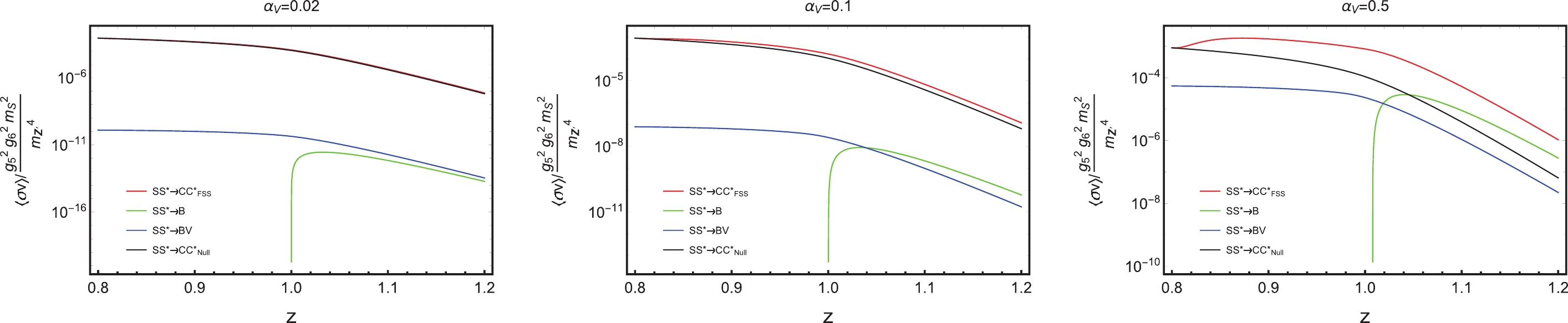
Figure 11. (color online) The thermal-averaged cross sections over a common factor,
$ g_5 ^2 g_6 ^2 m_S ^2/m_{Z^\prime}^4 $ at three parameters$\alpha_{V} = 0.02,\; 0.1,\; 0.5$ , at a typical freeze-out value,$ x=m_S/T=25 $ . The red, green, blue, and black lines stand for$ \langle\sigma v\rangle_{\rm FSS} $ , the thermal-averaged FSS-corrected p-wave cross section;$ \langle\sigma v \rangle_{B} $ , the thermal-averaged FBS (without boson emission) p-wave cross section;$ \langle\sigma v \rangle_{BV} $ , the thermal-averaged FBS (with boson emission) s-wave cross section; and$ \langle\sigma v \rangle_{\rm w/o both} $ , the thermal-averaged cross section without any FSS and FBS, respectively. z is the mass ratio$ m_C/m_S $ . The y-axis is the thermal-averaged cross sections divided by a common factor.It can be seen from Fig. 11that
$ \langle\sigma v \rangle_{BV} $ is comparable to$ \langle\sigma v \rangle_{B} $ , while in Model I, the former is much smaller than the latter (Fig. 5). The reason is in Model II, it is the s-wave FBS formation with vector boson emission, while in Model I, it is p-wave FBS formation with vector boson emission. In Model II, FBS formation without emission is p-wave. Its contribution is suppressed comparing to that in Model I in which FBS formation without emission is s-wave. On the other hand, at$ \alpha_{V}=0.5 $ , while in Model I,$ \langle\sigma v \rangle_{B} $ is larger than$ \langle\sigma v \rangle_{\rm FSS} $ . The former is still smaller than the latter, though they are getting closer.Figure 12 shows the evolution of thermal-averaged cross sections of Model II as temperature drops. In the left and the middle panels, the
$ \langle\sigma v \rangle_{B} $ does not appear for the same reason as Model I. The right panel is for the forbidden case. It is the same as Model I, at low temperature, fewer initial particles can reach the threshold. Therefore, the thermal-averaged cross sections become smaller as temperature decreases. However, in the left and the middle panel, the trend of the lines are different in Fig. 6 and Fig. 12. It is because in Model II, the three point vertices are proportional to the momentum. That is why the thermal-averaged cross sections are smaller with decreasing temperature.
Figure 12. (color online) The thermal-averaged cross sections over a common factor,
$ g_5 ^2 g_6 ^2 m_S ^2/m_{Z^\prime}^4 $ at three parameters$ z = 0.9, 1, 1.1 $ and$ \alpha_{V}=0.5 $ . The red, green, blue, and black lines stand for$ \langle\sigma v\rangle_{\rm FSS} $ , the thermal-averaged FSS-corrected p-wave cross section;$ \langle\sigma v \rangle_{B} $ , the thermal-averaged FBS (without boson emission) p-wave cross section;$ \langle\sigma v \rangle_{BV} $ , the thermal-averaged FBS (with boson emission) s-wave cross section; and$ \langle\sigma v \rangle_{\rm w/o both} $ , the thermal-averaged cross section without any FSS and FBS, respectively. z is the mass ratio$ m_C/m_S $ . The y-axis is the thermal-averaged cross sections divided by a common factor.The right panel of Fig. 12 indicates that the
$ SS^*\rightarrow BV $ process may provide a significant, indirect detection signal for forbidden dark matter. Because the process$ SS^\ast \to BV $ becomes more and more important as x decreases, it dominates in low temperatures ($ x>150 $ ). -
We have already obtained the thermal-averaged cross sections numerically in Sec. IV.B.1. Solving the Boltzmann equation is simple, as outlined in Sec. II.C, by substituting
$ m_D $ with$ m_S $ . Again, we choose three parameters,$ \alpha_{V} = 0.02,\; 0.1,\; 0.5 $ , and show the$ yield $ of DM as a function of x considering different effects. Other parameters are chosen as$ z=1.1 $ (the forbidden case),$ m_S=500\;{\rm GeV} $ , and$ g_5 ^2 g_6 ^2 m_S ^2/m_{Z^\prime}^4= 10^{-6} \rm GeV^{-2} $ . As Fig. 13 shows, the purple line neglects both FSS and FBS effects, the brown line neglects FBS effect, and the green line incorporates the effects of FBS and FSS.
Figure 13. (color online) The evolution of the DM
$ yield $ as a function of$ x=m_S/T $ for the representative case$ m_S=500 \;{\rm GeV }$ ,$ z=1.1 $ ,$ g_5 ^2 g_6 ^2 m_S ^2/m_{Z^\prime}^4= 10^{-6} \;{\rm GeV}^{-2} $ , and$ \alpha_{V}=0.02,\;0.1,\;0.5 $ . The purple line neglects both FSS and FBS effects. The brown line neglects FBS effect. The green line incorporates the effects of FBS and FSS. The black dashed line exhibits the naive thermal equilibrium abundance.Compared to Model I, the FBS effect is milder; the p-wave FSS effect also has a significant enhancement on DM annihilation. In Model II, the FBS effect without emission is p-wave. Although the FBS effect with emission is s-wave, it is still suppressed by order
$ \alpha_{V} $ because of a vector boson emission. However, in the right panel,$ \alpha_{V}=0.5 $ , and the FBS effect contribution is still visible. It further reduces the relic abundance by 13% on top of the FSS effect.Figures 11 and 13 show that the FBS formation effect and FSS effects are important in DM relic abundance calculation when DM annihilation products are non-relativistic and have a large coupling with a light vector boson.
-
We investigate the FBS effect on DM relic abundance in this study. We employ two DM models and calculate the FSS effect and FBS effect using Coulomb-like potential approximation. We give the numerical results considering those effects, which demonstrate that the FBS has a significant effect on the DM relic abundance if DM annihilation products move non-relativistically and there is some long-range force between them, particularly in the forbidden dark matter cases.
Compared to previous works on this subject, the FBS effect, which had not been previously taken into account, expands the scope of both the DM abundance calculation and the complementary ways of experimental detection. We point out the following salient features of this work:
(a) Most of the previous work focuses on the initial state bound state (IBS) effect. We stress that the same argument could be extended to the FBS effect. We provide two models to show that the FBS effect has a significant influence on the DM relic abundance compared to the FSS effect, especially for the "forbidden" cases.
(b) We find the usual sub-leading FBS formation process cannot be negligible compared to the lead process and has the potential to give the indirect detection signals.
(c) We also consider that the p-wave FSS effect in this work compares to the one in [21].
-
F. L. thanks Xiaoyi Cui and Shu Lin for helpful discussions.
Final bound-state formation effect on dark matter annihilation
- Received Date: 2022-04-03
- Available Online: 2022-09-15
Abstract: If two annihilation products of dark matter (DM) particles are non-relativistic and couple to a light force mediator, their plane wave functions are modified due to multiple exchanges of the force mediator. This gives rise to the final state Sommerfeld (FSS) effect. It is also possible that the final state particles form a bound state. Both the FSS effect and final bound-state (FBS) effect need to be considered in the calculation of the DM relic abundance. The annihilation products can be non-relativistic if their masses are comparable to those of the annihilating DM particles. We study the FSS and FBS effects in the mass-degenerate region using two specific models. Both models serve to illustrate different partial-wave contributions in the calculations of the FSS and FBS effects. We find that the FBS effect can be comparable to the FSS effect when the annihilation products couple strongly with a light force mediator. Those effects significantly modify the DM relic abundance.


 DownLoad: