


 Abstract
 HTML
HTML Reference
 Related
 PDF
PDF


-
In general relativity, the study of geodesic motion of a test particle in curved space-time is the best probe for understanding the physics and geometry of gravitational objects. It leads to the possibility of solving the problem of Mercury perihelion, which is considered one of the triumphs of the general theory of relativity. The classification of stable and unstable orbits is performed by drawing effective potentials and checking their behavior at different points.
There are many references in the literature that are concerned with detailed studies of the geodesic movement of black holes, see for instance Refs. [1–25]. In this paper, we are interested in studying the geodesic motion in non-commutative space-time by imposing further commutation relations between the position coordinates, themselves. This non-commutativity leads to the modification of the Heisenberg uncertainty relations in such a way that prevents measuring positions to a better accuracy than the Planck length. Non-commutativity is mainly motivated by string theory because of its limit in the presence of a background field [26–33]. This idea results in the concept of quantum gravity since quantifying space-time leads to quantifying gravity. Quantum gravity effects can be neglected in the low-energy limit, while in the strong gravitational field of a black hole, these effects have to be considered.
In non-commutative space-time the coordinate and momentum operators satisfy the following commutation relations
$ \begin{equation} [x^{\mu},x^{\nu}]={\rm i}\,\Theta^{\mu\nu}\,, \end{equation} $

(1) where
$ \Theta^{\mu\nu} $ is an anti-symmetric real matrix, which determines the fundamental cell discretization of space-time much in the same way as the Planck constant,$ \hbar $ , which discretizes the phase space. Moreover,$ x^{\mu} $ are the coordinate operators in a non-commutative space-time defined by the following transformations:$ \begin{equation} \hat{x}^{\mu}=x^{\mu}-\Theta^{\mu\nu}\,p_{\nu}\,. \end{equation} $

(2) In the non-commutative theory, ordinary products are changed to star (Moyal) products "
$ * $ ," which for two arbitrary functions,$ f(x) $ and$ g(x) $ , is defined by$ \begin{equation} (f*g)(x)=f(x)\exp\left[\frac{\rm i}{2}\,\Theta^{\mu\nu}\overleftarrow{\partial}_{\mu}\overrightarrow{\partial}_{\nu}\right]g(x)\,. \end{equation} $

(3) There has recently been a lot of interest in studies that investigate modifications introduced by non-commutativity on the geodesic structure in a black hole [34–45]. The treatment of gravity in the context of the non-commutative geometry approach can be studied by two theories. In the first approach one adapts general relativity to the noncommutative setting in an intuitive way [46, 47]. While the second theory, it is based on axiomatically developing noncommutative versions of the Riemannian geometry [46–50]. This study applies the first theory that describes noncommutative gravity as noncommutative gauge theory. Here, we use a gravity gauge theory in non-commutative space-time with star products and Seiberg-Witten maps [51]. Non-commutative gauge gravity is a theory of general relativity in curved space-time with preservation of non-commutative space-time and is partly based on implementing symmetries on flat non-commutative space-time. In gauge theory of gravity, the action transforms under ordinary Lorentz transformations of the ordinary fields since these ordinary transformations, via the Seiberg-Witten map, induce the non-commutative canonical transformations of non-commutative fields under which the noncommutative action is invariant [52–54].
Our work, in this context, aims to write the geodesic equation that arises from the metric tensor, which has been corrected using star products between tetrad fields and Seiberg-Witten maps. We, additionally, obtain non-commutative corrections for each of the effective potentials and the deviation angle per revolution and discuss the issue of the stability of circular orbits in a non-commutative Schwarzschild geometry.
This paper is organized as follows. In Sec. II, we present the non-commutative corrections to the metric field using star products between tetrad fields and Seiberg-Witten maps. In Sec. III, we calculate the non-commutative geodesic equation and obtain the non-commutative effective potentials up to second order in the non-commutativity parameter, and we determine the condition for the stability of the circular orbits of particles in noncommutative Schwarzschild space-time. We then calculate the non-commutative adjustment to the perihelion rotation value and give an estimate for the non-commutative parameter. In the last section, we present our concluding remarks.
-
Using the tetrad and spin connection formalism in the gauge theory of gravity is unavoidable because of the requirement to describe the spinor fields in this theory. We denote the tetrad fields by
$ e^{a}_{\mu} $ , with$ a=0,1,2,3 $ , and the spin connection by$ \omega^{ab}_{\mu}(x)=-\omega^{ba}_{\mu}(x) $ , with$ [ab]=[01], [02],[03],[12],[13],[23] $ . Then the Ricci scalar is given by$ \begin{equation} R=e_{a}^{\mu}\,e_{b}^{\nu}\,R^{ab}_{\mu\nu}\,, \end{equation} $

(4) where
$ e_{a}^{\mu} $ denotes the inverse of$ e^{a}_{\mu} $ satisfying the usual properties$ \begin{equation} e^{a}_{\mu}\,e_{b}^{\mu}=\delta^{a}_{b}\,,\qquad e^{a}_{\mu}\,e_{a}^{\nu}=\delta^{\nu}_{\mu}\,, \end{equation} $

(5) and
$ R^{ab}_{\mu\nu} $ denotes the curvature tensor$ \begin{equation} R^{ab}_{\mu\nu}=\partial_{\mu}\omega^{ab}_{\nu}-\partial_{\nu}\omega^{ab}_{\mu}+\left(\omega^{ac}_{\mu}\,\omega^{db}_{\nu}-\omega^{ac}_{\nu}\,\omega^{db}_{\mu}\right)\eta_{cd}\,. \end{equation} $

(6) The action of the pure gravity in the gauge theory reads
$ \begin{equation} S_{g}=\frac{1}{16\pi G}\int {\rm d}^{4}xe R=\frac{1}{16\pi G}\int {\rm d}^{4}xe e_{a}^{\mu}e_{b}^{\nu}R^{ab}_{\mu\nu}\,, \end{equation} $

(7) where
$ e={\rm det}(e^{a}_{\mu}) $ . Using the variational principle,$ \delta S=0 $ , for the action in (7) with respect to$ e^{a}_{\mu} $ , we obtain the field equation for the gravitational potentials ,$ e^a_\mu $ , in vacuum$ \begin{equation} R^a_{\mu}=0\,, \end{equation} $

(8) with
$ R^a_{\mu}=R^{ab}_{\mu\nu}e^{\nu}_b $ being the Ricci tensor.We consider the general solution for the equation of the gravitational field (8) in the case of static and spherical symmetry with the metric
$ \begin{equation} {\rm d}s^{2}=-A^{2}(r){\rm d}t^{2}+B^{2}(r){\rm d}r^{2}+r^{2}({\rm d}\theta^{2}+{\rm sin}^{2}\theta {\rm d}\phi^{2})\,, \end{equation} $

(9) where
$ A(r) $ and$ B(r) $ are functions which depend only on the radius, r. The tetrad formulation of general relativity allows us to write the tetrad components as$ \begin{equation} g_{\mu\nu}=e^{a}_{\mu}e_{a\nu} \,. \end{equation} $

(10) We choose a particular form of non-diagonal tetrad fields satisfying the relation (10) as follows
$ \begin{equation} e^{a}_{\mu}=\left[\begin{array}{cccc} A(r) & 0 & 0 & 0 \\ 0 & B(r)\sin\theta \cos\phi & r \cos\theta \cos\phi & -r \sin\theta \sin\phi \\ 0 & B(r)\sin\theta \sin\phi & r \cos\theta \sin\phi & r \sin\theta \cos\phi \\ 0 & B(r)\cos\theta & -r \sin\theta & 0 \end{array} \right] \,. \end{equation} $

(11) We note that this particular form of tetrad fields can be used for a stationary observer at spatial infinity [40].
The non-zero components of the spin connection for this tetrad field are
$ \begin{aligned}[b] \omega^{01}_{\mu}=&\left(\frac{A'(r)}{B(r)}\sin\theta \cos\phi,0,0,0\right),\\\omega^{02}_{\mu}=&\left(\frac{A'(r)}{B(r)}\sin\theta \sin\phi,0,0,0\right), \end{aligned} $

(12) $ \begin{aligned}[b] \omega^{03}_{\mu}=&\left(\frac{A'(r)}{B(r)}\cos\theta ,0,0,0\right),\\\omega^{12}_{\mu}=&\left(0,0,0,\left[1-\frac{1}{B(r)}\right]\sin^{2}\theta\right),\end{aligned} $

(13) $ \begin{aligned}[b] \omega^{13}_{\mu}=&\Bigg(0,0,-\left[1-\frac{1}{B(r)}\right]\cos\phi,\\&\left[1-\frac{1}{B(r)}\right]\sin\theta \cos\theta \sin\phi\Bigg),\end{aligned} $

(14) $ \begin{aligned}[b] \omega^{23}_{\mu}=&\Bigg(0,0,-\left[1-\frac{1}{B(r)}\right]\sin\phi,\\&-\left[1-\frac{1}{B(r)}\right]\sin\theta \cos\theta \cos\phi\Bigg). \end{aligned} $

(15) Using Eq. (6), the spin connection, and the tetrads fields, we obtain the non-zero components of the curvature tensor,
$ R^{ab}_{\mu\nu} $ , which are needed in the derivation of the expressions for the deformed tetrad fields$ \begin{aligned}[b] R^{01}_{01}=&-\left[\frac{A''(r)}{B(r)}-\frac{A'(r)B'(r)}{B^{2}(r)}\right]\sin\theta \cos\phi,\\ R^{01}_{02}=&-\frac{A'(r)}{B^{2}(r)}\cos\theta \cos\phi, \end{aligned} $

(16) $ \begin{aligned}[b] R^{01}_{03}=&\frac{A'(r)}{B^{2}(r)}\sin\theta \sin\phi,\\ R^{02}_{01}=&-\left[\frac{A''(r)}{B(r)}-\frac{A'(r)B'(r)}{B^{2}(r)}\right]\sin\theta \sin\phi , \end{aligned} $

(17) $ \begin{aligned}[b] \quad \;\;\;\;\;\, R^{02}_{02}=&-\frac{A'(r)}{B^{2}(r)}\cos\theta \sin\phi,\\ R^{02}_{03}=&-\frac{A'(r)}{B^{2}(r)}\sin\theta \cos\phi,\\ R^{03}_{02}=&\frac{A'(r)}{B^{2}(r)}\sin\theta , \end{aligned} $

(18) $ \begin{aligned}[b] \;\;\;\;\;\;\;\;\;\;R^{03}_{01}=&-\left[\frac{A''(r)}{B(r)}-\frac{A'(r)B'(r)}{B^{2}(r)}\right]\cos\theta,\\ R^{12}_{23}=&\left[1-\frac{1}{B^{2}(r)}\right]\sin\theta \cos\theta, \end{aligned} $

(19) $ \begin{aligned}[b] \;\;\;\;\;\;\;\;\;\;R^{12}_{13}=&\frac{B'(r)}{B^{2}(r)}{\rm sin}^{2}\theta,\\ R^{13}_{12}=&-\frac{B'(r)}{B^{2}(r)}\cos\phi,\\ R^{13}_{13}=&\frac{B'(r)}{B^{2}(r)}\sin\theta \cos\theta \sin\phi, \end{aligned} $

(20) $ \begin{aligned}[b] R^{13}_{23}=&-\left[1-\frac{1}{B^{2}(r)}\right]\sin^{2}\theta \sin\phi,\\ R^{23}_{13}=&-\frac{B'(r)}{B^{2}(r)}\sin\theta \cos\theta \cos\phi, \end{aligned} $

(21) $ \begin{aligned}[b] R^{23}_{12}=&-\frac{B'(r)}{B^{2}(r)}\sin\phi,\\ R^{23}_{23}=&\left[1-\frac{1}{B^{2}(r)}\right]\sin^{2}\theta \cos\phi, \end{aligned} $

(22) where
$ A'(r) $ ,$ B'(r) $ and$ A''(r) $ denote the derivatives of first and second-order with respect to the r-coordinate.In non-commutative space-time, in order to find the deformed tetrad fields,
$ \hat{e}^{a}_{\mu}(x,\Theta) $ , we use the Seiberg-Witten map, which describes the tetrad fields as a power series in Θ up to the second order [55]$ \begin{aligned}[b] \hat{e}^{a}_{\mu}(x,\Theta)= &e^{a}_{\mu}(x)-{\rm i}\Theta^{\nu\rho}e^{a}_{\mu\nu\rho}(x) \\&+\Theta^{\nu\rho}\Theta^{\lambda\tau}e^{a}_{\mu\nu\rho\lambda\tau}(x)+{\cal{O}}(\Theta^{3}) \,, \end{aligned} $

(23) where
$ e^{a}_{\mu\nu\rho}=\frac{1}{4}[\omega^{ac}_{\nu}\partial_{\rho}e^{d}_{\mu}+(\partial_{\rho}\omega^{ac}_{\mu}+R^{ac}_{\rho\mu})e^{d}_{\nu}]\eta_{cd}\,, $

(24) $ \begin{aligned}[b] e^{a}_{\mu\nu\rho\lambda\tau}=&\frac{1}{32}\left[2\{R_{\tau\nu},R_{\mu\rho}\}^{ab}e^{c}_{\lambda}-\omega^{ab}_{\lambda}(D_{\rho}R_{\tau\nu}^{cd}+\partial_{\rho}R_{\tau\nu}^{cd})e^{m}_{\nu}\eta_{dm}\right.\\ &-\{\omega_{\nu},(D_{\rho}R_{\tau\nu}+\partial_{\rho}R_{\tau\nu})\}^{ab}e^{c}_{\lambda}-\partial_{\tau}\{\omega_{\nu},(\partial_{\rho}\omega_{\mu}\\&+R_{\rho\mu})\}^{ab}e^{c}_{\lambda}-\omega^{ab}_{\lambda}\left(\omega^{cd}_{\nu}\partial_{\rho}e^{m}_{\mu}+\left(\partial_{\rho}\omega_{\mu}^{cd}+R_{\rho\mu}^{cd}\right)e^{m}_{\nu}\right)\eta_{dm}\\&+2\partial_{\nu}\omega_{\lambda}^{ab}\partial_{\rho}\partial_{\tau}e^{c}_{\lambda} -2\partial_{\rho}\left(\partial_{\tau}\omega_{\mu}^{ab}+R_{\tau\mu}^{ab}\right)\partial_{\nu}e^{c}_{\lambda}\\&-\{\omega_{\nu},(\partial_{\rho}\omega_{\lambda}+R_{\rho\lambda})\}^{ab}\partial_{\tau}e^{c}_{\mu} -\left(\partial_{\tau}\omega_{\mu}+R_{\tau\mu}\right)\\&\times\left(\omega^{cd}_{\nu}\partial_{\rho}e^{m}_{\lambda}+\left((\partial_{\rho}\omega_{\lambda}+R_{\rho\lambda})\right)e^{m}_{\nu}\right)\eta_{dm}\Big]\eta_{cb} \,, \end{aligned} $

(25) and
$ \begin{aligned}[b] \{\alpha,\beta\}^{ab}=&\left(\alpha^{ac}\beta^{db}+\beta^{ac}\alpha^{db}\right)\eta_{cd}\,,\\ [\alpha,\beta]^{ab}=&\left(\alpha^{ac}\beta^{db}-\beta^{ac}\alpha^{db}\right)\eta_{cd}\,. \end{aligned} $

(26) $ D_{\mu}R_{\rho\sigma}^{ab}=\partial_{\mu}R^{ab}_{\rho\sigma}+\left(\omega_{\mu}^{ac}R^{db}_{\rho\sigma}+\omega_{\mu}^{bc}R^{da}_{\rho\sigma}\right). $

(27) The complex conjugate,
$ \hat{e}^{a\dagger}_{\mu}(x,\Theta) $ , of the deformed tetrad field is obtained from the Hermitian conjugate of the relation (23)$ \begin{aligned}[b] \hat{e}^{a\dagger}_{\mu}(x,\Theta)= &e^{a}_{\mu}(x)+{\rm i}\Theta^{\nu\rho}e^{a}_{\mu\nu\rho}(x) \\&+\Theta^{\nu\rho}\Theta^{\lambda\tau}e^{a}_{\mu\nu\rho\lambda\tau}(x)+{\cal{O}}(\Theta^{3}) \,,\end{aligned}$

(28) and the real deformed metric is given by [52]
$ \begin{equation} \tilde{g}_{\mu\nu}(x,\Theta)=\frac{1}{2}\left[\hat{e}^{a}_{\mu}*\hat{e}^{b\dagger}_{\nu}+\hat{e}^{a}_{\nu}*\hat{e}^{b\dagger}_{\mu}\right]\eta_{ab} \,. \end{equation} $

(29) Using the Seiberg-Witten map (25) we obtain the deformed tetrad field,
$ \hat{e}^{a}_{\mu}(x,\Theta) $ , and its Hermitian conjugate,$ \hat{e}^{a\dagger}_{\mu}(x,\Theta) $ , given by relations (23) and (28). To simplify the calculations, we only consider space-space non-commutativity,$ \Theta_{0i}=0 $ , due to the known problem with unitary; hence, we choose the following metric for the non-commutativity parameter,$ \Theta^{\mu\nu} $ $ \begin{equation} \Theta^{\mu\nu}=\left(\begin{matrix} 0 & 0 & 0 & 0 \\ 0 & 0 & 0 & \Theta \\ 0 & 0 & 0 & 0 \\ 0 & -\Theta & 0 & 0 \end{matrix} \right), \qquad \mu,\nu=0,1,2,3 \,, \end{equation} $

(30) where Θ is a real positive constant.
The non-zero components of the non-commutative tetrad fields,
$ \hat{e}^{a}_{\mu} $ , are$ \begin{aligned}[b] \hat{e}^{0}_{0}=&A(r)+\frac{\Theta^{2}}{32B^{4}(r)}\left\{-4B(r)(4rB'(r)A''(r)+A'(r)(2B'(r)+rB''(r)))\right.+16rA'(r)B'^{2}(r)+B^{3}(r)(A'(r)B'(r)\\&+4A''(r))+B^{2}(r)(-3A'(r)B'(r)\left.+4(A''(r)+rA'''(r)))\right\} \sin^{2}\theta+{\cal{O}}(\Theta^{3}), \end{aligned} $ 
(31) $ \begin{aligned}[b] \hat{e}^{1}_{1}=&B(r)\sin\theta \cos\phi+\frac{{\rm i}\Theta}{4}B'(r)\sin\theta \sin\phi+\frac{\Theta^{2}}{64B^{3}(r)}\left\{8(2B'(r)-B(r)B''(r))\sin^{2}\theta\right.+B^{3}(r)B''(r)(3+\cos2\theta)\\&+B(r)(B'^{2}(r)-B(r)B''(r))(1+3\cos2\theta)\Big\}\sin\theta \cos\phi+{\cal{O}}(\Theta^{3}) \end{aligned} $

(32) $ \begin{aligned}[b] \quad\quad \;\;\;\hat{e}^{2}_{1}=&B(r)\sin\theta \sin\phi-\frac{{\rm i}\Theta}{4}B'(r)\sin\theta \cos\phi+\frac{\Theta^{2}}{64B^{3}(r)}\left\{8(2B'(r)-B(r)B''(r))\sin^{2}\theta\right.+B^{3}(r)B''(r)(3+\cos2\theta)\\&+B(r)(B'^{2}(r)\left.-B(r)B''(r))(1+3\cos2\theta)\right\}\sin\theta \sin\phi+{\cal{O}}(\Theta^{3}), \end{aligned} $

(33) $ \quad\quad\;\;\;\hat{e}^{3}_{1}=\frac{\Theta^{2}\sin^{2}\theta}{32B^{3}(r)}\left\{(8-3B(r))B'^{2}(r)-B(r)B''(r)(4+(-3+B(r))B(r)) \right\}\cos\theta+B(r)\cos\theta+{\cal{O}}(\Theta^{3}), $

(34) $ \begin{aligned}[b] \quad\quad\;\;\;\hat{e}^{1}_{2}=&r\cos\theta \cos\phi-\frac{{\rm i}\Theta}{4}\left[B(r)-1\right]\cos\theta \sin\phi+\frac{\Theta^{2}}{32B^{4}(r)}\left\{B^{4}(r)B'(r)(-3+\cos2\theta)\right.\\ &\left.+\sin^{2}\theta\left[16rB'^{2}(r)-B^{2}(r)(B'(r)-4rB''(r))-4B(r)(2B'(r)+2rB'^{2}(r)+rB''(r))\right]\right. \\ &\left.-\frac{1}{2}B^{3}(r)B'(r)(-9+5\cos2\theta)\right\}\cos\theta \cos\phi+{\cal{O}}(\Theta^{3}), \end{aligned} $

(35) $ \begin{aligned}[b] \quad\quad\;\;\;\hat{e}^{2}_{2}=&r\cos\theta \sin\phi+\frac{{\rm i}\Theta}{4}\left[B(r)-1\right]\cos\theta \cos\phi+\frac{\Theta^{2}}{32B^{4}(r)}\left\{B^{4}(r)B'(r)(-3+\cos(2\theta))\right.\\ &\left.+\sin^{2}\theta\left[16rB'^{2}(r)-B^{2}(r)(B'(r)-4rB''(r))-4B(r)(2B'(r)+2rB'^{2}(r)+rB''(r))\right]\right. \\ &\left.-\frac{1}{2}B^{3}(r)B'(r)(-9+5\cos(2\theta))\right\}\cos\theta \sin\phi+{\cal{O}}(\Theta^{3}), \end{aligned} $

(36) $ \begin{aligned}[b] \quad\quad\;\;\;\hat{e}^{3}_{2}=&-r\sin\theta +\frac{\Theta^{2}\sin\theta}{64B^{4}(r)}\left\{\sin^{2}\theta\left[4B(r)B'(r)(4+B^{3}(r))-32rB'^{2}(r)+8rB(r)B''(r) \right] \right.B^{2}(r)B'(r)(5-B(r)\\ &\left.+(-1+5B(r))\cos(2\theta))+8rB(r)(B(r)B''(r)-2B'^{2}(r))\cos^{2}\theta\right\} +{\cal{O}}(\Theta^{3}), \end{aligned} $

(37) $ \begin{aligned}[b] \quad\quad\;\;\;\hat{e}^{1}_{3}=&-r\sin\theta \sin\phi-\frac{{\rm i}\Theta}{4}\left[\left(B(r)-1\right)\cos^{2}\theta-((1-\frac{1}{B(r)})+2\frac{B'(r)}{B^{2}(r)}r)\sin^{2}\theta\right]\sin\theta \cos\phi \\ &+\frac{\Theta^{2}}{32B^{4}(r)}\left\{[+3B^{2}(r)B'(r)+36rB'^{2}(r)+8rB^{2}(r)B''(r)-B(r)(7B'(r)+16rB'^{2}(r)\right.\\ &\left.+12rB''(r))]\sin^{2}\theta+2B^{3}(r)B'(r)-2B^{4}(r)B'(r)\cos^{2}\theta\right\}(-\sin\theta \sin\phi)+{\cal{O}}(\Theta^{3}), \end{aligned} $

(38) $ \begin{aligned}[b] \quad\quad\;\;\;\hat{e}^{2}_{3}=&r\sin\theta \cos\phi+\frac{{\rm i}\Theta}{4}\left[\left(B(r)-1\right)\cos^{2}\theta-((1-\frac{1}{B(r)})+2\frac{B'(r)}{B^{2}(r)}r)\sin^{2}\theta\right](-\sin\theta \sin\phi) \\ &+\frac{\Theta^{2}}{32B^{4}(r)}\left\{[+3B^{2}(r)B'(r)+36rB'^{2}(r)+8rB^{2}(r)B''(r)-B(r)(7B'(r)+16rB'^{2}(r)\right.\\ &\left.+12rB''(r))]\sin^{2}\theta+2B^{3}(r)B'(r)-2B^{4}(r)B'(r)\cos^{2}\theta\right\}(\sin\theta \cos\phi)+{\cal{O}}(\Theta^{3}), \end{aligned} $

(39) $ \hat{e}^{3}_{3}=\frac{{\rm i}\Theta}{4B(r)^2}\left[(-B(r)+B(r)^3+2rB'(r))\right]\sin^2\theta \cos\theta\,. $

(40) Then, using definition (29), we obtain the non-zero components of the non-commutative metric,
$ \tilde{g}_{\mu\nu} $ , up to the second-order in Θ. We intend to analyze a geodesic movement over a plane$ \theta=\pi/2 $ . Thus, the new metric will assume a simpler diagonal form$ \begin{aligned}[b] \tilde{g}_{00}=&-A^{2}(r)-\frac{A(r)\Theta^{2}}{16B^{4}(r)}\left\{-4B(r)(4rB'(r)A''(r)+A'(r)(2B'(r)+rB''(r)))\right.+16rA'(r)B'^{2}(r)+B^{3}(r)(A'(r)B'(r)\\ &\left.+4A''(r))+B^{2}(r)(-3A'(r)B'(r)\right.\left.+4(A''(r)+rA'''(r)))\right\}+{\cal{O}}(\Theta^{3}), \end{aligned} $ 
(41) $ \;\;\;\;\;\;\;\;\;\tilde{g}_{11}=B^{2}(r)+\frac{\Theta^{2}}{16B^{2}(r)}\left\{B'^{2}(r)\left(8+B(r)(-1+9B(r))\right)+B''(r)B(r)(-4+B(r)\right.\left.+9B^{2}(r))\right\}+{\cal{O}}(\Theta^{3}), $

(42) $ \;\;\;\;\;\;\;\;\;\tilde{g}_{22}=r^{2}+\frac{\Theta^{2}}{16B^4(r)}\left\{B'(r)\left(-B(r)(1+B(r))+(8+B(r)(-5+2B(r)+16rB'(r)))\right)\right.\left.-4rB(r)B'(r)\right\}r+{\cal{O}}(\Theta^{3}), $

(43) $ \begin{aligned}[b] \;\;\;\;\;\;\;\;\;\tilde{g}_{33}=&r^{2}+\frac{\Theta^{2}}{16B^4(r)}\left\{9B^{4}(r)-2B^{3}(r)(3-rB'(r))+40r^{2}B'^{2}(r)-rB(r)(B'(r)(11+32rB'(r))\right.\\ &\left.+12rB''(r))+B^{2}(r)(1+27rB'(r)+16r^{2}B''(r))\right\}+{\cal{O}}(\Theta^{3}). \end{aligned} $

(44) We can clearly see that if
$ \Theta\rightarrow 0 $ we obtain the commutative metric (9). -
The structure of space-time in the non-commutative case is given by the line element
$ \begin{aligned}[b] {\rm d}s^{2}=&\tilde{g}_{00}(r,\Theta)c^{2}{\rm d}t^{2}+\tilde{g}_{11}(r,\Theta){\rm d}r^{2}\\&+\tilde{g}_{22}(r,\Theta){\rm d}\theta^{2}+ \tilde{g}_{33}(r,\Theta){\rm d}\phi^{2} \,. \end{aligned} $

(45) Inserting the Schwarzschild potential,
$ A(r)=B^{-1}(r)= \left(1-{(2 m)}/{r}\right)^{{1}/{2}} $ , into Eqs. (41), (42), (43), and (44), we obtain the deformed Schwarzschild metric with corrections up to the second order in Θ$\begin{aligned}[b]\\ -\tilde{g}_{00}=\left(1-\frac{2 m}{r}\right)+\left\{\frac{m\left(88m^2+mr\left(-77+15\sqrt{1-\dfrac{2m}{r}}\right)-8r^2\left(-2+\sqrt{1-\dfrac{2m}{r}}\right)\right)}{16 r^4(-2m+r)}\right\}\Theta^{2}+{\cal{O}}(\Theta^{3})\,, \end{aligned} $ 
(46) $ \tilde{g}_{11}=\left(1-\frac{2 m}{r}\right)^{-1}+\left\{\frac{m\left(12m^2+mr\left(-14+\sqrt{1-\dfrac{2m}{r}}\right)-r^2\left(5+\sqrt{1-\dfrac{2m}{r}}\right)\right)}{8r^2(-2m+r)^3}\right\}\Theta^{2}+{\cal{O}}(\Theta^{3})\,, $

(47) $ \tilde{g}_{22}=r^{2}+\left\{\frac{m\left(m\left(10-6\sqrt{1-\dfrac{2m}{r}}\right)-\dfrac{8m^2}{r}+r\left(-3+5\sqrt{1-\dfrac{2m}{r}}\right)\right)}{16(-2m+r)^2}\right\}\Theta^{2}+{\cal{O}}(\Theta^{3})\,, $

(48) $ \;\;\;\;\;\;\;\tilde{g}_{33}=r^{2}+\left\{\frac{5}{8}-\frac{3}{8}\sqrt{1-\dfrac{2m}{r}}+\frac{m\left(-17+{5}/{\sqrt{1-\dfrac{2m}{r}}}\right)}{16r}+\frac{m^2\sqrt{1-\dfrac{2m}{r}}}{(-2m+r)^2}\right\}\Theta^{2}+{\cal{O}}(\Theta^{3})\,. $

(49) From these expressions, all non-zero components of the metric acquire a singularity in the NC correction term at
$ r=2m $ , as well as the$ \tilde{g}_{00} $ component. This result is in contrast to that given in Ref. [52], which is a consequence of using a general form of the tetrad field.The corresponding event horizon in the non-commutative Schwarzschild black hole can be obtain by solving the equation,
$ \tilde{g}_{tt}=0 $ .$ \begin{equation} r_{\rm H}^{\rm NC}=r_{\rm H}+\left( \frac{4\sqrt{5}+1}{32\sqrt{5}}\right) \Theta+\left( \frac{10+\sqrt{5}}{128}\right) \frac{\Theta ^{2}}{r_{\rm H}}\,, \end{equation} $

(50) where
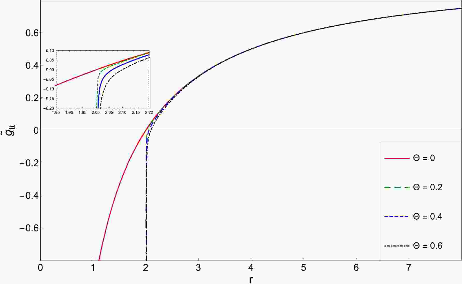
$ r_{\rm H}=2m $ is the event horizon of the Schwarzschild black hole in commutative space-time.As is clear from Fig. 1, the event horizon in the NC space-time is larger than that in the commutative space,
$ r_{\rm H}^{\rm NC}>r_{\rm H}^{\rm C} $ , where the singularity of the Schwarzschild solution at$ r=0 $ is now shifted by the non-commutativity of space to the finite radius,$ r=2m $ . Thus, the NC structure of space-time gives a non-singular black hole. This is a new result and is in contrast to the works published in Refs. [52, 56, 57] or in the theory of non-singularity black holes where the non-commutativity eliminates the point-like gravitational source [41–45], the Hayward black hole [58–61]. However, it agrees with the results of the quantum-corrected black hole theory [62–64], but just in the particular case where$ a=r_{\rm H} $ , with a in this theory being a minimal distance expected to be on the order of the Planck length,$ l_{\rm P} $ . The result is obtained when the singularity of the black hole in this theory is shifted to$ r=a=r_{\rm min}\sim l_{\rm P} $ ; hence, it is not a natural result because one would need to fix the parameter, a, for a particular value in order to observe the same result as in Fig 1. This is contrary to our results, which emerge naturally from the quantum structure of space-time itself when we impose the NC property of the geometry to space-time, without the need to impose a particular value to the NC parameter, Θ. Then, we conclude that the NC geometry removes the singularity at the origin of the black hole and increases the radius of the event horizon.
Figure 1. (color online) Behaviors of
$ \tilde{g}_{tt} $ for a stationary observer at spatial infinity in the non-commutative space-time with a given Θ.The corresponding Lagrangian can be written according to the non-commutative spacetime structure described by (45) as follows
$ 2L=\tilde{g}_{tt}(r,\Theta)c^{2}\dot{t}^{2}+\tilde{g}_{rr}(r,\Theta)\dot{r}^{2}+\tilde{g}_{\phi\phi}(r,\Theta)\dot{\phi}^{2} \,, $

(51) where the dots represent the derivative with respect to the affine parameter, τ, along the geodesic. Using the Euler-Lagrange equation
$ \begin{equation} \frac{\rm d}{{\rm d}s}\left(\frac{\partial L}{\partial \dot{x}^{\mu}}\right)-\frac{\partial L}{\partial x^{\mu}}=0\,, \end{equation} $

(52) and using the fact that L is independent of t and ϕ, we obtain two conserved quantities
$ E_{0}=p_{t}=c^{2}\tilde{g}_{tt}(r,\Theta)\dot{t}\Rightarrow \dot{t}=\frac{E_{0}}{c^{2}\tilde{g}_{tt}(r,\Theta)} \,, $

(53) $ l=p_{\phi}=\tilde{g}_{\phi\phi}(r,\Theta)\dot{\phi}\Rightarrow \dot{\phi}=\frac{l}{\tilde{g}_{\phi\phi}(r,\Theta)} \,. $

(54) Using the invariance① of
$ \tilde{g}_{\mu\nu}U^{\mu}U^{\nu}\equiv -h $ , together with relations (53) and (54), we obtain the explicit relation for$ \dot{r}^{2} $ $ \begin{equation} \dot{r}^{2}=-\frac{E_{0}^{2}}{c^{2}\tilde{g}_{tt}(r,\Theta)\tilde{g}_{rr}(r,\Theta)}-\frac{1}{\tilde{g}_{rr}(r,\Theta)}\left(\frac{l^{2}}{\tilde{g}_{\phi\phi}(r,\Theta)}+hc^{2}\right) \,, \end{equation} $

(55) where we shall consider
$ h=m_{0}^{2} $ for massive particles.Substituting (46), (47), and (49) into (55), and expanding in Θ up to
$ {\cal{O}}(\Theta^{3}) $ , equation (55) can be written as$ \begin{equation} \dot{r}^{2}+V_{\mathrm{eff}}(r,\Theta)=0 \,, \end{equation} $

(56) where
$ \begin{aligned}[b] V_{\mathrm{eff}}(r,\Theta)=&\left(1-\frac{2 m}{r}\right)\left(\frac{l^{2}}{r^{2}}+hc^{2}\right)-E^2+\Theta^{2}\left\{-\frac{l^{2}}{r^{4}}\left(\frac{5}{8}-\frac{3}{8}\sqrt{1-\dfrac{2m}{r}}+\frac{m\left(-17+{5}/{\sqrt{1-\dfrac{2m}{r}}}\right)}{16r}\right.\right.\\ &\left.\left.+\frac{m^2\sqrt{1-\dfrac{2m}{r}}}{(-2m+r)^2}\right)+E^{2}\left(\frac{m\left(64m^2+m\left(-49+13\sqrt{1-\dfrac{2 m}{r}}\right)r+2\left(13-3\sqrt{1-\dfrac{2 m}{r}}\right)r^2\right)}{16r^5\left(1-\dfrac{2m}{r}\right)^2}\right)\right.\\ &\left.+\left(\frac{l^{2}}{r^{2}}+hc^{2}\right)\left(\frac{m\left(12m^2+m\left(-14+\sqrt{1-\dfrac{2 m}{r}}\right)r-\left(5+\sqrt{1-\dfrac{2 m}{r}}\right)\right) r^2}{8r^5\left(1-\dfrac{2m}{r}\right)}\right)\right\}+{\cal{O}}(\Theta^{4}) \,. \end{aligned} $ 
(57) It is clear that when
$ \Theta\rightarrow 0 $ we restore the commutative effective potential for the Schwarzschild metric$ \begin{equation} V_{\mathrm{\mathrm{eff}}}(r,\Theta=0)=\left(1-\frac{2 m}{r}\right)\left(\frac{l^{2}}{r^{2}}+hc^{2}\right)-E^2\,. \end{equation} $

(58) We show in Fig. 2 the influence of the parameters Θ, m, E, and l on the effective potential for a massive particle. From this figure, we observe that, in the NC space-time, all the extremes of the effective potential are located outside the event horizon for any value of the used parameters. This deformed geometry adds a new minimum to this effective potential, which gives us multiple stable circular orbits. In Fig. 2(a), when Θ increases, the maximum peak of the curve decreases and shifts a little off the event horizon. We note here that the divergence around the event horizon is a consequence of the non-commutative geometry, which plays the role of a barrier preventing high-energy particles from falling into the event horizon. In Fig. 2(b), we observe that the increase of mass shifts the effective potential off the event horizon and increases the depth of the potential well in NC space-time. As we observe from Fig. 2(c), the effective potential depends on the energy of the test particle in NC space-time (57). Then, the increase in energy leads to an increase in the level of the effective potential and an increase in the depth of the potential well. For low-energy particles,
$ E\ll1 $ , the new minimum of the effective potential disappears and hence such particles fall into the event horizon. In Fig. 2(d), it is worth mentioning that in the NC space-time, there always exists a minimum of the effective potential near the event horizon whatever the value of the orbital momentum; when l increases, the depth of the potential well decreases and shifts towards the event horizon. The other extremes of the effective potential are restored when$ l_{\mathrm{crt}}>2\sqrt{3}\,\mathrm{m} $ .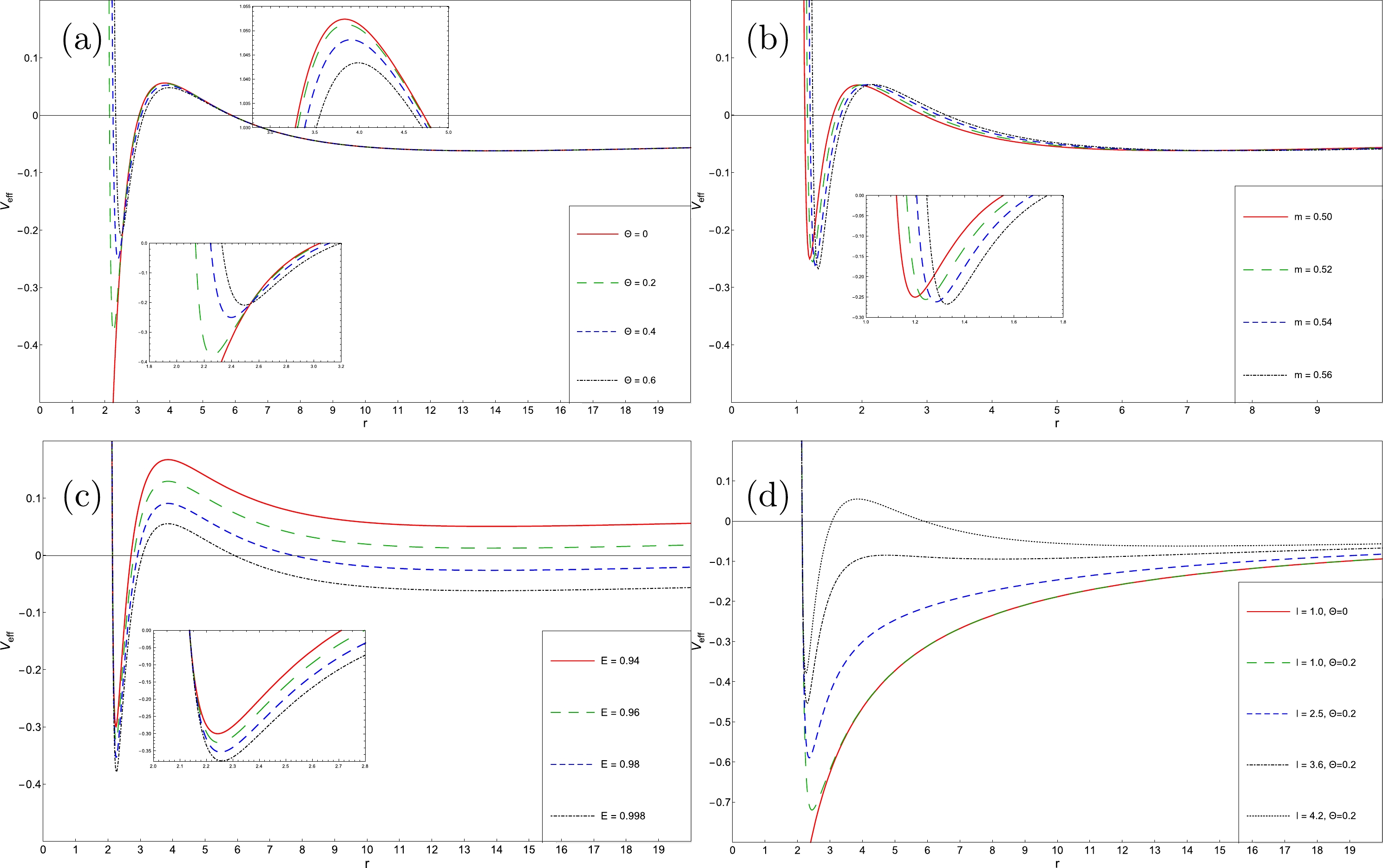
Figure 2. (color online) The behaviors of the effective potential for a massive particle. (a) different Θ and fixed:
$ E=0.998 $ ,$ m=1 $ ,$ l=4.2 $ . (b) different m and fixed:$ E=0.998 $ ,$ \Theta=0.2 $ , and$ l=4.2m $ . (c) different E and fixed:$ m=1 $ ,$ \Theta=0.2 $ , and$ l=4.2 $ . (d) different l and fixed:$ E=0.998 $ ,$ \Theta=0.2 $ , and$ m=1 $ .In this scenario, the NC geometry plays the role of the potential well near the event horizon when all matter absorbed by the black hole is compressed into this region before entering the event horizon. This leads to the formation of an accretion disk with high density and high temperature around the black hole, which becomes very bright. This is known as "Black Hole Accretion Disk Theory" (see Refs. [65–68]) and is also known in astronomy as "Quasar" (see Refs. [69, 70]).
The new minimum appearing in the behaviors of the effective potential in Fig. 2 can also be found in other theories such as Reissner-Norström charged black hole theory [71, 72], or the non-singularity black hole theory [60, 61]. While these theories have a problem with this minimum being located inside the event horizon and thus cannot be interpreted as a stable circular orbit, in our work, the non-commutativity shifts the new minimum outside of the event horizon, thus giving a possibility to a stable circular orbit near the event horizon. We elaborate on this in the following section.
-
In what follows, we treat the circular orbits and the stability condition in the NC space-time in order to see how the deformed geometry affects this class of orbits. For this, we take the case of circular orbits (
$ \dot{r}=0 $ ), where the corresponding effective potential must satisfy$ \begin{equation} V_{\mathrm{eff}}(r,\Theta)=V^{2}(r,\Theta)-E^{2}=0\,. \end{equation} $

(59) We can find the extreme of the non-commutative effective potential, given by the relation (57), in order to obtain the stable and unstable orbits, by solving the equation
$ \begin{equation} \frac{{\rm d}V_{\mathrm{eff}}}{{\rm d}r}=0\,. \end{equation} $

(60) In NC space-time, a minimum value of
$ V_{\mathrm{eff}} $ appears when$ l \geqslant 0, $ ② which corresponds to the Newtonian case. However, the existence of the maximum value of$ V_{\mathrm{eff}} $ requires a condition on the angular momentum, l, namely$ l_{\rm crt}> 2\sqrt{3}m $ . This corresponds to the relativistic case in commutative space-time. It is shown that the gravitational field gauge theory in NC Schwarzschild geometry using Seiberg-Witten maps is equivalent to the Newtonian case and the relativistic case in commutative Schwarzschild geometry.Table 1 shows the numerical solution of Eq. (60), representing the variation of the unstable and the multiple stable circular orbits as a function of the NC parameter Θ. The three types of circular orbits increase with increasing Θ. This behavior is represented in Fig. 3.
Θ 0 0.10 0.15 0.20 0.25 0.30 $r_{\rm sta}(\rm internal)$ 

2.16349 2.21421 2.25862 2.29837 2.33435 $r_{\rm uns}$ 

3.83278 3.83684 3.8419 3.84894 3.85791 3.86876 $r_{\rm sta}(\rm external)$ 

13.8072 13.8074 13.8076 13.8078 13.8081 13.8086 Table 1. Some numerical values for the unstable circular orbit,
$ r_{\rm uns} $ , and the multiple stable circular orbits,$ r_{\rm sta} $ , in the commutative and NC cases for different values of the parameter Θ and with the fixed values$ E=0.998,\; l=4.2,\; m=1 $ .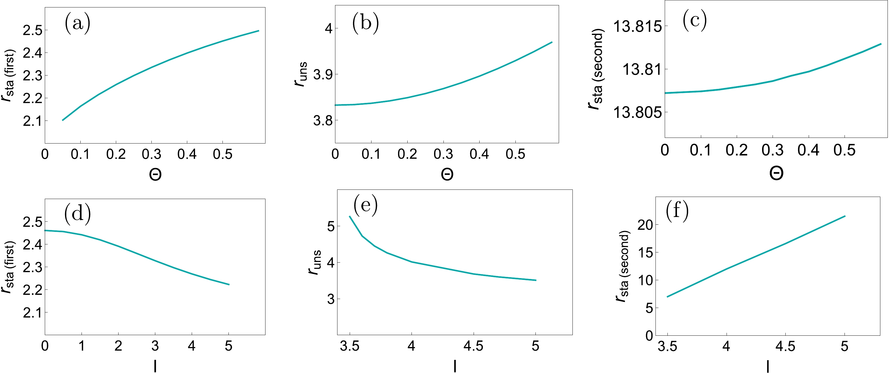
Figure 3. (color online) The behavior of the radius of the circular orbit for a particle in NC space-time. Unstable and multiple stable circular orbits as a function of Θ for fixed
$ l=4.2 $ ,$ E=0.998 $ , and$ m=1 $ in (a), (b), and (c) and as function of l for fixed$ \Theta=0.2 $ ,$ E=0.998 $ , and$ m=1 $ in (d), (e), and (f).We conclude from Fig. 3 that as the NC parameter, Θ, increases, all the types of radii increase in (a), (b), and (c). Therefore, the unstable circular orbital has a greater radius in NC space as the parameter increases, indicating a strong gravitational field. We also observe that when the angular momentum, l, increases, the unstable and internal stable circular orbits decrease, while the external stable circular orbit increases in (d), (e), and (f).
In astrophysics, the innermost stable circular orbit (ISCO) has a significant importance in describing the motion of a test body around a compact object. This class of orbits can be obtained from the stability condition given by
$ \begin{equation} \frac{{\rm d}^{2}V_{\mathrm{eff}}}{{\rm d}r^{2}}\geqslant 0 \,. \end{equation} $

(61) The numerical solution of these conditions show that
$r^{\rm C}_{\rm min}\geqslant 6$ in the commutative Schwarzschild space with$ l_{\rm crit} $ , and we obtain two conditions of stability orbits (see Fig. 4),$r_s \ll r^{\rm NC}_{\rm min} \leqslant 2.46729$ and$ r^{\rm NC}_{\rm min} \geqslant 6.00772 $ , for a NC Schwarzschild space using Seiberg-Witten maps with the parameter$ \Theta=0.2 $ , corresponding to multiple innermost stable orbits.
Figure 4. (color online) The condition for stability of circular orbits for different Θ and fixed other parameters: (a)
$ E=1 $ ,$ l_{\rm crit}=2\sqrt{3} $ , and$ m=1 $ . (b)$ E=1 $ ,$ l_{\rm crit}=\sqrt{3} $ , and$ m=0.5 $ . (c)$ E=1 $ ,$ l_{\rm crt}=6\sqrt{3}/14 $ , and$ m=3/14 $ .We show in Fig. 4 the behavior of the composite conditions given in Eqs. (60) and (61) for fixed E and for different values for the parameters
$ l_{\rm crit} $ , m, and Θ. As is clear from the figure in the commutative space, we have just one condition for the innermost stable circular orbit, while the NC space increases this condition for the innermost stable circular orbit and adds a new condition for the stable circular orbit near the event horizon of the static black hole. Another note that can be seen from the figure is that when the mass of the black hole decreases, the NC effect increases, suggesting that the NC correction term is proportional to$ 1/m $ .We show in Fig. 5 the behavior of the stability condition of circular orbits as a function of the mass, m, in (a) and as a function of the NC parameter, Θ, in (b). We notice that when the mass increases, the two stability conditions in the NC space-time increase, and similarly, when the NC parameter increases, these two stability conditions increase. From this behavior in Fig. 5, we can see that the NC parameter, Θ, plays the same role as the mass, m, and this can be used to explain dark matter in this universe.
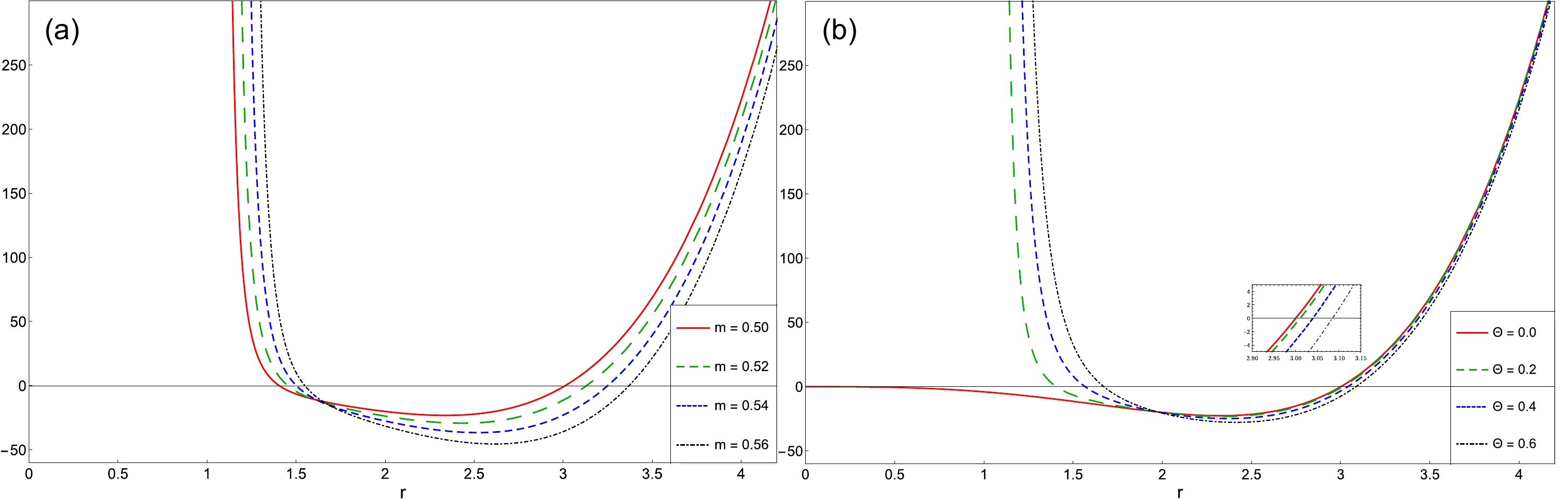
Figure 5. (color online) The condition for the stability of circular orbits for fixed
$ E=1 $ . (a) different m,$ l_{\rm crit}=2\sqrt{3} m $ , and fixed$ \Theta=0.2 $ . (b) different Θ and fixed$ m=0.50 $ .In Table 2 we show the numerical solutions that are obtained according to conditions given in Eqs. (60) and (61). Figure 4 represents the variation of the innermost stable circular orbit radius as function of Θ, which is found to increase with increasing Θ. We see here that the NC space predicts a new stable circular orbit near the event horizon, which is absent in the commutative space. This is shown in Fig 6.
Θ 0 0.10 0.15 0.20 0.25 0.30 $ r_{\rm (a)min} \geqslant $ 

6 6.00127 6.00286 6.00507 6.00792 6.01138 $ r_s \ll r_{\rm (a)min} \leqslant $ 

2.39118 2.48542 2.5655 2.63613 2.69974 $ r_{\rm (b)min} \geqslant $ 

3 3.00254 3.00569 3.01008 3.01566 3.02241 $ r_s \ll r_{\rm (b)min} \leqslant $ 

1.28275 1.34987 1.40569 1.45373 1.49587 $ r_{\rm (c)min} \geqslant $ 

1.28571 1.29157 1.29869 1.3083 1.32011 1.33377 $ r_s \ll r_{\rm (b)min} \leqslant $ 

0.616476 0.657125 0.688445 0.713273 0.733258 Table 2. Numerical solutions for the radius condition of the innermost stable circular orbit with different parameters Θ and fixed
$E=1,\quad l_{\rm crit}= 2\sqrt{3}m$ , and m. (a)$ m=1 $ , (b)$ m=0.5 $ , and (c)$ m=3/14 $ .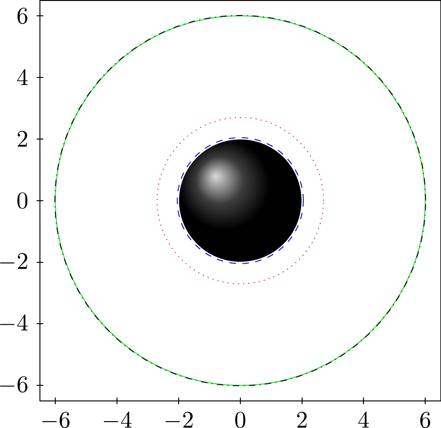
Figure 6. (color online) Position of the innermost stable circular orbit with
$ E=1 $ ,$ m=1 $ ,$ h=1 $ , and$l_{\rm crit}= 2\sqrt{3}$ . The circle with a solid line represents ISCO for the Schwarzschild black hole (black disk in center) in the commutative case,$ \Theta=0 $ . The dashed line represents the NC event horizon, the dot lines represent the new ISCO in internal region (near the event horizon), and the dot-dashed lines represents ISCO in external region for the Schwarzschild black hole in the NC case$ \Theta=0.3 $ .From the two Tables 1 and 2, we conclude that the NC space increases the radius of the stable circular orbits and adds a possibility of multiple stable circular orbits near the event horizon of a static black hole.
-
In order to obtain the analytic formula for the periastron advance, we need to obtain the equation of motion (56) as a function of ϕ. To achieve this, we use the angular momentum Eq. (54) to write
$ r=r(\phi) $ $ \begin{equation} \frac{{\rm d}r}{{\rm d}\tau}=\frac{{\rm d}r}{{\rm d}\phi}\frac{{\rm d}\phi}{{\rm d}\tau}=\frac{l}{\tilde{g}_{\phi\phi}(r,\Theta)}\frac{{\rm d}r}{{\rm d}\phi}\,. \end{equation} $

(62) We substitute this into Eq. (56), and we obtain
$ \begin{equation} \left(\frac{{\rm d}r}{{\rm d}\phi}\right)^{2}=-\frac{\tilde{g}_{\phi\phi}^{2}(r,\Theta)}{l^{2}}V_{\rm eff}(r,\Theta)\,, \end{equation} $

(63) where we use relations (56) and (57) in the case of a massive particle,
$ h=m_{0}^{2} $ .We define a new variable,
$ u={1}/{r} $ ; thus, we find$ \begin{aligned}[b] \left(\frac{{\rm d}u}{{\rm d}\phi}\right)^{2}=&\frac{(E^{2}-m_{0}^{2}c^{2})}{l^2}+\frac{2mm_{0}^{2}c^{2}}{l^{2}}u-u^2+2mu^3-\Theta^{2}\left\{-u^4(1-2mu)\left(\frac{5}{8}-\frac{3}{8}\sqrt{1-2mu}\right.\right.\left.+\frac{1}{16}mu\left(-17+\frac{5}{\sqrt{1-2mu}}\right)+\frac{m^2u^2}{(1-2mu)^{\frac{3}{2}}}\right)\\ &-\frac{2u^2}{l^2}\left(E^2+(-1+2mu)(m_{0}^{2}c^{2}+l^2u^2)\right) \left.\times\left(\frac{5}{8}-\frac{3}{8}\sqrt{1-2mu}+\frac{1}{16}mu\left(-17+\frac{5}{\sqrt{1-2mu}}\right)+\frac{m^2u^2}{(1-2mu)^{\frac{3}{2}}}\right)\right.\\ &\left.+\left(\frac{E^{2}mu^3(64u^2m^2+mu(-49+13\sqrt{1-2mu})+2(13-3\sqrt{1-2mu}))}{16l^{2}(1-2mu)^2}\right)\right.\\ &\left.+\frac{mu^3(m_{0}^{2}c^{2}+l^2u^2)(12u^2m^2+mu(-14+\sqrt{1-2mu})-(5+\sqrt{1-2mu}))}{8 l^2 (1-2mu)}\right\}+{\cal{O}}(\Theta^{4})\,. \end{aligned} $

(64) Using the fact that
$ mu\ll 1 $ , we rewrite the above equation in a linear form stopping at 3$ ^{\mathrm{rd}} $ order in u, and hence, we find$ \begin{aligned}[b] \left(\frac{{\rm d}u}{{\rm d}\phi}\right)^{2}=&\frac{(E^{2}-m_{0}^{2}c^{2})}{l^2}+\frac{2mm_{0}^{2}c^{2}}{l^{2}}u-u^2+2mu^3\\&+\frac{\Theta^{2}}{2l^2}\left\{(E^2-m_{0}^{2}c^{2})u^2+m(5m_{0}^{2}c^{2}-4E^{2})u^3\right\}.\end{aligned} $

(65) Taking the derivative of the above equation with respect to ϕ yields
$ \begin{aligned}[b] \frac{{\rm d}^{2}u}{{\rm d}\phi^{2}}+u=&\frac{mm_{0}^{2}c^{2}}{l^{2}}+3mu^{2}+\frac{\Theta^{2}}{2l^2}\Bigg\{(E^2-m_{0}^{2}c^{2})u\\&+\frac{3m}{2}(5m_{0}^{2}c^{2}-4E^{2})u^2\Bigg\}\,, \end{aligned} $

(66) which is the non-commutative geodesic equation.
In Fig. 7, we plot the geodesic Eq. (65) for a massive particle around a NC Schwarzschild Black Hole, for different values of l and E and with a fixed black hole mass,
$ m=3/14 $ . As is clear from (a) and (b), the non-commutativity of space-time decreases the major semi-axis of the particle orbit, which remains stable. This signifies that the NC effects are responsible for increasing the strength of the gravitational field.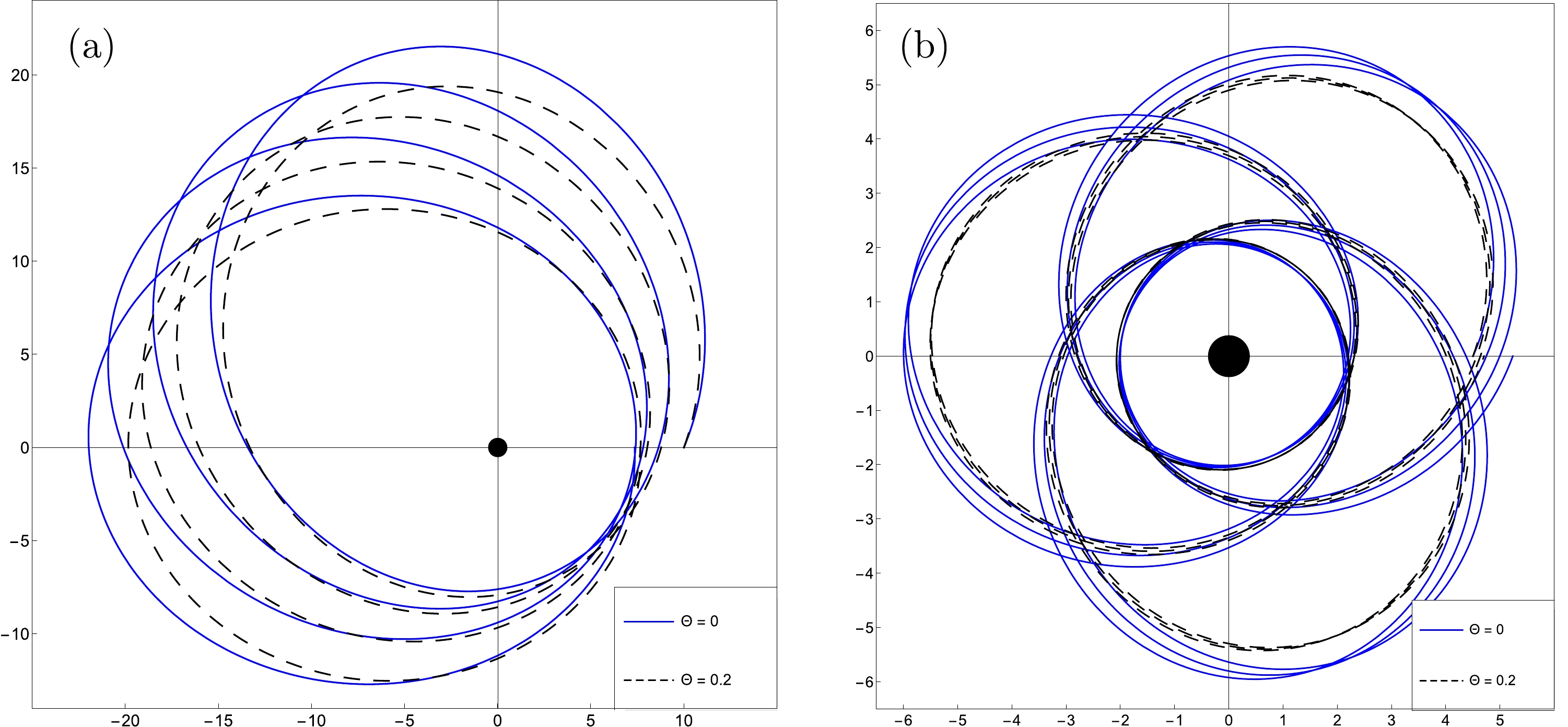
Figure 7. (color online) Time-like geodesic for a test particle,
$ h=1 $ , around a non-commutative Schwarzschild Black-Hole with different values of Θ and for fixed values of the parameters in the plane$\theta={\pi}/{2}$ : (a)$ M={3}/{14} $ ,$ l=1.586 $ , and$ E=0.993 $ . (b)$M={3}/{14}$ ,$ l=0.915 $ , and$ E=0.975 $ . -
Let us write this equation into perturbation form of the Keplerian trajectory equation
$ \begin{equation} \frac{{\rm d}^{2}u}{{\rm d}\phi^{2}}+u=\frac{m}{\tilde{l}^{2}}+\frac{g(u)}{\tilde{l}^{2}}\,, \end{equation} $

(67) where
$ \tilde{l}=\dfrac{l}{m_{0}c} $ , and$ g(u)=3mu^{2}+\dfrac{\Theta^{2}}{2l^2}\Bigg\{(E^2-m_{0}^{2}c^{2})u+ \dfrac{3m}{2} \times (5m_{0}^{2}c^{2}-4E^{2})u^2\Bigg\}. $

Following the same steps as in Ref. [73], we obtain the deviation angle after one revolution
$ \begin{equation} \Delta\phi=\frac{\pi g_{1}}{\tilde{l}^{2}} \,, \end{equation} $

(68) where
$ g_{1}=\dfrac{{\rm d}g(u)}{{\rm d}u}\Big|_{u={1}/{b}} $ , and the distance, b, is defined by$ b=m\alpha(1-e^{2}) $ , with α and e denoting the major semi-axis and the eccentricity of the movement. Using relation (68), we find the deviation angle in the NC space$ \begin{aligned}[b] \Delta\phi=&\frac{6\pi GM}{c^{2}\alpha (1-e^{2})}+\pi\Theta^{2}\Bigg[\frac{(E^{2}_0/c^{2}-m^{2}_{0}c^{2})}{2m\alpha(1-e^{2})}\\&+\frac{6(m^{2}_{0}c^{2}-E^{2}_0/c^{2})}{\alpha^{2}(1-e^{2})^{2}}+\frac{3m^{2}_{0}c^{2}}{2\alpha^{2}(1-e^{2})^{2}}\Bigg]\,. \end{aligned} $

(69) We have thus found a result that is quite close to that found in Ref. [40], where just the star product was used, while in our work, we used the Seiberg-Witten map. Using the relativistic relation of dispersion, we find
$ \begin{aligned}[b] \Delta\phi=&\frac{6\pi GM}{c^{2}\alpha (1-e^{2})}+\pi\Theta^{2}\Bigg[\frac{m^{2}_{0}v^{2}c^{2}}{2GM\alpha(1-e^{2})}\\&-\frac{6m^{2}_{0}v^{2}}{\alpha^{2}(1-e^{2})^{2}}+\frac{3m^{2}_{0}c^{2}}{2\alpha^{2}(1-e^{2})^{2}}\Bigg]\,. \end{aligned} $

(70) It is clear that the first term represents the well-known predictions of general relativity, as well as a correction that is dependent on the NC parameter.
For a numerical application, we take the case of the planet Mercury. We find that the NC perihelion shift is given by
$ \begin{equation} \mid\delta \phi_{\rm NC}\mid=\left(1.96689\times10^{43}\right)\Theta^{2}{\rm Kg^{2}\cdot s}^{-2}\,. \end{equation} $

(71) The general relativity prediction and the observed perihelion shift for Mercury are given in Ref. [74] by
$ \delta \phi_{\rm obs}=2\pi\left(7.98734\pm0.00037\right)\times10^{-8}\rm\ rad/rev\,, $

(72) $ \delta \phi_{\rm GR}=2\pi\left(7.98742\right)\times10^{-8}\rm\ rad/rev\,. $

(73) Comparing the NC correction to the observable data (
$ \mid\delta \phi_{\rm NC}\mid\approx \delta \phi_{\rm obs} $ ), we estimate the value of Θ to be$ \begin{equation} \Theta\approx 1.597 \times 10^{-25} {\rm s\cdot Kg}^{-1}\,, \end{equation} $

(74) or equivalently
$ \begin{equation} \sqrt{\hbar\Theta} \approx 1.029 \times 10^{-29} {\rm m}\,. \end{equation} $

(75) We can then define a lower bound for Θ using
$ \mid\delta \phi_{\rm NC} \mid\;\leq \;\mid \delta \phi_{\rm GR}-\delta \phi_{\rm obs}\mid\;\approx 2\pi(1\times10^{-12})\rm\ rad/rev\,. $

(76) Thus, we get
$ \begin{equation} \Theta\leq 5.0553 \times10^{-28}{\rm s\cdot kg}^{-1}\,, \end{equation} $

(77) or equivalently
$ \begin{equation} \sqrt{\hbar\Theta}\leq 5.7876 \times10^{-31}{\rm m}\,. \end{equation} $

(78) It is clear that the NC parameter, Θ, is very small, and it is remarkable that our result is very close to that obtained in Refs. [37, 38], where classical mechanics in NC flat space is used. We note that our result has a difference on the order of
$ 10^{-1} $ relative to the result obtained in Ref. [38], which occurs because we used a curved space-time. Furthermore, the result of Ref. [37] includes a new degree of freedom, γ, and for the specific value of γ used therein, one obtains the same result as ours. This result leads us to the same conclusion arrived at in Ref. [38], that planetary systems are very sensitive to the NC parameter. In this way the NC parameter plays the role of a fundamental constant of the system to describe the microstructure of space-time in this region. Thus any small change in Θ implies a sensible change to our system at a large scale.Comparing our result with the Planck length, we find
$ \sqrt{\hbar\Theta}>L_{\rm P} $ . The NC parameter also has a lower bound, which is the Planck scale,$ L_{\rm P} $ $ \begin{equation} \sqrt{\hbar\Theta}\leq (3.5808 \times10^{4})L_{\rm P}\,. \end{equation} $

(79) Using natural units, we obtain the upper bound of the energy
$ \begin{equation} 3.39 \times 10^{14}{\rm GeV} \leq \frac{1}{\sqrt{\hbar\Theta}}\,, \end{equation} $

(80) which also has an upper bound given by Planck energy
$ E_{\rm P} $ . -
In this study, we investigated the geodesic motion of a test particle in NC Schwarzschild space-time. By using the Seiberg-Witten map and a general form of the tetrad field for the Schwarzschild black hole, we showed that all the non-zero components of the deformed metric,
$ \tilde{g}_{\mu\nu}(r,\Theta) $ , acquire a singularity in the NC correction term at the value$ r=2m $ , which are absent in Ref. [52]; this singularity in the component$ \tilde{g}_{00} $ removes the singularity at the origin,$ r=0 $ , of the black hole. This result emerged naturally from the NC structure of space-time, itself. We then obtained a non-singular black hole and we showed that the event horizon in NC space-time is bigger than in the commutative case,$ r^{\rm NC}_{\rm H}>r^{\rm C}_{\rm H} $ ; thus, the Schwarzschild radius plays the role of the radius of the compact object inside the NC black hole.The NC effective potential of the particles in the NC Schwarzschild space-time was calculated and through detailed analysis, new stable circular orbits appear near the event horizon. Therefore, the geodetic structure of this black hole presents new types of motion next to the event horizon within stable orbits that are not allowed by Schwarzschild space-time. This difference around the event horizon is a result of the non-commutative geometry, which acts as a barrier to prevent particles from falling into the event horizon. As in NC space-time, the commutativity parameter plays the same role as the mass of black hole, which can be used to explain dark matter.
Finally, we found that the NC space-time decreases the major semi-axis of the particles orbit. This indicates that the effects of the non-commutativity increase the strength of the gravitational field. Then, we obtained the NC periastron advance of Mercury's orbit and compared it with experimental data to obtain a value for the Θ parameter on the order of
$10^{-25}\,\mathrm{s\cdot kg}^{-1}$ , which gives observable deviation in the perihelion shift of Mercury. The lower bound to$ \sqrt{\hbar\Theta} $ shows that the NC propriety appears before the Planck length scale. However, for a better comparison, it will be necessary to study in a non-commutative curved space with the presence of torsion.
Geodesic equation in non-commutative gauge theory of gravity
- Received Date: 2022-05-13
- Available Online: 2022-10-15
Abstract: In this study, we construct a non-commutative gauge theory of the modified structure of the gravitational field using the Seiberg-Witten map and the general tetrad fields of Schwarzschild space-time to show that the non-commutative geometry removes the singularity at the origin of the black hole, thus obtaining a non-singular Schwarzschild black hole. The geodetic structure of this black hole presents new types of motion next to the event horizon within stable orbits that are not allowed by the ordinary Schwarzschild spacetime. The noncommutative periastron advance of the Mercury orbit is obtained, and with the available experimental data, we find a parameter of non-commutativity on the order of


 DownLoad: