


 Abstract
 HTML
HTML Reference
 Related
 PDF
PDF


-
According to the global fits to neutrino oscillation data [1], it is well known that the three mixing angles in the lepton sector are close to the tribimaximal (TBM) mixing [2–4]. In the TBM pattern, the values of the three mixing angles are as follows:
$ \sin^2\theta_{12}={1}/{3} $ ,$ \sin^2\theta_{23}={1}/{2} $ , and$ \sin^2\theta_{13}=0 $ . In contrast, the$C P$ violating Dirac phase,$ \delta_{ CP} $ , in the lepton sector is yet to be measured precisely. However, from the global fits to neutrino oscillation data [1], the best fit value for$ \delta_{CP} $ is around$\pi({3}/{2}\pi)$ in the case of normal (inverted) ordering of neutrino masses. The TBM value for$ \theta_{23} $ and$ \delta_{CP}=({3}/{2})\pi $ are still allowed in the$ 3\sigma $ ranges for these observables in the current neutrino oscillation data [1]. The aforementioned values for$ \theta_{23} $ and$ \delta_{CP} $ are considered to be maximal. To explain these maximal values forθ23 and δCP, Harrison and Scott have proposed the$ \mu-\tau $ symmetry in combination with${C P}$ symmetry, together called$ \mu-\tau $ reflection symmetry [5]. For further works regarding the$ \mu-\tau $ and${ C P}$ symmetries, see Refs. [6–12]. Ref. [6] is a review article.In the work by Grimus and Lavoura [13], it is shown that a mass matrix for light left-handed neutrinos has the following form [14]:
$ \begin{equation} {\cal M}_\nu=\left(\begin{array}{ccc} a & r & r^* \\ r & s & b \\ r^* & b & s^* \end{array}\right) \end{equation} $

(1) which can yield maximal values for
$ \theta_{23} $ and$ \delta_{CP} $ . In the above equation,$ a,b $ are real and$ r,s $ are complex. Further, in Ref. [13], a model is constructed, which is based on$ \mu-\tau $ reflection symmetry and softly broken lepton numbers, to obtain a mass matrix of the same form as in Eq. (1) for light neutrinos. In this model, three Higgs doublets are introduced and light neutrinos acquire masses via type I seesaw mechanism [15, 16]. The lepton number is softly broken by the mass terms for right-handed neutrinos in this model. However, in the absence of parameter fine tuning in the model, muon and tau leptons can have masses of the same order. To explain the hierarchy in the masses for these leptons, K symmetry is introduced, under which the muon is massless [13]. Realistic masses for muon and tau leptons are explained in the above mentioned scenario with the soft breaking of the K symmetry [17]. The work done together in Refs. [13, 17], which is based on$ \mu-\tau $ reflection symmetry, consistently explains the mixing pattern in lepton sector and also the masses for charged leptons.Although the work done in Refs. [13, 17] gives a consistent picture about masses and mixing pattern in the lepton sector, it suffers from a few limitations, as explained below. It is argued in Ref. [13] that the mass matrix of Eq. (1), which is obtained from
$ \mu-\tau $ reflection symmetry, cannot give predictions about neutrino mass ordering and the mixing angle$ \theta_{12} $ . Moreover, in the case of maximal$ \delta_{CP} $ , the mass matrix of Eq. (1) can make no predictions regarding$ \theta_{13} $ [13]. From the current neutrino oscillation data, it is known that neutrinos can have either normal or inverted mass ordering, where$ \sin^2\theta_{12}\sim{1}/{3} $ and$ \sin^2\theta_{13}\sim10^{-2} $ [1]. Apart from the above mentioned limitations, in Ref. [13], mixing pattern in the quark sector was not addressed. Nonetheless, the mixing pattern in the quark sector [18] is known to be different from that of lepton sector. The interest would be to know whether the same framework could be used to understand the mixing patterns for both quark and lepton sectors.As stated above, in Ref. [13], a model, which is based on type I seesaw mechanism and
$ \mu-\tau $ reflection symmetry, is presented with the aim of obtaining the neutrino mass matrix of the same form as Eq. (1). In this work, we rather aim at investigation whether the matrix in Eq. (1) can be obtained with type II seesaw mechanism [19–21] in the framework of$ \mu-\tau $ reflection symmetry. To achieve this, we construct a model, which has three Higgs doublets and one scalar Higgs triplet. In our model, right-handed neutrinos do not exist, and hence, neutrinos acquire masses when the Higgs triplet get vacuum expectation value (VEV). The purpose of Higgs doublets is to give masses to charged leptons via Yukawa couplings. With the$ \mu-\tau $ reflection symmetry in our model, if the VEV of Higgs triplet is real, we show that mass matrix for the light neutrinos will have the form of Eq. (1). To show whether the VEV of the Higgs triplet could be real, we analyze the scalar potential of our model. We demonstrate that by using an extra discrete symmetry, the VEV of Higgs triplet can be real. In parallel to that, we also address the problem of hierarchy in the masses of muon and tau leptons. In the literature, models have been constructed in order to achieve maximal values for$ \theta_{23} $ and$ \delta_{CP} $ using type II seesaw mechanism [22, 23]. However, in these models, multiple Higgs triplets have been introduced in addition to the three Higgs doublets. Hence, our model proposed here is economical compared to the aforementioned models.As stated previously, the mass matrix form given in Eq. (1) can predict maximal values for
$ \theta_{23} $ and$ \delta_{CP} $ . However, this matrix cannot make predictions about neutrino mass ordering and the mixing angles$ \theta_{12},\theta_{13} $ . As already pointed before, we have$ \sin^2\theta_{13}\sim10^{-2} $ [1], which means that$ \theta_{13} $ is a small angle. In this work, we perform an analysis, based on approximation procedures [24, 25], and derive some conditions on the elements of neutrino mass matrix which can make predictions about the neutrino mass ordering and smallness of$ \theta_{13} $ , apart from giving maximal values for$ \theta_{23} $ and$ \delta_{CP} $ . In this analysis, we assume$ \sin^2\theta_{12}\sim{1}/{3} $ . To achieve the above mentioned conditions, new mechanisms should be proposed. In this work, we have attempted to provide one mechanism to achieve one of those conditions.In our model three Higgs doublets give masses to charged leptons. Thus, it is worth knowing whether these scalar doublets can also generate masses and mixing pattern for quarks. Due to
$ CP $ symmetry in the lepton sector, it is found that these Higgs doublets should transform non-trivially under the$ CP $ symmetry. As a result, we propose$ CP $ transformations for quarks in such a way that the corresponding Yukawa couplings are invariant under the$ CP $ symmetry. A large hierarchy among the masses of quarks is known. Hence, to explain the mixing pattern for quarks, their Yukawa couplings should be hierarchically suppressed [26]. To explain the realistic mixing pattern for quarks through hierarchically suppressed Yukawa couplings, we followed the work done in Refs. [27, 28]. For more information regarding other works on quark and lepton mixings with generalized$ CP $ transformations, see Ref. [29, 30]. Additional works addressing quark and lepton mixings with other symmetries could be found in Refs. [31–33].The paper is organized as follows. In the next section, we propose a model for lepton mixing, where maximal values for
$ \theta_{23} $ and$ \delta_{CP} $ can be predicted if the VEV of triplet Higgs is real. In Sec. III, we analyze the scalar potential of our model and show that the VEV of triplet Higgs can be real if we introduce additional discrete symmetry$ Z_3 $ . In Sec. IV, we obtain some conditions on the elements of the neutrino mass matrix of our model, which enable predictions about the neutrino mass ordering and smallness of$ \theta_{13} $ . In Sec. VI, we investigate quark masses and mixing patterns and demonstrate that they can be explained in the framework of our model. Conclusions are presented in the last section. In the Appendix, we attempt to describe a mechanism for achieving normal order of neutrino masses. -
The model we propose for lepton mixing is similar to that in Ref. [13]. We propose scalar Higgs doublets
$ \phi_i=(\phi_i^+,\phi_i^0)^T $ , where$ i=1,2,3 $ , in order to give masses to charged leptons. We denote the lepton doublets and singlets by$ D_{\alpha {\rm L}}=(\nu_{\alpha {\rm L}},\alpha_{\rm L})^T $ and$ \alpha_R $ , where$ \alpha=e,\mu,\tau $ , respectively. The$ CP $ transformations on the lepton fields and Higgs doublets are defined as [13]$ \begin{aligned}[b] & D_{\alpha {\rm L}}\to {\rm i}S_{ \alpha\beta}\gamma^0C\bar{D}_{\beta {\rm L}}^T,\quad \alpha_{\rm R}\to {\rm i}S_{ \alpha\beta}\gamma^0C\bar{\beta}_{\rm R}^T, \\& S=\left(\begin{array}{ccc} 1 & 0 & 0 \\ 0 & 0 & 1 \\ 0 & 1 & 0 \end{array} \right), \quad \phi_{1,2}\to\phi_{1,2}^*,\quad \phi_3\to -\phi_3^*. \end{aligned} $

(2) Here, C is the charge conjugation matrix. In addition to the invariance under the above mentioned
$C P$ transformations, one needs to impose conservation of$ U(1)_{L_\alpha} $ and$ Z_2 $ symmetries. Here,$ U(1)_{L_\alpha} $ is the lepton number symmetry for the individual family of leptons. Under$ Z_2 $ symmetry, only the$ e_{\rm R} $ and$ \phi_1 $ change sign. Considering the aforementioned charge assignments, the invariant Lagrangian for charged lepton Yukawa couplings is given by [13]$ \begin{equation} {\cal L}_{\rm Y} = -y_e\bar{D}_{e{\rm L}}\phi_1e_{\rm R}-\sum\limits_{j=2}^3\sum\limits_{\alpha=\mu,\tau} g_{j\alpha}\bar{D}_{\alpha {\rm L}}\phi_j\alpha_{\rm R} +{\rm h.c}.. \end{equation} $

(3) In order for the Lagrangian in Eq. (3) to be invariant under
$C P$ symmetry, we should have$ y_e $ to be real,$ g_{2\mu}=g_{2\tau}^* $ and$ g_{3\mu}=-g_{3\tau}^* $ . Since the mass of electron should be real, we take the VEV of$ \phi_1 $ to be real. In contrast, the VEVs of$ \phi_{2,3} $ should be complex, which give masses to muon and tau leptons, whose forms are given below [13].$ \begin{equation} m_\mu=|g_{2\mu}v_2+g_{3\mu}v_3|,\quad m_\tau=|g^*_{2\mu}v_2-g^*_{3\mu}v_3|. \end{equation} $

(4) In this work, we take
$ \langle\phi_i^0\rangle=v_i $ for$ i=1,2,3 $ . As an a priori assumption, the VEVs of all Higgs doublets are of the same order. Hence, from the above equations, we notice that some fine tuning is necessary in order to explain the hierarchy in the muon and tau lepton masses. To reduce this fine tuning, K symmetry is introduced, under which the non-trivial transformations of the fields are given below [13]$ \begin{equation} \mu_R\to -\mu_R,\quad \phi_2\leftrightarrow\phi_3. \end{equation} $

(5) After imposing this K symmetry in the above model, one can see that
$ g_{2\mu}=-g_{3\mu} $ . Using this in Eq. (4), we get$ \begin{equation} \frac{m_\mu}{m_\tau}=\left|\frac{v_2-v_3}{v_2+v_3}\right|. \end{equation} $

(6) Since the scalar potential of this model should also respect the K symmetry, we should get
$ v_2=v_3 $ , and hence,$ m_\mu=0 $ . Now, to explain a non-zero but small$ m_\mu $ , soft breaking of K symmetry can be introduced into the scalar potential of this model [17]. The analysis related to this is presented in the next section.To explain the masses for neutrinos in the above described framework, we introduce the following Higgs triplet into the model.
$ \begin{equation} \Delta=\left(\begin{array}{cc} \dfrac{\Delta^+}{\sqrt{2}} & \Delta^{++} \\ -\Delta^0 & -\dfrac{\Delta^+}{\sqrt{2}} \end{array}\right). \end{equation} $

(7) Δ is singlet under
$ Z_2 $ , but otherwise transform under$C P$ symmetry as$ \Delta\to\Delta^* $ . Now, the Yukawa couplings for neutrinos can be written as$ \begin{equation} {\cal L}_Y=\frac{1}{2}\sum\limits_{\alpha,\,\beta=e,\,\mu,\,\tau}Y^\nu_{\alpha\beta} \bar{D}^c_{\alpha {\rm L}}{\rm i}\sigma_2\Delta D_{\beta {\rm L}}+{\rm h.c}.. \end{equation} $

(8) Here,
$ D_{\alpha {\rm L}}^c $ is the charge conjugated doublet for$ D_{\alpha {\rm L}} $ , and$ \sigma_2 $ is a Pauli matrix. We can notice that the terms in the above Lagrangian break the lepton number symmetry$ U_{L_\alpha} $ explicitly. This can be considered technically natural, since the neutrino masses become zero in this model in the limit that the symmetry$ U_{L_\alpha} $ is exact. Hence, to explain the smallness of neutrino masses, the symmetry of$ U_{L_\alpha} $ can be broken by small amounts. Therefore, here, the neutrino Yukawa couplings$ Y^\nu_{\alpha\beta} $ can be small. Due to the invariance under$C P$ symmetry, these Yukawa couplings should satisfy$ \begin{equation} SY^\nu S=(Y^\nu)^*. \end{equation} $

(9) After electroweak symmetry breaking, we can have
$ \langle\Delta^0\rangle=v_\Delta $ . Now, from Eq. (8), we get the mass matrix for neutrinos, which is given by$ M_\nu=Y^\nu v_\Delta $ . If$ v_\Delta $ is real, using Eq. (9), we get$ \begin{equation} SM_\nu S=M_\nu^*. \end{equation} $

(10) In order to satisfy the above relation, the form for
$ M_\nu $ should be the same as in Eq. (1). Hence, in the above proposed model, the mixing angle$ \theta_{23} $ and the$C P$ violating phase$ \delta_{CP} $ are maximal. However, to satisfy the relation in Eq. (10),$ v_\Delta $ should be real. In the next section, we present an analysis of the scalar potential in our model, where we demonstrate that$ v_\Delta $ can be real.Now, we estimate the value of
$ v_\Delta $ in our work. As stated above, the neutrino mass matrix is$ M_\nu=Y^\nu v_\Delta $ . Since the couplings$ Y^\nu $ should be small, because they break the$ U_{L_\alpha} $ symmetry by a small amount, we take$ Y^\nu\sim 10^{-3} $ . Now, by fitting$ M_\nu $ to neutrino masses, which are obtained from the neutrino oscillation data, an estimation of$ v_\Delta $ can be obtained. Using the neutrino oscillation data, the following mass-square differences have been found [1], where we have given the best fit values.$ \begin{aligned}[b]& m_s^2\equiv m_2^2-m_1^2=7.5\times10^{-5}\; {\rm eV}^2,\\& m_a^2\equiv\left\{\begin{array}{c} m_3^2-m_1^2=2.55\times10^{-3}\; {\rm eV}^2\; \; {\rm (NO)}\\ m_1^2-m_3^2=2.45\times10^{-3}\; {\rm eV}^2\; \; {\rm (IO)} \end{array}\right.. \end{aligned} $

(11) Here,
$ m_{1,2,3} $ are neutrino mass eigenvalues and NO(IO) represents normal (inverted) ordering. Using the above values, we get$ m_s\sim0.0087 $ eV and$ m_a\sim0.05 $ eV, which correspond to solar and atmospheric neutrino mass scales, respectively. To fit these neutrino mass scales in our work, we can take$ v_\Delta\sim1-10 $ eV. -
The scalar fields of the model proposed in the previous section are charged under the symmetry
$ C P\times Z_2\times K $ . The invariant scalar potential of this model can be written as$ \begin{equation} V_{\rm inv}=V_D+V_T. \end{equation} $

(12) Here,
$ V_D $ contains potential terms only for the Higgs doublets.$ V_T $ is the scalar potential for the triplet Higgs in our model. The form of$ V_D $ is given by [17]$ \begin{aligned}[b] V_D=& -M_1^2\phi_1^\dagger\phi_1 -M_2^2(\phi_2^\dagger\phi_2+\phi_3^\dagger\phi_3) +\lambda_1(\phi_1^\dagger\phi_1)^2 \\&+\lambda_2\left[(\phi_2^\dagger\phi_2)^2+(\phi_3^\dagger\phi_3)^2\right] \\ &+\lambda_3(\phi_1^\dagger\phi_1)(\phi_2^\dagger\phi_2+\phi_3^\dagger\phi_3) +\lambda_4(\phi_2^\dagger\phi_2)(\phi_3^\dagger\phi_3) \\&+\lambda_5\left[(\phi_1^\dagger\phi_2)(\phi_2^\dagger\phi_1) +(\phi_1^\dagger\phi_3)(\phi_3^\dagger\phi_1)\right] \\ &+\lambda_6\left[(\phi_2^\dagger\phi_3)(\phi_3^\dagger\phi_2)\right] +\lambda_7\left[(\phi_2^\dagger\phi_3)^2+(\phi_3^\dagger\phi_2)^2\right] \\ &+\lambda_8\left[(\phi_1^\dagger\phi_2)^2+(\phi_1^\dagger\phi_3)^2 +(\phi_2^\dagger\phi_1)^2+(\phi_3^\dagger\phi_1)^2\right] \\ &+{\rm i}\lambda_9\left[(\phi_1^\dagger\phi_2)(\phi_1^\dagger\phi_3) -(\phi_2^\dagger\phi_1)(\phi_3^\dagger\phi_1)\right] \\&+{\rm i}\lambda_{10}(\phi_2^\dagger\phi_3-\phi_3^\dagger\phi_2) (\phi_2^\dagger\phi_2-\phi_3^\dagger\phi_3). \end{aligned} $

(13) In the above equation, all parameters are real due to either hermiticity or
$C P$ symmetry of the potential. To obtain$ V_T $ , we have followed the work in Ref. [34]. The form of$ V_T $ is given below.$ \begin{aligned}[b] V_T=& m_\Delta^2{\rm Tr}(\Delta^\dagger\Delta) +\frac{1}{2}\lambda_\Delta[{\rm Tr}(\Delta^\dagger\Delta)]^2 \\&+\lambda_{11}\phi_1^\dagger\phi_1{\rm Tr}(\Delta^\dagger\Delta) +\lambda_{12}(\phi_2^\dagger\phi_2+\phi_3^\dagger\phi_3) {\rm Tr}(\Delta^\dagger\Delta) \\ &+\lambda_{13}{\rm Tr}(\Delta^\dagger\Delta^\dagger){\rm Tr}(\Delta\Delta) +\lambda_{14}\phi_1^\dagger\Delta^\dagger\Delta\phi_1 \\&+\lambda_{15}(\phi_2^\dagger\Delta^\dagger\Delta\phi_2 +\phi_3^\dagger\Delta^\dagger\Delta\phi_3) \\ &+\kappa_1(\tilde{\phi}_1^T{\rm i}\sigma_2\Delta\tilde{\phi}_1+{\rm h.c}.) \\&+\kappa_2(\tilde{\phi}_2^T{\rm i}\sigma_2\Delta\tilde{\phi}_2 +\tilde{\phi}_3^T{\rm i}\sigma_2\Delta\tilde{\phi}_3+{\rm h.c}.) \\ &+{\rm i}\kappa_3(\tilde{\phi}_2^T{\rm i}\sigma_2\Delta\tilde{\phi}_3-{\rm h.c}.) \end{aligned} $

(14) Here,
$ \tilde{\phi}_k={\rm i}\sigma_2\phi_k^*,\;k=1,2,3 $ . Similarly, all parameters in the above equation are real, due to either hermiticity or$C P$ symmetry of the potential.As described in the previous section, the VEV of
$ \phi_1 $ is real, whereas the VEVs for$ \phi_{2,3} $ should be complex. Although all parameters in Eq. (14) are real, due to complex VEVs of$ \phi_{2,3} $ , the trilinear terms containing$ \kappa_{2,3} $ can contribute complex VEV to Δ. However, it may happen that the phases of the VEVs of$ \phi_{2,3} $ can be fine tuned in such a way that the$ \kappa_{2,3} $ -terms can give a real VEV to Δ. We study these points by minimizing the scalar potential of our model. Nonetheless, we first have to estimate the order of magnitudes for the unknown parameters in Eqs. (13) and (14). From the naturalness argument, we take all dimensionless λ parameters to be$ {\cal O}(1) $ . Since the VEVs of Higgs doublets should be around the electroweak scale of$ v_{\rm EW}= $ 174 GeV, we take$ M_1^2,M_2^2\sim v_{\rm EW}^2 $ . Now, we have to determine the order of magnitudes for$ m_\Delta^2 $ and$ \kappa_{1,2,3} $ . This is explained below. After minimizing the potential of Eq. (14) with respect to$ \Delta^0 $ , we get$ \begin{equation} v_\Delta\sim\frac{\kappa v_{\rm EW}^2}{m_\Delta^2+\lambda v_{\rm EW}^2}. \end{equation} $

(15) Here,
$ \kappa\sim\kappa_{1,2,3} $ and$ \lambda\sim\lambda_{11,12} $ . In the above equation, we have used$ v_\Delta\ll v_{\rm EW} $ . To get a very small$ v_\Delta $ , we can consider the following two cases.$ \begin{aligned}[b] & {\rm case\; I}:\quad m_\Delta\gg v_{\rm EW},\quad \kappa\sim m_\Delta. \\ & {\rm case\; II}:\quad m_\Delta\sim v_{\rm EW},\quad \kappa\sim v_\Delta. \end{aligned} $

(16) In case I, the smallness of
$ v_\Delta $ is explained by considering a large value for$ m_\Delta $ , which is around$ 10^{12} $ GeV. In case II, by suppressing the κ parameters, one can understand the smallness of$ v_\Delta $ . In case I, the value of$ m_\Delta $ is close to the breaking scale of supersymmetry in supergravity models [35, 36]. Hence, one can motivate case I from supersymmetry. In contrast, in case II, one has to find a mechanism for the suppression of κ parameters. From the phenomenology point of view, case II can be tested in the LHC experiment, since the masses for the components of scalar triplet Higgs can be around few 100 GeV.In case I, we can notice that
$ \langle V_D\rangle\sim\langle V_T\rangle $ . Only the terms containing$ m_\Delta^2 $ and κ parameters in$ \langle V_T\rangle $ can be of the same order as$ \langle V_D\rangle $ . Other terms in$ \langle V_T\rangle $ give negligibly small contribution in comparison to$ \langle V_D\rangle $ . In contrast, in case II,$ \langle V_T\rangle\ll\langle V_D\rangle $ . Because of this difference in the contribution of$ V_T $ in both these cases, we minimize the scalar potential of our model separately for these two cases. -
We parametrize the VEVs of scalar fields as follows.
$ \begin{aligned}[b]& \langle\phi_1^0\rangle=v_1,\quad \langle\phi_2^0\rangle=v_2=v\cos\sigma {\rm e}^{{\rm i}\alpha},\\& \langle\phi_3^0\rangle=v_3=v\sin\sigma {\rm e}^{{\rm i}\beta},\quad \langle\Delta^0\rangle=v_\Delta=v^\prime {\rm e}^{{\rm i}\theta}. \end{aligned} $

(17) Here,
$ v_1,\;v,\;v^\prime $ are real. We plug the above parametrizations in the scalar potential of Eq. (12). Since we want$ \langle\Delta^0\rangle $ to be real, and moreover,$ V_{\rm inv} $ respect K symmetry, we look for a minimum at$ \begin{equation} \sigma=\frac{\pi}{4},\quad\alpha=\beta=\omega,\quad\theta=0. \end{equation} $

(18) Now, we take first derivatives of
$ V_{\rm inv} $ with respect to$ \sigma,\;\alpha,\;\beta,\;\theta $ at the values mentioned in Eq. (18). Thereafter, we get the following two conditions.$ \begin{array}{*{20}{l}} && 2\lambda_8\sin2\omega+\lambda_9\cos2\omega=0, \end{array} $

(19) $ \begin{array}{*{20}{l}} && 2\kappa_2\sin2\omega=\kappa_3\cos2\omega. \end{array} $

(20) By satisfying the above two conditions, Eq. (18) gives a minimum to our scalar potential. We justify that this a minimum, after computing the second derivatives of the potential. This analysis is presented shortly later. However, with the minimum of Eq. (18), we get
$ v_2=v_3 $ . Hence,$ m_\mu=0 $ , which follows from Eq. (6). To get non-zero and small$ m_\mu $ , one should add K-violating terms in our model, which break the K symmetry explicitly by a small amount. Here, we can see the analogy between$ U_{L_\alpha} $ and K symmetries of our model. Both of these symmetries are broken explicitly by a small amount in order to generate small masses for neutrinos and muon.After including the K-violating terms, the procedure we follow for minimization of the scalar potential is similar to that in Ref. [17]. However, in this work, we write a more general form for K-violating terms as compared to that in Ref. [17]. In Ref. [17], only the soft terms, which break the K symmetry, are considered. The general form for K-violating terms in our model, which respects the symmetry
$ CP\times Z_2 $ , is given by$ \begin{aligned}[b]V_{\not{K}}=&{\rm i}\delta M_s^2(\phi_2^\dagger\phi_3-\phi_3^\dagger\phi_2) +\delta M_2^2\phi_2^\dagger\phi_2+\delta M_3^2\phi_3^\dagger\phi_3 \\ &+\delta\kappa_2(\tilde{\phi}_2^T{\rm i}\sigma_2\Delta\tilde{\phi}_2+{\rm h.c}.) +\delta\kappa_2^\prime(\tilde{\phi}_3^T{\rm i}\sigma_2\Delta\tilde{\phi}_3+{\rm h.c}.) \\ &+\delta\lambda_2(\phi_2^\dagger\phi_2)^2 +\delta\lambda_2^\prime(\phi_3^\dagger\phi_3)^2 +\delta\lambda_3(\phi_1^\dagger\phi_1)(\phi_2^\dagger\phi_2) \\&+\delta\lambda_3^\prime(\phi_1^\dagger\phi_1)(\phi_3^\dagger\phi_3) \\ &+\delta\lambda_5(\phi_1^\dagger\phi_2)(\phi_2^\dagger\phi_1) +\delta\lambda_5^\prime(\phi_1^\dagger\phi_3)(\phi_3^\dagger\phi_1) \\ &+\delta\lambda_8\left[(\phi_1^\dagger\phi_2)^2+(\phi_2^\dagger\phi_1)^2\right] +\delta\lambda_8^\prime\left[(\phi_1^\dagger\phi_3)^2 +(\phi_3^\dagger\phi_1)^2\right] \\ &+{\rm i}\delta\lambda_{10}(\phi_2^\dagger\phi_2)(\phi_2^\dagger\phi_3 -\phi_3^\dagger\phi_2) \\&+{\rm i}\delta\lambda_{10}^\prime(\phi_3^\dagger\phi_3)(\phi_2^\dagger\phi_3 -\phi_3^\dagger\phi_2) \\ &+{\rm i}\delta\lambda_s(\phi_1^\dagger\phi_1)(\phi_2^\dagger\phi_3 -\phi_3^\dagger\phi_2) \\&+{\rm i}\delta\lambda_s^\prime\left[(\phi_1^\dagger\phi_2)(\phi_3^\dagger\phi_1) -(\phi_2^\dagger\phi_1)(\phi_1^\dagger\phi_3)\right] \\ &+\delta\lambda_{12}\phi_2^\dagger\phi_2{\rm Tr}(\Delta^\dagger\Delta) +\delta\lambda_{12}^\prime\phi_3^\dagger\phi_3{\rm Tr}(\Delta^\dagger\Delta) \\&+\delta\lambda_{15}\phi_2^\dagger\Delta^\dagger\Delta\phi_2 +\delta\lambda_{15}^\prime\phi_3^\dagger\Delta^\dagger\Delta\phi_3 \\ &+{\rm i}\delta\lambda_t(\phi_2^\dagger\phi_3-\phi_3^\dagger\phi_2) {\rm Tr}(\Delta^\dagger\Delta) \\&+{\rm i}\delta\lambda_t^\prime(\phi_2^\dagger\Delta^\dagger\Delta\phi_3 -\phi_3^\dagger\Delta^\dagger\Delta\phi_2). \end{aligned} $

(21) All parameters in the above equation are real, due to either hermiticity or
$C P$ symmetry of the potential. Terms in the first and second lines are quadratic and trilinear, respectively. Rest of the terms in the above equation are quartic.In Ref. [17], only the soft terms which are quadratic are given. Moreover, the last two terms in the first line of Eq. (21) are given in Ref. [17], but by taking
$ \delta M_2^2=-\delta M_3^2 $ . We notice that if$ \delta M_2^2 =\delta M_3^2 $ , the sum of the corresponding terms in Eq. (21) is K-symmetric. Hence, as long as$ \delta M_2^2\neq\delta M_3^2 $ , each of these corresponding terms in Eq. (21) is K-violating but conserving$C P\times Z_2$ . Based on this observation, we have constructed other K-violating terms in Eq. (21). Since the terms in Eq. (21) break K symmetry by a small amount, their corresponding parameters should be small compared to the corresponding parameters of$ V_{\rm inv} $ .After including the K-violating terms, the total scalar potential of our model is
$ \begin{equation} V_{\rm total}=V_{\rm inv}+V_{\not{K}}. \end{equation} $

(22) Previously, we minimized
$ V_{\rm inv} $ and argued that the minimum can be at Eq. (18). Now, due to the presence of$ V_{\not{K}} $ , the above minimum can be shifted by a small amount. Consequently, the minimum for$ V_{\rm total} $ in terms of small deviations$ \delta_0,\delta_+,\delta_-,\delta_\theta $ can be written as$ \begin{equation} \sigma=\frac{\pi}{4}-\frac{\delta_0}{2},\quad \alpha=\omega+\delta_++\frac{\delta_-}{2},\quad \beta=\omega+\delta_+-\frac{\delta_-}{2},\quad \theta=0+\delta_\theta. \end{equation} $

(23) Now, we express
$ \langle V_{\rm inv}\rangle $ and$ \langle V_{\not{K}}\rangle $ as a series summation up to second and first order, respectively, in the aforementioned small deviations. After neglecting the constant terms, we get$ \begin{equation} \langle V_{\rm total}\rangle=\frac{1}{2}\sum\limits_{a,b}{\cal F}_{ab}\delta_a\delta_b +\sum\limits_{a}f_a\delta_a. \end{equation} $

(24) Here,
$ {\cal F}_{ab} $ is symmetric in the indices$ a,b $ , corresponding to the second derivatives of$ V_{\rm inv} $ calculated in Eq. (18). Non-vanishing elements of$ {\cal F}_{ab} $ are given below.$ \begin{aligned}[b]{\cal F}_{++}=&(-8\lambda_8\cos2\omega+4\lambda_9\sin2\omega)v_1^2v^2 \\&+(8\kappa_2\cos2\omega+4\kappa_3\sin2\omega)v^2v^\prime, \\ {\cal F}_{–}=&-2\lambda_7v^4-2\lambda_8v_1^2v^2\cos2\omega +2\kappa_2v^2v^\prime\cos2\omega, \\ {\cal F}_{00}=&-\frac{1}{2}\tilde{\lambda}v^4 +(\lambda_9v_1^2+\kappa_3v^\prime)v^2\sin2\omega, \\ {\cal F}_{\theta\theta}=&2\kappa_1v_1^2v^\prime+2\kappa_2v^2v^\prime \cos2\omega+\kappa_3v^2v^\prime\sin2\omega, \\ {\cal F}_{0-}=&-2\lambda_8v_1^2v^2\sin2\omega+\lambda_{10}v^4 +2\kappa_2v^2v^\prime\sin2\omega, \\ {\cal F}_{+\theta}=&-2(2\kappa_2\cos2\omega+\kappa_3\sin2\omega)v^2v^\prime. \end{aligned} $

(25) Here,
$ \tilde{\lambda}=-2\lambda_2+\lambda_4+\lambda_6+2\lambda_7 $ . The expressions for$ f_a $ are given below.$ \begin{aligned}[b] f_0=&\frac{1}{2}(\delta M_2^2-\delta M_3^2)v^2 -(\delta\kappa_2-\delta\kappa_2^\prime)v^2v^\prime\cos2\omega \\&+\frac{1}{2}(\delta\lambda_2-\delta\lambda_2^\prime)v^4 +\frac{1}{2}[\delta\lambda_3-\delta\lambda_3^\prime +\delta\lambda_5\\&-\delta\lambda_5^\prime +2(\delta\lambda_8-\delta\lambda_8^\prime)\cos2\omega](v_1v)^2 \\&+\frac{1}{2}(\delta\lambda_{12}-\delta\lambda_{12}^\prime)(vv^\prime)^2, \\f_-=&\delta M_s^2v^2+(\delta\kappa_2-\delta\kappa_2^\prime) v^2v^\prime\sin2\omega \\&-(\delta\lambda_8-\delta\lambda_8^\prime)\sin2\omega(v_1v)^2 +\frac{1}{2}(\delta\lambda_{10}+\delta\lambda_{10}^\prime)v^4 \\ &+(\delta\lambda_s-\delta\lambda_s^\prime)(v_1v)^2 +\delta\lambda_t(vv^\prime)^2, \\ f_+=&2(\delta\kappa_2+\delta\kappa_2^\prime)v^2v^\prime\sin2\omega -2(\delta\lambda_8+\delta\lambda_8^\prime)\sin2\omega(v_1v)^2, \\ f_\theta=&-(\delta\kappa_2+\delta\kappa_2^\prime)v^2v^\prime\sin2\omega. \end{aligned} $

(26) Using Eq. (24), the small deviations in the minimum of
$ V_{\rm total} $ can be obtained as$ \begin{equation} \delta=-{\cal F}^{-1}f. \end{equation} $

(27) Here,
$ \delta=(\delta_0,\delta_-,\delta_+,\delta_\theta)^T $ ,$ f=(f_0,f_-,f_+,f_\theta)^T $ and$ {\cal F} $ is a matrix containing the elements$ {\cal F}_{ab} $ .Since some elements of
$ {\cal F}_{ab} $ are zero, Eq. (27) can be decomposed into$ \begin{aligned}[b] &\left(\begin{array}{c}\delta_0 \\ \delta_-\end{array}\right) =-{\cal F}_1^{-1}\left(\begin{array}{c}f_0 \\ f_-\end{array}\right),\quad {\cal F}_1=\left(\begin{array}{cc} {\cal F}_{00} & {\cal F}_{0-} \\ {\cal F}_{0-} & {\cal F}_{–} \end{array}\right), \\ &\left(\begin{array}{c}\delta_+ \\ \delta_\theta\end{array}\right) =-{\cal F}_2^{-1}\left(\begin{array}{c}f_+ \\ f_\theta\end{array}\right),\quad {\cal F}_2=\left(\begin{array}{cc} {\cal F}_{++} & {\cal F}_{+\theta} \\ {\cal F}_{+\theta} & {\cal F}_{\theta\theta}\end{array}\right). \end{aligned} $

(28) We can see that
$ {\cal F} $ is in block diagonal form containing$ {\cal F}_1 $ and$ {\cal F}_2 $ . As stated earlier, the elements of$ {\cal F} $ correspond to second derivatives of$V_{\rm inv}$ calculated in Eq. (18). It follows that, if the eigenvalues of$ {\cal F}_1 $ and$ {\cal F}_2 $ are positive, then Eq. (18) gives minimum to the scalar potential in the absence of$ V_{\not{K}} $ . One can see that the unknown λ and κ parameters of$ {\cal F}_{1,2} $ can be chosen in such a way that$ {\cal F}_{1,2} $ yields positive eigenvalues. However, in the presence of$ V_{\not{K}} $ , the minimum of the scalar potential in our model is shifted to Eq. (23). The small deviations of Eq. (23) can be computed from Eq. (28), from which we can see that$ \delta_-,\delta_+\neq0 $ . Hence,$ v_2\neq v_3 $ . Using the expressions for$ \delta_-,\delta_+ $ in Eq. (6), we can get the required hierarchy between$ m_\mu $ and$ m_\tau $ , provided the parameters of$ V_{\not{K}} $ are small. It can be noticed that the parametrizations used in Eq. (23) are similar to those in Ref. [17], in whichit has been pointed out that$ \delta_+=0 $ . In our work, we get$ \delta_+\neq0 $ , since$ f_+\neq0 $ . This difference is due to the fact that in Ref. [17], K-violating quartic terms are not considered.We have described that using the K-violating terms of our model, we can explain the required hierarchy between muon and tau lepton masses. However, in doing so, from Eq. (28) we can see that
$ \delta_\theta\neq0 $ , makes$ v_\Delta $ complex. One can fine tune the parameters in$ {\cal F}_2,f_+, f_\theta $ in such a way that$ \delta_\theta=0 $ . In contrast, to get$ \delta_\theta=0 $ , we can take$ {\cal F}_{+\theta}=0=f_\theta $ . After using Eq. (20),$ {\cal F}_{+\theta}=0 $ implies that$ \kappa_2=\kappa_3=0 $ . To make$ f_\theta=0 $ , either we can take$ \delta\kappa_2=-\delta\kappa_2^\prime $ or forbid the trilinear terms of$ V_{\not{K}} $ . From the above observations, to make$ v_\Delta $ real in case I, without fine tuning the parameters, the trilinear terms of$ V_{\rm total} $ containing$ \phi_{2,3} $ should be forbidden. -
As explained before, in this case, terms involving triplet Higgs give very small contribution in comparison to that involving only doublet Higgses. As a result, the minimization of
$ V_{\rm total} $ in this case proceeds in two steps. First, we minimize$ V_{\rm total} $ , which contains only doublet Higgses and thereby determine the VEVs of these fields. Later, after using the VEVs of doublet Higgses, we minimize the potential containing the triplet Higgs field. In the first step of minimization, we can neglect$ V_T $ in comparison to$ V_D $ and the terms in$ V_{\not{K}} $ containing the triplet Higgs field. In this case, we parametrize the VEVs for$ \phi_{1,2,3} $ and Δ as given in Eq. (17). After minimizing$ V_D $ with respect to$ \sigma,\alpha,\beta $ , the minimum is given by Eq. (18) with the condition of Eq. (19). Since this minimum gives$ m_\mu=0 $ , we introduce$ V_{\not{K}} $ and parametrize the deviations in$ \sigma,\alpha,\beta $ , as given by Eq. (23). Consequently, one can notice that the above mentioned deviations can be found from Eq. (27), where, in this case,$ {\cal F} $ and f are 3$ \times $ 3 and 3$ \times $ 1 matrices, respectively. The components of$ {\cal F} $ and f can be found from Eqs. (25) and (26), where the terms containing$ v^\prime $ should be omitted, leading to$ \delta_-,\delta_+\neq0 $ . After using this in Eq. (6), we get small and non-zero$ m_\mu $ .Since the VEVs of doublet Higgses are determined, we now minimize
$ V_T $ and try to see if$ v_\Delta $ can be real. After using Eq. (17) in$ V_T $ , we get$ \begin{aligned}[b] \langle V_T\rangle=&(m_\Delta^2+\lambda_{11}v_1^2+\lambda_{12}v^2)v^{\prime^2} +\frac{1}{2}\lambda_\Delta v^{\prime^4}-2\kappa_1v_1^2v^\prime\cos\theta \\ &-2\kappa_2v^2v^\prime[\cos^2\sigma\cos(\theta-2\alpha) +\sin^2\sigma\cos(\theta-2\beta)] \\&+\kappa_3v^2v^\prime\sin2\sigma\sin(\theta-\alpha-\beta). \end{aligned} $

(29) Since we are looking for a minimum at
$ \theta=0 $ , we do$ \begin{aligned}[b] \left.\frac{\partial\langle V_T\rangle}{\partial\theta}\right|_{\theta=0}=&0 \Rightarrow -2\kappa_2[\cos^2\sigma\sin2\alpha+\sin^2\sigma\sin2\beta] \\&+\kappa_3\sin2\sigma\cos(\alpha+\beta)=0. \end{aligned} $

(30) As stated earlier, we have determined
$ \sigma,\;\alpha,\;\beta $ up to the first order in$ \delta_0,\;\delta_-,\;\delta_+ $ . Plugging the parametrizations for$ \sigma,\;\alpha,\;\beta $ in the above equation and expanding the terms up to the first order in$ \delta_0,\delta_-,\delta_+ $ , we get$ \begin{equation} 2\kappa_2\sin2\omega-\kappa_3\cos2\omega +2(2\kappa_2\cos2\omega+\kappa_3\sin2\omega)\delta_+=0. \end{equation} $

(31) Since we have
$ \delta_+\neq0 $ , after equating the leading and subleading terms of the above equation to zero, we get$ \kappa_2=\kappa_3=0 $ . Hence, in case II, one has to forbid the trilinear terms of$ V_T $ containing$ \phi_{2,3} $ to make vΔ real. -
From the analysis of the previous two subsections, we have seen that the trilinear terms in
$ V_{\rm total} $ , which contain$ \phi_{2,3} $ , should be forbidden in order to make$ v_\Delta $ real. To achieve this, we impose the discrete symmetry$ Z_3 $ in our model. Under this symmetry, the non-trivial transformations are as follows.$ \begin{aligned}[b] &\phi_2\to\Omega\phi_2,\quad\phi_3\to\Omega\phi_3, \\ &\mu_{\rm R}\to\Omega^2\mu_{\rm R},\quad\tau_{\rm R}\to\Omega^2\tau_{\rm R}. \end{aligned} $

(32) Here,
$ \Omega={\rm e}^{2\pi {\rm i}/3} $ . Under the above transformations, the Yukawa couplings for leptons are invariant, whereas the following couplings in$ V_{\rm total} $ are forbidden:$ \lambda_{8,9},\;\kappa_{2,3}, \delta\kappa,\;\delta\kappa^\prime $ . Now, after using the parametrizations of Eq. (17) in$ V_{\rm inv} $ , we get$ \begin{aligned}[b] \langle V_{\rm inv}\rangle=&\frac{1}{4}[\tilde{\lambda}-4\lambda_7\sin^2\zeta]v^4 \sin^22\sigma\\&+\frac{1}{2}\lambda_{10}v^4\sin4\sigma\sin\zeta -2\kappa_1v_1^2v^\prime\cos\theta. \end{aligned} $

(33) Here,
$ \zeta=\alpha-\beta $ . In the above equation, we have neglected constant terms which do not depend on$ \sigma,\;\alpha,\;\beta,\;\theta $ . We can notice from the above equation that θ do not mix with$ \sigma,\;\zeta $ . Moreover, due to the absence of trilinear terms in$ V_{\not{K}} $ ,$ \langle V_{\not{K}}\rangle $ do not depend on θ. As a result, we can see that$ \theta=0 $ is a minimum to$ V_{\rm total} $ if$ \kappa_1v^\prime>0 $ . This statement is true for both cases I and II. Hence, after imposing the above mentioned$ Z_3 $ symmetry,$ v_\Delta $ can be real in our model.For Eq. (33), the minimum in terms of
$ \sigma,\;\zeta $ can be at$ \begin{equation} \sigma=\frac{\pi}{4},\quad\zeta=0. \end{equation} $

(34) Since
$ \zeta=0 $ corresponds to$ m_\mu=0 $ , we introduce K-violating terms into the model. Consequently, the above mentioned minimum can be shifted by small deviations$ \delta_0,\;\delta_\zeta $ as$ \begin{equation} \sigma=\frac{\pi}{4}-\frac{\delta_0}{2},\quad\zeta=0+\delta_\zeta. \end{equation} $

(35) Now, after imposing
$ Z_3 $ symmetry in Eq. (21) and after following the procedure for minimizing$ V_{\rm total} $ , which is described in Sec. III.A, we get$ \begin{aligned}[b] \left(\begin{array}{c} \delta_0\\\delta_\zeta \end{array}\right) =&{\cal F}^{-1}\left(\begin{array}{c} f_0\\f_\zeta \end{array}\right),\quad {\cal F}=\left(\begin{array}{cc} -\frac{1}{2}\tilde{\lambda} & \lambda_{10}\\\lambda_{10} & -2\lambda_7 \end{array}\right)v^4, \\ f_0=&\frac{1}{2}(\delta M_2^2-\delta M_3^2)v^2 +\frac{1}{2}(\delta\lambda_2-\delta\lambda_2^\prime)v^4 \\&+\frac{1}{2}(\delta\lambda_3 -\delta\lambda_3^\prime+\delta\lambda_5-\delta\lambda_5^\prime)(v_1v)^2 \\ &+\frac{1}{2}(\delta\lambda_{12}-\delta\lambda_{12}^\prime)(vv^\prime)^2, \\ f_\zeta=&\delta M_s^2v^2 +\frac{1}{2}(\delta\lambda_{10}+\delta\lambda_{10}^\prime)v^4 \\&+(\delta\lambda_s-\delta\lambda_s^\prime)(v_1v)^2 +\delta_t(vv^\prime)^2. \end{aligned} $

(36) We can see that
$ \delta_0,\;\delta_\zeta\neq0 $ . After using these in the parametrizations for$ v_{2,3} $ , from Eq. (6), we get$ \begin{equation} \frac{m_\mu}{m_\tau}=\frac{1}{2}\big|\delta_0+{\rm i}\delta_\zeta\big|. \end{equation} $

(37) Using the above equation, the required hierarchy between muon and tau leptons can be explained if we take
$ \delta_0,\;\delta_\zeta\sim0.1 $ .In Sec. II, we have described our model for lepton sector by introducing additional fields and symmetries. In the current section, we have introduced one more symmetry,
$ Z_3 $ , in order to make the triplet Higgs VEV real. In Table 1 we summarize the additional fields and symmetries, which are needed for our model, in the lepton sector.Additional field Role $ \phi_1 $ 

to generate the mass of electron $ \phi_2 $ ,

$ \phi_3 $ 

to generate masses for μ and τ Δ to generate masses for neutrinos Additional symmetry Role $CP$ symmetry

to get $\mu-\tau$ form for neutrino mass matrix

$Z_2$ 

forbids unwanted Yukawa couplings among
charged leptons$U(1)_{L_\alpha}$ 

to get diagonal masses for charged leptons K symmetry to reduce the fine-tuning in muon and tau masses $Z_3$ 

to make the VEV of Δ to be real Table 1. Additional fields and symmetries, which are introduced in the lepton sector of our model. The roles of these fields and symmetries are also described here.
-
After showing that the triplet Higgs can acquire real VEV, the neutrino mass matrix of the model proposed in Sec. II satisfy Eq. (10). As a result, after diagonalizing
$ M_\nu $ ,$ \theta_{23} $ and$ \delta_{CP} $ would be maximal [13]. However, the form of$ M_\nu $ does not give predictions about$ \theta_{12},\theta_{13} $ or neutrino mass ordering. In this section, we carry out an analysis and provide a procedure, which can give predictions about neutrino mass ordering and the smallness of$ \theta_{13} $ in our model.In the model proposed in Sec. II, the charged lepton masses are in diagonal form. Hence, the unitary matrix which diagonalizes
$ M_\nu $ can be written as$ \begin{array}{*{20}{l}}\\ &&U=\tilde{U}U_{\rm PMNS},\quad \tilde{U}={\rm diag}(1,1,-1), \\ && U_{\rm PMNS} = \left(\begin{array}{ccc} c_{12}c_{13} & s_{12}c_{13} & s_{13}{\rm e}^{-{\rm i}\delta_{CP}} \\ -s_{12}c_{23}-c_{12}s_{23}s_{13}{\rm e}^{{\rm i}\delta_{CP}} & c_{12}c_{23}-s_{12}s_{23}s_{13}{\rm e}^{{\rm i}\delta_{CP}} & s_{23}c_{13} \\ s_{12}s_{23}-c_{12}c_{23}s_{13}{\rm e}^{{\rm i}\delta_{CP}} & -c_{12}s_{23}-s_{12}c_{23}s_{13}{\rm e}^{{\rm i}\delta_{CP}} & c_{23}c_{13} \end{array}\right). \\ \end{array} $ 
(38) Here,
$ c_{ij}=\cos\theta_{ij} $ and$ s_{ij}=\sin\theta_{ij} $ .$ U_{\rm PMNS} $ is the Pontecorvo-Maki-Nakagawa-Sakata (PMNS) matrix, which is parameterized in terms of the three lepton mixing angles and the$C P$ violating Dirac phase, according to the convention of PDG [18]. Diagonal elements of$ \tilde{U} $ can be absorbed into the charged lepton fields. Now, the relation for diagonalizing$ M_\nu $ can be expressed as$ \begin{equation} M_\nu=U^*{\rm diag}(m_1,m_2,m_3)U^\dagger. \end{equation} $

(39) While solving the above equation, we can use an approximation procedure [24, 25] related to neutrino masses and mixing angle
$ \theta_{13} $ , which is explained below.In the expression for
$ U_{\rm PMNS} $ one can have Majorana phases, which cannot be determined from neutrino oscillation data. However, they can affect the life-time of neutrinoless double beta decay, since neutrinos in our model are Majorana particles. Nonetheless, there is no concrete evidence for this decay so far [18], and as a result, the Majorana phases can take any value between 0 and$ 2\pi $ . Hence, in our analysis, for the sake of simplicity, we have chosen these phases to be zero. In contrast, by taking some specific values for Majorana phases in the below described procedure, one can study the conditions, which can give rise for neutrino Yukawa couplings of our model. Nevertheless, we shall reserve this study for a future work.In
$ U_{\rm PMNS} $ , we put$ \theta_{23}={\pi}/{4} $ and$ \delta_{CP}={(3\pi)}/{2} $ . From the neutrino oscillation data, we have$ s_{12}^2\sim{1}/{3} $ and$ s_{13}^2\sim2\cdot10^{-2} $ [1]. Here, we can notice that$ s_{13}^2 $ is negligibly small in comparison to unity, and hence$ s_{13}\sim0.15 $ can be treated as a small variable. In contrast,$ s_{12}^2 $ and$ s_{23}^2 $ are of order one. Since$ s_{13} $ is the only small variable in$ U_{\rm PMNS} $ , we expand$ U_{\rm PMNS} $ up to the first order in$ s_{13} $ . The corresponding expression is given below.$ \begin{aligned}[b] U_{\rm PMNS}=&U_0+\delta U, \\ U_0=&\left(\begin{array}{ccc} c_{12} & s_{12} & 0 \\ -\dfrac{s_{12}}{\sqrt{2}} & \dfrac{c_{12}}{\sqrt{2}} & \dfrac{1}{\sqrt{2}} \\ \dfrac{s_{12}}{\sqrt{2}} & -\dfrac{c_{12}}{\sqrt{2}} & \dfrac{1}{\sqrt{2}} \end{array}\right),\\\delta U=&\left(\begin{array}{ccc} 0 & 0 & 1 \\ \dfrac{c_{12}}{\sqrt{2}} & \dfrac{s_{12}}{\sqrt{2}} & 0 \\ \dfrac{c_{12}}{\sqrt{2}} & \dfrac{s_{12}}{\sqrt{2}} & 0 \end{array}\right){\rm i}s_{13}. \end{aligned} $

(40) From the neutrino oscillation data, two mass-squared differences for neutrinos are found, which are given in Eq. (11). From this equation we can notice that
$ {m_s^2}/{m_a^2}\sim s_{13}^2 $ , which is negligibly small compared to unity. This indicates that an approximation with respect to neutrino masses can also be applied while solving the Eq. (39). In order to fit the mass-square differences of Eq. (11), we can take the neutrino masses as follows.$ \begin{aligned}[b] & {\rm NO}:\quad m_1 \lesssim m_s,\quad m_2=\sqrt{m_s^2+m_1^2},\quad m_3=\sqrt{m_a^2+m_1^2}. \\ & {\rm IO}:\quad m_3 \lesssim m_s,\quad m_1=\sqrt{m_a^2+m_3^2},\quad m_2=\sqrt{m_s^2+m_1^2}. \end{aligned} $

(41) Now we can notice that
$ {m_1}/{m_a} \lesssim s_{13} $ in the case of NO, whereas,$ {m_1}/{m_a}\sim1 $ in the case of IO. Similar conclusions can be made about${m_2}/{m_a}$ and${m_3}/{m_a} $ .Using the approximation scheme described in the previous paragraph, we can expand
${({1}/{m_a})}M_\nu$ in powers of$ s_{13},\;{m_s}/{m_a} $ . After neglecting the second and higher order corrections in$ s_{13},\;{m_s}/{m_a} $ , for both NO and IO cases, the elements of${({1}/{m_a})}M_\nu$ are given below.$ \begin{aligned}[b] &\frac{1}{m_a}M_\nu=\frac{1}{2m_a}\left(\begin{array}{ccc} x & z & z^*\\ z & w & y\\ z^* & y & w^* \end{array}\right), \\ {\rm NO}:\;\;& x=2c_{12}^2m_1+2 s_{12}^2 m_2,\\& z=\sqrt{2} c_{12}s_{12}(m_2-m_1)-{\rm i}\sqrt{2}m_3s_{13}, \\ & w=m_3+c_{12}^2m_2+s_{12}^2m_1,\\& y=-m_3+c_{12}^2m_2+s_{12}^2m_1. \\ {\rm IO}:\;\;& x=2m_1,\quad z=-\sqrt{2} {\rm i} s_{13}m_1,\\& w=m_1+m_3,\quad y=m_1-m_3. \end{aligned} $

(42) Using the above relations, in order for the matrix
$ M_\nu $ to make predictions about neutrino mass ordering and smallness of$ \theta_{13} $ , the Yukawa couplings in Eq. (8) should satisfy the following conditions.● To predict NO and smallness of
$ \theta_{13} $ :(i)
$ Y^\nu_{ee},Y^\nu_{e\mu} $ should be suppressed by approximately 0.1 compared to that of$ Y^\nu_{\mu\mu},Y^\nu_{\mu\tau} $ .(ii)
$ Y^\nu_{\mu\mu} $ should be real.● To predict IO and smallness of
$ \theta_{13} $ :(i)
$ Y^\nu_{e\mu} $ should be purely imaginary and its magnitude is suppressed by approximately 0.1 compared to other elements of$ Y^\nu $ .(ii)
$ Y^\nu_{\mu\mu} $ should be real.We recall that
$ Y^\nu $ is a symmetric matrix satisfying Eq. (9). Hence, not all elements of$ Y^\nu $ are independent. As a result, while describing the above conditions, we have considered$ Y^\nu_{ee},Y^\nu_{e\mu},Y^\nu_{\mu\mu},Y^\nu_{\mu\tau} $ as independent elements of$ Y^\nu $ . Another point worth mentioning here is that the aforementioned conditions are true after neglecting second and higher order corrections in$ {({1}/{m_a})}M_\nu $ .The condition (ii) described for the cases of NO and IO is trivially satisfied if one uses the relations in Eq. (42). The non-trivial condition to check is the condition (i) in the NO and IO cases. The suppression factor mentioned in this condition is arising due to
$ s_{13}\sim {({m_s}/{m_a})}\sim 0.15 $ . We have checked this suppression factor for the case of NO by computing the following ratios:$ {|Y^\nu_{ee}|}/{|Y^\nu_{\mu\mu}|} $ ,$ {|Y^\nu_{ee}|}/{|Y^\nu_{\mu\tau}|} $ ,$ {|Y^\nu_{e\mu}|}/{|Y^\nu_{\mu\mu}|} $ ,$ {|Y^\nu_{e\mu}|}/{|Y^\nu_{\mu\tau}|} $ . While for the case of IO, the following ratios are computed in order to check condition (i):$ {|Y^\nu_{e\mu}|}/{|Y^\nu_{ee}|} $ ,$ {|Y^\nu_{e\mu}|}/{|Y^\nu_{\mu\mu}|} $ ,$ {|Y^\nu_{e\mu}|}/{|Y^\nu_{\mu\tau}|} $ . One can notice that the neutrino Yukawa couplings are proportional to the elements of$ M_\nu $ , which are given in Eq. (42). The neutrino masses in Eq. (42) are computed using Eq. (41) and by varying$ m^2_s,\;m^2_a $ over their allowed$ 3\sigma $ ranges. The mass of the lightest neutrino is varied from 0 to$ m_s $ in the NO and IO cases. While computing the above mentioned ratios, we have also varied$ s_{12}^2 $ and$ s_{13}^2 $ over their allowed$ 3\sigma $ ranges. We have listed the allowed$ 3\sigma $ ranges for the abovementioned variables in Table 2.Parameters Allowed range $ m_s^2 $ 

(6.94 $ - $ 8.14)

$ \times 10^{-5} $ eV

$ ^2 $ 

$ m_a^2 $ (NO)

(2.47 $ - $ 2.63)

$ \times 10^{-3} $ eV

$ ^2 $ 

$ m_a^2 $ (IO)

(2.37 $ - $ 2.53)

$ \times 10^{-3} $ eV

$ ^2 $ 

$ s_{12}^2 $ 

0.271 $ - $ 0.369

$ s_{13}^2 $ (NO)

0.0200 $ - $ 0.02405

$ s_{13}^2 $ (IO)

0.02018 $ - $ 0.02424

Table 2. Allowed
$ 3\sigma $ ranges of the neutrino oscillation observables [1], which are used in our analysis.As we proceeded with above analysis, we checked if the sum of the three neutrinos is less than 0.12 eV, which is a constraint obtained from the cosmological observations [37]. As already described in the previous paragraph, the suppression in the ratios of various Yukawa couplings should be around
$ s_{13}\sim{({m_s}/{m_a})}\sim 0.15 $ . However, in our analysis we have found that some of these ratios can become as large as 0.5, and thus, invalidate the approximation procedure, which we are using here. Hence, in the analysis we have restricted all these ratios to be less than or of the order of 0.2. Selected plots from this analysis are presented in Fig. 1. From this figure we can see that the mass of lightest neutrino,$ m_{\rm lightest} $ , is constrained due to aforementioned restriction on the ratios of Yukawa couplings. We can notice that$ m_{\rm lightest} $ has a narrow allowed region in the case of NO compared to that of IO. Apart from the$ m_{\rm lightest} $ in Fig. 1,$ s_{13}^2 $ is also constrained to be in the range of 0.02 to 0.023, in the case of NO. In contrast, this variable is not constrained in the case of IO. As for$ s_{12}^2 $ , we have found that it can take the full$ 3\sigma $ range in both the NO and IO cases of Fig. 1. Although we have presented selected plots in Fig. 1, we have obtained similar plots for other ratios of Yukawa couplings, which are mentioned in the previous paragraph. These plots justify the approximation procedure, which we are using here, and verify the condition (i) for the cases of NO and IO, which are mentioned below Eq. (42).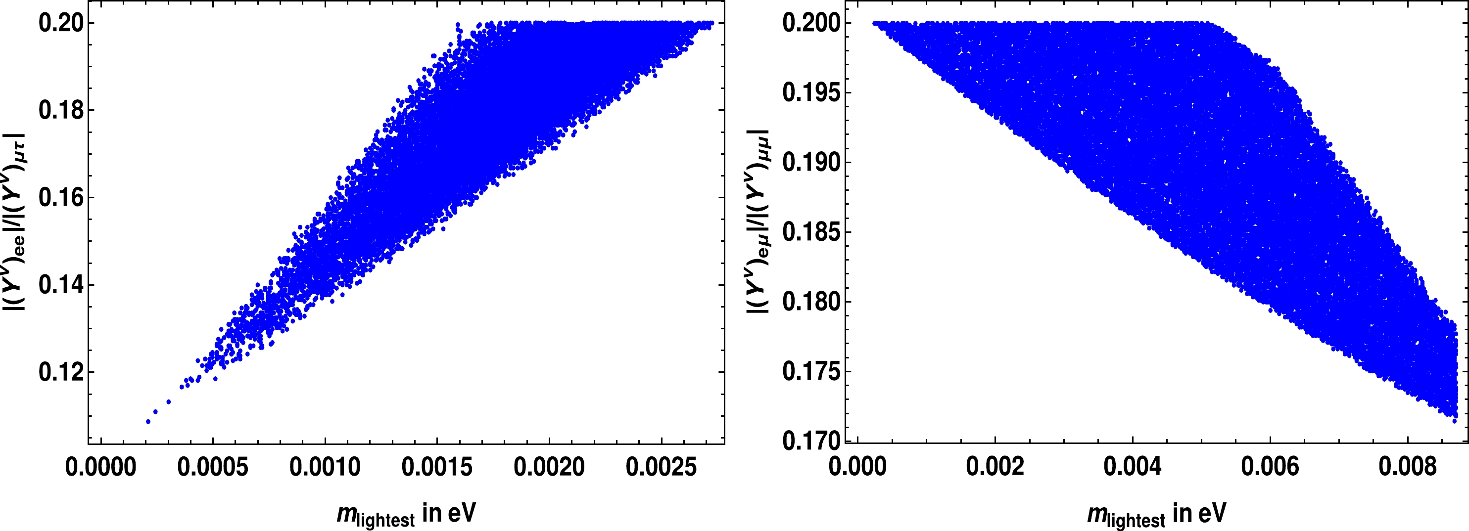
Figure 1. (color online) Ratios of the magnitude of Yukawa couplings versus the mass of lightest neutrino. The left- and right-hand side plots are for NO and IO, respectively. In both plots, we vary the neutrino oscillation observables over their allowed
$ 3\sigma $ ranges, which are given in Table 2. For other details, see the text.The conditions mentioned below Eq. (42), for both the NO and IO cases, cannot be achieved just with the
$C P$ symmetry. An additional mechanism should be proposed to satisfy these conditions. In an attempt towards this, we have proposed one mechanism to achieve condition (i) for the case of NO, where the necessary suppression in the Yukawa couplings is explained through non-renormalizable terms within the framework of$C P$ symmetry. This mechanism is presented in the Appendix. In this work, we do not have a mechanism to achieve condition (i) for the case of IO and to achieve condition (ii) for both NO and IO. These problems would be investigated in future works. As already described, with the generalized$C P$ transformations and$ \mu-\tau $ symmetry,$ \theta_{23} $ and$ \delta_{CP} $ will be maximal. However, in future neutrino oscillation experiments,$ \theta_{23} $ and$ \delta_{CP} $ may be found to be away from their maximal values. In such a case, one needs to device a mechanism for the breaking of$ \mu-\tau $ reflection symmetry in order to explain the non-maximal values for the above mentioned observables. However, these topics are outside the scope of the present study. -
In our proposed model for lepton mixing, three Higgs doublets exist. Since they can also give masses to quarks, it is interesting to check whether quark mixing can also be explained with
$C P$ and other symmetries of our model. As already described in Sec. I, since there is a hierarchy among quark masses, the mixing pattern for quarks can be explained if their Yukawa couplings are hierarchically suppressed. Babu and Nandi have proposed one model [27] for explaining quark mixing through hierarchically suppressed Yukawa couplings. Later, this model has been modified in Ref. [28], where the suppression in Yukawa couplings is explained with a singlet scalar field. We follow the work of Refs. [27, 28] to explain quark mixing in our framework. -
We denote the three families of quark doublets, up- and down-type singlets as
$ Q_{j{\rm L}} $ ,$ u_{j{\rm R}} $ and$ d_{j{\rm R}} $ , respectively. We propose a scalar field X, which is singlet under standard model gauge group. We assume all the quark fields to be singlets under the symmetry$ K\times Z_2\times Z_3 $ . The X field is singlet under$ K\times Z_3 $ but is odd under$ Z_2 $ . Both the quark and X fields transform under$C P$ symmetry as$ \begin{aligned}[b]& Q_{j{\rm L}}\to {\rm i}\gamma^0C\bar{Q}_{j{\rm L}}^T,\quad u_{j{\rm R}}\to {\rm i}\gamma^0C\bar{u}_{j{\rm R}}^T, \\& d_{j{\rm R}}\to {\rm i}\gamma^0C\bar{d}_{j{\rm R}}^T, \quad X\to X^*. \end{aligned} $

(43) Now, with the above mentioned transformations and fields, we consider the following effective Lagrangian for quark masses.
$ \begin{aligned}[b] {\cal L}_Y=&h^u_{33}\bar{Q}_{3{\rm L}}\tilde{\phi}_1u_{3{\rm R}} +\left(\frac{X}{M}\right)^2[h^d_{33}\bar{Q}_{3{\rm L}}\phi_1 d_{3{\rm R}} \\&+h^u_{22}\bar{Q}_{2{\rm L}}\tilde{\phi}_1u_{2{\rm R}} +h^u_{23}\bar{Q}_{2{\rm L}}\tilde{\phi}_1u_{3{\rm R}} \\ & +h^u_{32}\bar{Q}_{3{\rm L}}\tilde{\phi}_1 u_{2{\rm R}}]+\left(\frac{X}{M}\right)^4[h^d_{22}\bar{Q}_{2{\rm L}}\phi_1 d_{2{\rm R}} \\&+h^d_{23}\bar{Q}_{2{\rm L}}\phi_1 d_{3{\rm R}}+h^d_{32}\bar{Q}_{3{\rm L}}\phi_1 d_{2{\rm R}} \\ &+h^u_{12}\bar{Q}_{1{\rm L}}\tilde{\phi}_1u_{2{\rm R}}+h^u_{21}\bar{Q}_{2{\rm L}}\tilde{\phi}_1u_{1{\rm R}}\\&+h^u_{13}\bar{Q}_{1{\rm L}}\tilde{\phi}_1u_{3{\rm R}}+ h^u_{31}\bar{Q}_{3{\rm L}}\tilde{\phi}_1u_{1{\rm R}}] \\ &+\left(\frac{X}{M}\right)^6[h^u_{11}\bar{Q}_{1{\rm L}}\tilde{\phi}_1u_{1{\rm R}} +h^d_{11}\bar{Q}_{1{\rm L}}\phi_1 d_{1{\rm R}}\\&+h^d_{12}\bar{Q}_{1{\rm L}}\phi_1 d_{2{\rm R}} +h^d_{13}\bar{Q}_{1{\rm L}}\phi_1 d_{3{\rm R}}] \\ &+\left(\frac{X}{M}\right)^9[h^d_{21}\bar{Q}_{2{\rm L}}\phi_1 u_{1{\rm R}}] +\left(\frac{X}{M}\right)^{10}[h^d_{31}\bar{Q}_{3{\rm L}}\phi_1 u_{1{\rm R}}]+{\rm h.c}. \end{aligned} $

(44) The above Lagrangian is valid below a mass scale of M. The non-renormalizable terms of this Lagrangian can be motivated by the UV completion of this model, which is presented in the next subsection. According to this UV completion, we propose a flavor symmetry
$ U(1)_{\rm F} $ and heavy vector-like quark (VLQ) fields above the scale M. After integrating the heavy fields in our model, below the scale M, the non-renormalizable terms of Eq. (44) can appear. Here we can see that M represents the mass scale of heavy VLQs. Since new particles can be probed at the LHC experiment if their masses are around 1 TeV, we take$ M\sim $ 1 TeV.Due to
$C P$ symmetry, the Yukawa couplings$ h^{u,d}_{jk} $ should be real in Eq. (44). After X acquires VEV, for$ \langle X\rangle<M $ , we can see that$ {X}/{M} $ gives suppression to the effective quark Yukawa couplings. Since the Yukawa couplings of Eq. (44) are real, we assume$ \langle X\rangle $ is complex, and this can be the source for$C P$ violation in the quark sector. In the Lagrangian of Eq. (44), only the doublet$ \phi_1 $ generates Yukawa couplings for quark fields. The other doublets$ \phi_{2,3} $ do not generate these Yukawa couplings due to the presence of$C P\times K$ symmetry.After electroweak symmetry breaking, using Eq. (44), the matrices for up- and down-type quarks can be written, respectively, as
$ \begin{aligned}[b]& M_u=\left(\begin{array}{ccc} h^u_{11}\epsilon^6 & h^u_{12}\epsilon^4 & h^u_{13}\epsilon^4 \\ h^u_{21}\epsilon^4 & h^u_{22}\epsilon^2 & h^u_{23}\epsilon^2 \\ h^u_{31}\epsilon^4 & h^u_{32}\epsilon^2 & h^u_{33} \end{array}\right)v_1,\\& M_d=\left(\begin{array}{ccc} h^d_{11}\epsilon^6 & h^d_{12}\epsilon^6 & h^d_{13}\epsilon^6 \\ h^d_{21}\epsilon^9 & h^d_{22}\epsilon^4 & h^d_{23}\epsilon^4 \\ h^d_{31}\epsilon^{10} & h^d_{32}\epsilon^4 & h^d_{33}\epsilon^2 \end{array}\right)v_1. \end{aligned} $

(45) Here,
$ \epsilon=\dfrac{\langle X\rangle}{M} $ . The form of$ M_{u,d} $ is similar to the corresponding matrices in Refs. [27, 28]. However, the only difference is that the elements 21 and 31 of$ M_d $ are generated at a higher order compared to those in Refs. [27, 28]. It is argued in Ref. [28] that the above mentioned elements do not affect quark masses and mixing if they are generated at higher order. Hence, after diagonalizing the above matrices, the masses and mixing angles for quarks, up to leading order in$ |\epsilon| $ , are given by$ \begin{aligned}[b] &(m_t,m_c,m_u)\approx(|h^u_{33}|,|h^u_{22}||\epsilon|^2, |h^u_{11}-h^u_{12}h^u_{21}/h^u_{22}||\epsilon|^6)v_1, \\ &(m_b,m_s,m_d)\approx(|h^d_{33}||\epsilon|^2, |h^d_{22}||\epsilon|^4,|h^d_{11}||\epsilon|^6)v_1, \\ &|V_{us}|\approx\left|\frac{h^d_{12}}{h^d_{22}}- \frac{h^u_{12}}{h^u_{22}}\right||\epsilon|^2, \\ &|V_{cb}|\approx\left|\frac{h^d_{23}}{h^d_{33}}- \frac{h^u_{23}}{h^u_{33}}\right||\epsilon|^2, \\ &|V_{ub}|\approx\left|\frac{h^d_{13}}{h^d_{33}}- \frac{h^u_{12}h^d_{23}}{h^u_{22}h^d_{33}}- \frac{h^u_{13}}{h^u_{33}}\right||\epsilon|^4, \\ &{\rm arg}(V_{ub})\approx4{\rm arg}(\epsilon). \end{aligned} $

(46) Due to three Higgs doublets in our model, we have
$ |v_1|^2+|v_2|^2+|v_3|^2 \approx(174\; {\rm GeV})^2 $ . To satisfy this, we take$ v_1,v\sim174/\sqrt{2} $ GeV. With this value for$ v_1 $ , we fit the expressions of Eq. (46) to the following best fit values [18].$ \begin{aligned}[b] &(m_t,m_c,m_u)=(172.76,1.27,2.16\times10^{-3})\; {\rm GeV}, \\ &(m_b,m_s,m_d)=(4.18\times10^3,93,4.67)\; {\rm MeV}, \end{aligned} $

$ \begin{aligned}[b] &(|V_{us}|,|V_{cb}|,|V_{ub}|)=(0.2245,0.041,0.00382), \\ &{\rm arg}(V_{ub})=-1.196 \end{aligned} $

(47) After the abovementioned fitting, we give a sample set of numerical values with
$ |\epsilon|=1/5.5 $ as follows.$ \begin{aligned}[b] &(|h^u_{33}|,|h^u_{22}|, |h^u_{11}-h^u_{12}h^u_{21}/h^u_{22}|) \approx(1.4,0.31,0.49), \\ &(|h^d_{33}|,|h^d_{22}|,|h^d_{11}|)\approx (1.03,0.69,1.05), \\ &(h^d_{12},h^u_{12},h^d_{23},h^u_{23}, h^d_{13},h^u_{13})\\\approx&(1.49,-1.45,0.69,-0.8,1.12,1.0), \\ &{\rm arg}(\epsilon)\approx-0.3. \end{aligned} $

(48) From the numerical values given above, we can see that the magnitudes of all Yukawa couplings are less than about 1.5. We have considered numerical values with
$ |\epsilon|=1/6 $ . However, in this case, some of the Yukawa couplings can become larger than 2.0. Hence, with$ |\epsilon|=1/5.5 $ and$ {\cal O}(1) $ Yukawa couplings, we can explain the quark masses and mixing pattern in our model. Since we expect new physics to appear around 1 TeV, we can take the cut-off scale of Eq. (44) to be$ M\sim $ 1 TeV. Now, for$ |\epsilon|=1/5.5 $ , we get$ |\langle X\rangle|\sim $ 181 GeV. -
Here, we present the UV completion for our model in order to explain the origin of non-renormalizable terms of Eq. (44). To achieve this UV completion, we follow the works of Refs. [28, 38]. The idea of this UV completion is to explain non-renormalizable terms following from a theory which is renormalizable at a high scale. Hence, we assume our model is renormalizable at and above the scale M and propose a flavor symmetry
$ U(1)_{\rm F} $ , which is exactly above M. To generate non-renormalizable terms below M, we propose additional fields like flavons and VLQs, which transform under$ U(1)_{\rm F} $ . The standard model quarks are charged under the$ U(1)_{\rm F} $ symmetry. However, the Higgs doublets and X field are singlets under$ U(1)_{\rm F} $ . The$ U(1)_{\rm F} $ symmetry is spontaneously broken when the flavons acquire VEVs around M, which is also the mass scale of VLQs. Here, we can see that our model should respect the symmetry$C P\times K\times Z_2\times Z_3\times U(1)_{\rm F}$ above the scale M. However, below M, after integrating the heavy VLQs and flavon fields, our model should generate non-renormalizable terms of Eq. (44), which respect the symmetry$C P\times K\times Z_2\times Z_3$ .Under the
$ U(1)_{\rm F} $ , we denote the charges for$ Q_{j{\rm L}} $ ,$ u_{j{\rm R}} $ and$ d_{j{\rm R}} $ as$ q_{jf} $ ,$ u_{jf} $ and$ d_{jf} $ , respectively. We propose only two flavon fields,$ F_1 $ and$ F_2 $ , whose charges under$ U(1)_{\rm F} $ are$ f_1 $ and$ f_2 $ , respectively. Flavons are charged under$C P$ symmetry but are otherwise singlets under$ K\times Z_2\times Z_3 $ . Under the$C P$ symmetry, flavons transform like the X field of our model. Now, to generate non-renormalizable terms for up-type quarks in Eq. (44), we introduce VLQs$ K_{j{\rm L}} $ and$ K_{j{\rm R}} $ , which are color triplets and their hypercharges are same as those of right-handed singlet up-quarks. Analogous to$ K_{j{\rm L}} $ and$ K_{j{\rm R}} $ , we introduce$ G_{j{\rm L}} $ and$ G_{j{\rm R}} $ , which generate non-renormalizable terms for down-type quarks. The above VLQs are singlets under$S U(2)$ symmetry of the standard model and$ K\times Z_3 $ . These fields are charged under$ Z_2 $ symmetry. Under the$C P$ symmetry, they transform like the quark fields.After describing the field content and their charge assignments in the UV completion of our model, we further explain the generation of non-renormalizable terms of Eq. (44). The
$ h^u_{33} $ term in Eq. (44) is renormalizable, which can be generated in our model by taking$ q_{3f}=u_{3f} $ . To generate the$ h^u_{32} $ term in Eq. (44), we consider the below invariant terms in the UV completion.$ \begin{aligned}[b] \mathcal{L}^u_{32}=&\bar{Q}_{3{\rm L}}\tilde{\phi}_1 K_{1{\rm R}}+ F_1^*\bar{K}_{1{\rm R}}K_{1{\rm L}}+ X \bar{K}_{1{\rm L}}K_{2{\rm R}}\\& + F_2 \bar{K}_{2{\rm R}}K_{2{\rm L}}+ X \bar{K}_{2{\rm L}}u_{2{\rm R}}+{\rm h.c}.. \end{aligned} $

(49) Since the terms in the above equation are invariant under
$C P$ symmetry, the dimensionless Yukawa couplings should be real; these are$ {\cal O}(1) $ , which we have not written explicitly here. The$ U(1)_{\rm F} $ charges for$ K_{j{\rm L}},K_{j{\rm R}} $ can be fixed in terms of corresponding charges of quarks and flavons in such a way that the above equation is invariant under$ U(1)_{\rm F} $ . Similarly, the$ Z_2 $ charges for these VLQs can be assigned such that the above equation is invariant under$ Z_2 $ . The$ U(1)_{\rm F}\times Z_2 $ charges for VLQs of K-type are given in Eq. (57). When the flavons acquire VEVs, the VLQs in Eq. (49) acquire masses of the order of M. After integrating these heavy VLQs, terms in Eq. (49) generate the$ h^u_{32} $ term of Eq. (44).By introducing more VLQs of K-type, the process described in the previous paragraph can be applied to generate other non-renormalizable terms of Eq. (44). Below we show the invariant Lagrangians of the form
$ {\cal L}^u_{ij} $ , which generate the$ h^u_{ij} $ term of Eq. (44), after integrating the heavy VLQs and flavons. The$ U(1)_{\rm F}\times Z_2 $ charges for the VLQs in these Lagrangians can be seen in Eq. (57).$ \begin{aligned}[b] \mathcal{L}^u_{31}=& \bar{Q}_{3{\rm L}}\tilde{\phi}_1 K_{1{\rm R}}+ F_1^*\bar{K}_{1{\rm R}}K_{1{\rm L}}+ X \bar{K}_{1{\rm L}}K_{2{\rm R}}+ F_2 \bar{K}_{2{\rm R}}K_{2{\rm L}}+ X \bar{K}_{2{\rm L}}K_{3{\rm R}}+ F_2 \bar{K}_{3{\rm R}}K_{3{\rm L}} + X \bar{K}_{3{\rm L}}K_{4{\rm R}}+ M \bar{K}_{4{\rm R}}K_{4{\rm L}}\\ &+X\bar{K}_{4{\rm L}}u_{1{\rm R}}+{\rm h.c}.. \end{aligned} $ 
(50) $ \mathcal{L}^u_{23}= \bar{Q}_{2{\rm L}}\tilde{\phi}_1K_{5{\rm R}}+M\bar{K}_{5{\rm R}}K_{5{\rm L}}+X \bar{K}_{5{\rm L}}K_{6{\rm R}}+ F_1 \bar{K}_{6{\rm R}}K_{6{\rm L}}+X \bar{K}_{6{\rm L}}u_{3{\rm R}}+{\rm h.c}. $

(51) $ \mathcal{L}^u_{22}= \bar{Q}_{2{\rm L}}\tilde{\phi}_1K_{5{\rm R}}+M\bar{K}_{5{\rm R}}K_{5{\rm L}}+ X\bar{K}_{5{\rm L}}K_{7{\rm R}}+F_2 \bar{K}_{7{\rm R}}K_{7{\rm L}}+X\bar{K}_{7{\rm L}}u_{2{\rm R}}+{\rm h.c}. $

(52) $ \begin{aligned}[b] \mathcal{L}^u_{21}=&\bar{Q}_{2L}\tilde{\phi}_1K_{5{\rm R}}+M\bar{K}_{5{\rm R}}K_{5{\rm L}}+X\bar{K}_{5{\rm L}}K_{7{\rm R}}+F_2 \bar{K}_{7{\rm R}}K_{7{\rm L}}+X \bar{K}_{7{\rm L}}K_{8{\rm R}}+M\bar{K}_{8{\rm R}}K_{8{\rm L}}+ +X\bar{K}_{8{\rm L}}K_{9{\rm R}}+F_2\bar{K}_{9{\rm R}}K_{9{\rm L}}\\ &+X\bar{K}_{9{\rm L}}u_{1{\rm R}}+{\rm h.c}. \end{aligned} $

(53) $ \begin{aligned}[b] \mathcal{L}^u_{11}=& \bar{Q}_{1{\rm L}}\tilde{\phi}_1K_{10{\rm R}}+F_2 \bar{K}_{10{\rm R}}K_{10{\rm L}}+X\bar{K}_{10{\rm L}}K_{11{\rm R}}+F_2 \bar{K}_{11{\rm R}}K_{11{\rm L}} +X\bar{K}_{11{\rm L}}K_{12{\rm R}} F_2\bar{K}_{12{\rm R}}K_{12{\rm L}}+X\bar{K}_{12{\rm L}}K_{13{\rm R}}\\ &+F_2 \bar{K}_{13{\rm R}}K_{13{\rm L}}+X\bar{K}_{13{\rm L}}K_{14{\rm R}}+F_2 \bar{K}_{14{\rm R}}K_{14{\rm L}} + X\bar{K}_{14{\rm L}}K_{15{\rm R}}+M\bar{K}_{15{\rm R}}K_{15{\rm L}}+X\bar{K}_{15{\rm L}}u_{1{\rm R}}+{\rm h.c}.. \end{aligned} $

(54) $ \begin{aligned}[b] \mathcal{L}^u_{12}=& \bar{Q}_{1{\rm L}}\tilde{\phi}_1K_{10{\rm R}}+F_2 \bar{K}_{10{\rm R}}K_{10{\rm L}}+X\bar{K}_{10{\rm L}}K_{11{\rm R}}+F_2 \bar{K}_{11{\rm R}}K_{11{\rm L}}+X\bar{K}_{11{\rm L}}K_{12{\rm R}} +F_2\bar{K}_{12{\rm R}}K_{12{\rm L}}+X\bar{K}_{12{\rm L}}K_{13{\rm R}}\\ &+F_2 \bar{K}_{13{\rm R}}K_{13{\rm L}}+X\bar{K}_{13{\rm L}}u_{2{\rm R}}+{\rm h.c}.. \end{aligned} $

(55) $ \begin{aligned}[b] \mathcal{L}^u_{13}=& \bar{Q}_{1{\rm L}}\tilde{\phi}_1K_{10{\rm R}}+F_2 \bar{K}_{10{\rm R}}K_{10{\rm L}}+X\bar{K}_{10{\rm L}}K_{11{\rm R}}+F_2 \bar{K}_{11{\rm R}}K_{11{\rm L}}+X\bar{K}_{11{\rm L}}K_{12{\rm R}} +F_2\bar{K}_{12{\rm R}}K_{12{\rm L}}\\ &+X\bar{K}_{12{\rm L}}K_{16{\rm R}}+F_1 \bar{K}_{16{\rm R}}K_{16{\rm L}}+X\bar{K}_{16{\rm L}}u_{3{\rm R}}+{\rm h.c}.. \end{aligned} $

(56) $ \begin{aligned}[b] U(1)_{\rm F}\;:\;& K_{1{\rm R}}\rightarrow q_{3f},\quad K_{1{\rm L}}, K_{2{\rm R}}\rightarrow q_{3f}+f_1,\quad K_{2{\rm L}}, K_{3{\rm R}}\rightarrow q_{3f}+f_1-f_2, \quad K_{3{\rm L}},K_{4{\rm L}}, K_{4{\rm R}}\rightarrow q_{3f}+f_1-2f_2,\\ & K_{5{\rm R}}, K_{5{\rm L}},K_{6{\rm R}},K_{7{\rm R}}\rightarrow q_{2f} \quad K_{7{\rm L}},K_{8{\rm R}},K_{8{\rm L}},K_{9{\rm R}}\rightarrow q_{2f}-f_2,\quad K_{6{\rm L}}\rightarrow q_{2f}-f_1,\quad K_{9{\rm L}}\rightarrow q_{2f}-2 f_2, \\ & K_{10{\rm R}}\rightarrow q_{1f},\quad K_{10{\rm L}},K_{11{\rm R}}\rightarrow q_{1f}-f_2,\quad K_{11{\rm L}},K_{12{\rm R}}\rightarrow q_{1f}-2 f_2, \quad K_{12{\rm L}},K_{13{\rm R}},K_{16{\rm R}}\rightarrow q_{1f}-3 f_2, \\ & K_{13{\rm L}},K_{14{\rm R}}\rightarrow q_{1f}-4 f_2, \quad K_{14{\rm L}},K_{15{\rm R}},K_{15{\rm L}}\rightarrow q_{1f}-5 f_2,\quad K_{16{\rm L}},u_{3{\rm R}}\rightarrow q_{1f}-3 f_2-f_1. \\ Z_2 \;:\;& K_{1{\rm L}}, K_{1{\rm R}}, K_{3{\rm L}}, K_{3{\rm R}},K_{5{\rm L}}, K_{5{\rm R}},K_{8{\rm L}},K_{8{\rm R}}, K_{10{\rm L}},K_{10{\rm R}},K_{12{\rm L}},K_{12{\rm R}},K_{14{\rm L}},K_{14{\rm R}}, \rightarrow \rm{even},\\ & K_{2{\rm L}}, K_{2{\rm R}}, K_{4{\rm L}}, K_{4{\rm R}},K_{6{\rm L}},K_{6{\rm R}},K_{7{\rm L}}, K_{7{\rm R}},K_{9{\rm L}},K_{9{\rm R}},K_{11{\rm L}},K_{11{\rm R}}, K_{13{\rm L}},K_{13{\rm R}},K_{15{\rm R}},K_{15{\rm L}},K_{16{\rm L}},K_{16{\rm R}}\rightarrow \rm{odd}. \end{aligned} $

(57) Since the Lagragians of Eqs. (49) –(56) are invariant under
$ U(1)_{\rm F} $ , we get relations among the$ U(1)_{\rm F} $ charges of quarks and flavons. These relations can be consistently solved. Taking$ q_{3f} $ ,$ f_1 $ , and$ f_2 $ as independent variables, the above mentioned relations can be expressed as$ \begin{aligned}[b] &q_{2f}=q_{3f}+f_1,\quad q_{1f}=q_{3f}+f_1+3f_2,\quad u_{3f}=q_{3f},\quad \\ & u_{2f}=q_{3f}+f_1-f_2,\quad u_{1f}=q_{3f}+f_1-2f_2. \end{aligned} $

(58) The procedure described above has been applied in order to generate non-renormalizable terms for down-type quarks of Eq. (44). In this case, we introduce VLQs
$ G_{i{\rm R}},G_{i{\rm L}} $ , where$ i=1,\cdots,30 $ . Below, we give invariant Lagrangians in the form of$ {\cal L}^d_{ij} $ , which generate the$ h^d_{ij} $ term in Eq. (44), after integrating the heavy VLQs and flavons. Since these Lagrangians are invariant under the$ U(1)_{\rm F}\times Z_2 $ , the charges of VLQs under this symmetry are fixed in terms of corresponding charges of quarks and flavons. These charges are given in Eq. (68).$ \mathcal{L}^d_{33}= \bar{Q}_{3{\rm L}}\phi_1 G_{1{\rm R}}+ F_1 \bar{G}_{1{\rm R}}G_{1{\rm L}}+X \bar{G}_{1{\rm L}}G_{2{\rm R}}+ F_1 \bar{G}_{2{\rm R}}G_{2{\rm L}}+ X \bar{G}_{2{\rm L}}d_{3{\rm R}}+{\rm h.c}.. $ 
(59) $ \begin{aligned}[b] \mathcal{L}^d_{32}=& \bar{Q}_{3{\rm L}}\phi_1 G_{1{\rm R}}+ F_1 \bar{G}_{1{\rm R}}G_{1{\rm L}}+ X \bar{G}_{1{\rm L}}G_{2{\rm R}}+ F_1 \bar{G}_{2{\rm R}}G_{2{\rm L}}+ X \bar{G}_{2{\rm L}}G_{3{\rm R}} + M \bar{G}_{3{\rm R}}G_{3{\rm L}} + X \bar{G}_{3{\rm L}}G_{4{\rm R}}\\&+ F_2^*\bar{G}_{4{\rm R}}G_{4{\rm L}}+ X \bar{G}_{4{\rm L}}d_{2{\rm R}}+ {\rm h.c}.. \end{aligned} $

(60) $ \begin{aligned}[b] \mathcal{L}^d_{23} = & \bar{Q}_{2{\rm L}}\phi_1 G_{5{\rm R}}+ F_1 \bar{G}_{5{\rm R}}G_{5{\rm L}}+X\bar{G}_{5{\rm L}}G_{6{\rm R}}+F_1 \bar{G}_{6{\rm R}}G_{6{\rm L}}+X \bar{G}_{6{\rm L}}G_{7{\rm R}} +F_1 \bar{G}_{7{\rm R}}G_{7{\rm L}}+ X \bar{G}_{7{\rm L}}G_{8{\rm R}}\\&+M \bar{G}_{8{\rm R}}G_{8{\rm L}}+\bar{G}_{8{\rm L}}d_{3{\rm R}}+{\rm h.c}.. \end{aligned} $

(61) $ \begin{aligned}[b] \mathcal{L}^d_{22}=& \bar{Q}_{2{\rm L}}\phi_1 G_{5{\rm R}}+ F_1 \bar{G}_{5{\rm R}}G_{5{\rm L}}+X\bar{G}_{5{\rm L}}G_{6{\rm R}}+F_1 \bar{G}_{6{\rm R}}G_{6{\rm L}}+X \bar{G}_{6{\rm L}}G_{7{\rm R}} +F_1 \bar{G}_{7{\rm R}}G_{7{\rm L}}+X\bar{G}_{7{\rm L}}G_{9{\rm R}}\\&+F_2^* \bar{G}_{9{\rm R}}G_{9{\rm L}}+X\bar{G}_{9{\rm L}}d_{2{\rm R}}+{\rm h.c}.. \end{aligned} $

(62) $ \begin{aligned}[b] \mathcal{L}^d_{13}=& \bar{Q}_{1{\rm L}}\phi_1 G_{10{\rm R}}+F_1 \bar{G}_{10{\rm R}}G_{10{\rm L}}+X\bar{G}_{10{\rm L}}G_{11{\rm R}}+ +F_1 \bar{G}_{11{\rm R}}G_{11{\rm L}}+X\bar{G}_{11{\rm L}}G_{12{\rm R}} +F_1 \bar{G}_{12{\rm R}}G_{12{\rm L}}+X \bar{G}_{12{\rm L}}G_{13{\rm R}}\\ &+F_2 \bar{G}_{13{\rm R}}G_{13{\rm L}}+X \bar{G}_{13{\rm L}}G_{14{\rm R}}+F_2 \bar{G}_{14{\rm R}}G_{14{\rm L}}+X \bar{G}_{14{\rm L}}G_{15{\rm R}}+F_2 \bar{G}_{15{\rm R}}G_{15{\rm L}}+X\bar{G}_{15{\rm L}}d_{3{\rm R}}+{\rm h.c}.. \end{aligned} $

(63) $ \begin{aligned}[b] \mathcal{L}^d_{12}=& \bar{Q}_{1{\rm L}}\phi_1 G_{10{\rm R}}+F_1 \bar{G}_{10{\rm R}}G_{10{\rm L}}+X\bar{G}_{10{\rm L}}G_{11{\rm R}}+F_1 \bar{G}_{11{\rm R}}G_{11{\rm L}}+X\bar{G}_{11{\rm L}}G_{12{\rm R}} +F_1 \bar{G}_{12{\rm R}}G_{12{\rm L}}+X \bar{G}_{12{\rm L}}G_{13{\rm R}}\\ &+F_2 \bar{G}_{13{\rm R}}G_{13{\rm L}}+X \bar{G}_{13{\rm L}}G_{14{\rm R}}+F_2 \bar{G}_{14{\rm R}}G_{14{\rm L}} X \bar{G}_{14{\rm L}}G_{16{\rm R}}+M \bar{G}_{16{\rm R}}G_{16{\rm L}}+X\bar{G}_{16{\rm L}}d_{2{\rm R}}+{\rm h.c}.. \end{aligned} $

(64) $ \begin{aligned}[b] \mathcal{L}^d_{11}=&\bar{Q}_{1{\rm L}}\phi_1 G_{10{\rm R}}+F_1 \bar{G}_{10{\rm R}}G_{10{\rm L}}+X\bar{G}_{10{\rm L}}G_{11{\rm R}} +F_1 \bar{G}_{11{\rm R}}G_{11{\rm L}}+X\bar{G}_{11{\rm L}}G_{12{\rm R}} +F_1 \bar{G}_{12{\rm R}}G_{12{\rm L}}+X\bar{G}_{12{\rm L}}G_{17{\rm R}}\\ &+F_1 \bar{G}_{17{\rm R}}G_{17{\rm L}}+X\bar{G}_{17{\rm L}}G_{18{\rm R}} +F_1\bar{G}_{18{\rm R}}G_{18{\rm L}} +X\bar{G}_{18{\rm L}}G_{19{\rm R}}+F_2^* \bar{G}_{19{\rm R}}G_{19{\rm L}}+X\bar{G}_{19{\rm L}}d_{1{\rm R}}+{\rm h.c}.. \end{aligned} $

(65) $ \begin{aligned}[b] \mathcal{L}^d_{21}=& \bar{Q}_{2L}\phi_1 M_{5R}+ F_1 \bar{G}_{5R}G_{5L}+X\bar{G}_{5L}G_{6R}+F_1 \bar{G}_{6R}G_{6L}+X \bar{G}_{6L}G_{7R}+F_1 \bar{G}_{7R}G_{7L} +X\bar{G}_{7L}G_{9R}+F_2^* \bar{G}_{9R}G_{9L} \\ &+ X\bar{G}_{9L}G_{20R} + F_2^*\bar{G}_{20R}G_{20L} +X\bar{G}_{20L}G_{21R}+F_2^* \bar{G}_{21R}G_{21L} + X\bar{G}_{21L}G_{22R}+ F_2^* \bar{G}_{22R}G_{22L}\\ &+ X\bar{G}_{22L}G_{23R} +F_1 \bar{G}_{23R}G_{23L} + X \bar{G}_{23L}G_{24R} + F_1\bar{G}_{24R}G_{24L} + X \bar{G}_{24L}d_{1R}+h.c.. \end{aligned} $

(66) $ \begin{aligned}[b] \mathcal{L}^d_{31}=& \bar{Q}_{3{\rm L}}\phi_1 G_{1{\rm R}}+ F_1 \bar{G}_{1{\rm R}}G_{1{\rm L}}+ X \bar{G}_{1{\rm L}}G_{2{\rm R}}+ F_1 \bar{G}_{2{\rm R}}G_{2{\rm L}}+ X\bar{G}_{2{\rm L}}G_{25{\rm R}} +F_1\bar{G}_{25{\rm R}}G_{25{\rm L}} + X\bar{G}_{25{\rm L}}G_{26{\rm R}} + F_1 \bar{G}_{26{\rm R}}G_{26{\rm L}} \\&+ X\bar{G}_{26{\rm L}}G_{27{\rm R}} + F_2^*\bar{G}_{27{\rm R}}G_{27{\rm L}}+X\bar{G}_{27{\rm L}}G_{28{\rm R}}+F_2^* \bar{G}_{28{\rm R}}G_{28{\rm L}} + X\bar{G}_{28{\rm L}}G_{29{\rm R}} \\&+ F_2^*\bar{G}_{29{\rm R}}G_{29{\rm L}} +X\bar{G}_{29{\rm L}}G_{30{\rm R}} +F_2^*\bar{G}_{30{\rm R}}G_{30{\rm L}} + X \bar{G}_{30L}d_{1{\rm R}}+{\rm h.c}.. \end{aligned} $

(67) $ \begin{aligned}[b] U(1)_F \;\;:\;\;& G_{1{\rm R}}\rightarrow q_{3f},\quad G_{1{\rm L}},G_{2{\rm R}}\rightarrow q_{3f}-f_1\quad G_{2{\rm L}},G_{3{\rm R}},G_{3{\rm L}},G_{4{\rm R}},G_{25{\rm R}}\rightarrow q_{3f}-2f_1, \\ & G_{4{\rm L}}\rightarrow q_{3f}-2f_1+f_2,\quad G_{5{\rm R}}\rightarrow q_{2f},\quad G_{5{\rm L}},G_{6{\rm R}}\rightarrow q_{2f}-f_1, \\ & G_{6{\rm L}},G_{7{\rm R}}\rightarrow q_{2f}-2f_1,\quad G_{7{\rm L}},G_{8{\rm R}},G_{8{\rm L}},G_{9{\rm R}}\rightarrow q_{2f}-3 f_1 \\ & G_{9{\rm L}},G_{20{\rm R}}\rightarrow q_{2f}-3 f_1+f_2,\quad G_{10{\rm R}}\rightarrow q_{1f},\quad G_{10{\rm L}},G_{11{\rm R}}\rightarrow q_{1f}-f_1, \\ & G_{11{\rm L}},G_{12{\rm R}}\rightarrow q_{1f}-2 f_1,\quad G_{12{\rm L}},G_{13{\rm R}},G_{17{\rm R}}\rightarrow q_{1f}-3 f_1, \\ &G_{13{\rm L}},G_{14{\rm R}}\rightarrow q_{1f}-3 f_1-f_3,\quad G_{14{\rm L}},G_{15{\rm R}},G_{16{\rm L}},G_{16{\rm R}}\rightarrow q_{1f}-3 f_1-2 f_2 \end{aligned} $

$ \begin{aligned}[b] & G_{15{\rm L}}\rightarrow q_{1f}-3 f_1-3f_3,\quad G_{17{\rm L}},G_{18{\rm R}}\rightarrow q_{1f}-4 f_1,\quad G_{18{\rm L}},G_{19{\rm R}}\rightarrow q_{1f}-5 f_1, \\ & G_{19{\rm L}}\rightarrow q_{1f}-5 f_1-f_2,\quad G_{20{\rm L}},G_{21{\rm R}}\rightarrow q_{2f}-3 f_1+2 f_2, \\ & G_{21{\rm L}},G_{22{\rm R}}\rightarrow q_{2f}-3f_1+3 f_2,\quad G_{22{\rm L}},G_{23{\rm R}}\rightarrow q_{2f}-3 f_1+4 f_2, \\ & G_{23{\rm L}},G_{24{\rm R}}\rightarrow q_{2f}–4 f_1+4 f_2,\quad G_{24{\rm L}}\rightarrow q_{2f}-5 f_1+4 f_2, \\ & G_{25{\rm L}},G_{26{\rm R}}\rightarrow q_{3f}-3 f_1,\quad G_{26{\rm L}},G_{27{\rm R}{\rm R}}\rightarrow q_{3f}-4 f_1,\quad G_{27{\rm L}}, G_{28{\rm R}}\rightarrow q_{3f}-4 f_1+f_2, \\ & G_{28{\rm L}},G_{29{\rm R}}\rightarrow q_{3f}-4 f_1+2 f_2,\quad G_{29{\rm L}},G_{30{\rm R}}\rightarrow q_{3f}-4 f_1+3 f_2, \\ & g_{30{\rm L}}\rightarrow q_{3f}-4 f_1+4 f_2. \\ Z_2 \;\;:\;\;& G_{1{\rm L}},G_{1{\rm R}}, G_{3{\rm L}}, G_{3{\rm R}}, G_{5{\rm L}}, G_{5{\rm R}}, G_{7{\rm L}}, G_{7{\rm R}}, G_{10{\rm L}}, G_{10{\rm R}},G_{12{\rm L}}, G_{12{\rm R}}, G_{14{\rm L}}, G_{14{\rm R}}, G_{18{\rm L}}, \\ &G_{18{\rm R}}, G_{20{\rm L}}, G_{20{\rm R}}, G_{22{\rm L}}, G_{22{\rm R}}, G_{24{\rm L}}, G_{24{\rm R}}, G_{25{\rm L}}, G_{25{\rm R}}, G_{27{\rm L}}, G_{27{\rm R}}, G_{29{\rm L}}, G_{29{\rm R}} \rightarrow \rm{even}. \\ & G_{2{\rm L}},G_{2{\rm R}}, G_{4{\rm L}}, G_{4{\rm R}}, G_{6{\rm L}}, G_{6{\rm R}}, G_{8{\rm L}}, G_{8{\rm R}}, G_{9{\rm L}}, G_{9{\rm R}}, G_{11{\rm L}}, G_{11R}, G_{13{\rm L}}, G_{13{\rm R}},G_{15{\rm L}}, \\ & G_{15{\rm R}}, G_{16{\rm L}}, G_{16{\rm R}}, G_{17{\rm L}}, G_{17{\rm R}}, G_{19{\rm L}}, G_{19{\rm R}}, G_{21{\rm L}}, G_{21{\rm R}}, G_{23{\rm L}}, G_{23{\rm R}}, G_{26{\rm L}}, G_{26{\rm R}}, \\ & G_{28{\rm L}}, G_{28{\rm R}}, G_{30{\rm L}}, G_{30{\rm R}} \rightarrow \rm{odd}. \end{aligned} $

(68) Since the Lagrangians in Eqs. (59)–(67) are invariant under
$ U(1)_{\rm F} $ , nine relations emerge among the$ U(1)_{\rm F} $ charges of quarks and flavons. These relations can be solved consistently along with Eq. (58). After doing this, the$ U(1)_{\rm F} $ charges of singlet down-type quarks can be expressed as$ \begin{equation} d_{3f}=q_{3f}-2f_1,\quad d_{2f}=q_{3f}-2f_1+f_2,\quad d_{1f}=q_{3f}-4f_1+4f_2. \end{equation} $

(69) In this section, we have described our model for the quark sector as well as the UV completion to it. As part of this whole construction, we introduce extra fields and symmetries into our model, which are summarized in Table 3.
Additional field Role X to generate hierarchy in quark masses and also $C P$ violation in quark sector

$ F_1,F_2 $ 

to generate masses for VLQs in the UV completion of our model $K_{i{\rm L}},K_{i{\rm R}}$ (

$ i=1,\cdots,16 $ )

to generate effective Yukawa couplings for up-type quarks from UV completion our model $G_{i{\rm L} },G_{i{\rm R} }$ (

$ i=1,\cdots,30 $ )

to generate effective Yukawa couplings for down-type quarks from UV completion our model Additional symmetry Role U(1)F to generate invariant terms in the UV completion of our model Table 3. Additional fields and symmetry, along with their roles, in the quark sector of our model.
-
In Sec. III, we have detailed the analysis of scalar potential for the model described in Sec. II. However, the model in Sec. II addresses problems related to the masses of leptons. Later, within the framework of that model, we have addressed the hierarchy in the masses of quark fields in Sec. V. Concurrently, we have introduced additional singlet scalar fields:
$ X,\;F_1,\;F_2 $ , which can give extra terms with the doublet and triplet Higgses in the scalar potential. These extra terms may change the results derived in Sec. III. For this purpose, in this section, we give the full scalar potential of our model. After minimizing the full scalar potential, we demonstrate that the above mentioned singlet scalar fields do not change the main conclusions of the analysis made in Sec. III. We recall the following main conclusions of Sec. III: (i) triplet Higgs acquire real VEV, (ii) VEVs of doublet Higgses$ \Phi_{2,3} $ explain the hierarchy between$ m_\mu $ and$ m_\tau $ .The full scalar potential of our model is
$ \begin{array}{*{20}{l}} V_{{\rm full}}=V_{\rm inv}+ V_{X,F_1,F_2}+V_{\not{K}}+V^\prime_{\not{K}}. \end{array} $

(70) Here,
$ V_{X,F_1,F_2} $ is the invariant scalar potential of our model, arising due to the singlet fields$ X,\;F_1,\;F_2 $ .$ V^\prime_{\not{K}} $ contains potential terms due to$ X,\;F_1,\;F_2 $ , which violate K-symmetry explicitly. Recall that the minimization of$ V_{\rm inv}+V_{\not{K}} $ has been discussed in Sec. III. First we find a minimum for$ V_{\rm inv}+V_{X,F_1,F_2} $ . Further, we study the shift in this minimum due to the presence of K-violating terms. In this regard, the minimization of$ V_{\rm inv} $ , after applying the$ Z_3 $ symmetry, has been studied in Sec. III.C. Here, we verify whether this minimization can be affected by$ V_{X,F_1,F_2} $ . The form for this potential is given below.$ \begin{aligned}[b]\\ V_{X,F_1,F_2}=&-m_X^2 (X^*X)-m_{F_1}^2(F_1^* F_1)-m_{F_2}^2(F_2^* F_2)+\lambda_X (X^*X)^2 +\lambda_{F_1}(F_1^* F_1)^2 +\lambda_{F_2}(F_2^* F_2)^2+ A(X^2+{X^*}^2)\\ &+B(X^4+{X^*}^4)+ \lambda_X^{\prime}(X^3X^{*}+{X^*}^3X) +\lambda_{F_1F_2}(F_1^* F_1)(F_2^* F_2) +\lambda_{F_1 X}(F_1^*F_1)(X^*X) +\lambda_{F_1 X}^{\prime}(F_1^*F_1)(X^2+{X^*}^2) \\ &+\lambda_{F_2 X}(F_2^*F_2)(X^*X)+\lambda_{F_2 X}^{\prime}(F_2^*F_2)(X^2+{X^*}^2) +\lambda_{\phi_1 X}(\phi_1^{\dagger}\phi_1)(X^*X) +\lambda_{\phi_1 X}^{\prime}(\phi_1^{\dagger}\phi_1)(X^2+{X^*}^2)\\ &+\lambda_{\phi_2 X}(\phi_2^{\dagger}\phi_2+\phi_3^{\dagger}\phi_3)(X^*X)+\lambda_{\phi_2 X}^{\prime}(\phi_2^{\dagger}\phi_2+\phi_3^{\dagger}\phi_3)(X^2+{X^*}^2)+\lambda_{\Delta X}\rm Tr(\Delta^{\dagger}\Delta)(X^*X) +\lambda_{\Delta X}^{\prime}{\rm Tr}(\Delta^{\dagger}\Delta)(X^2+{X^*}^2)\\ &+\lambda_{F_1\phi_1}(F_1^*F_1)(\phi_1^{\dagger}\phi_1)+\lambda_{F_2\phi_1}(F_2^*F_2)(\phi_1^{\dagger}\phi_1) +\lambda_{F_1\phi_2}(F_1^*F_1)(\phi_2^{\dagger}\phi_2+\phi_3^{\dagger}\phi_3)+\lambda_{F_2\phi_2}(F_2^*F_2)(\phi_2^{\dagger}\phi_2+\phi_3^{\dagger}\phi_3) \\ & +\lambda_{F_1\Delta}{\rm Tr}(\Delta^{\dagger}\Delta)(F_1^*F_1)+\lambda_{F_2\Delta}{\rm Tr}(\Delta^{\dagger}\Delta)(F_2^*F_2). \end{aligned} $ 
(71) In the above equation, all parameters are real due to hermiticity and
$C P$ symmetry.In Eq. (71),
$ F_1 $ and$ F_2 $ appear in the form of$ F_1^*F_1 $ and$ F_2^*F_2 $ , respectively. As a result, we can consider the VEVs of$ F_1 $ and$ F_2 $ to be real. Hence, we can parameterize the VEVs for$ X,F_1,F_2 $ as$ \begin{array}{*{20}{l}} \langle X \rangle =v_{X}{\rm e}^{{\rm i}\theta_{X}},\quad \langle F_1 \rangle =v_{f_1},\quad \langle F_2 \rangle =v_{f_2}. \end{array} $

(72) Here,
$ \theta_X $ is the phase in the VEV of X. After using the above VEVs and Eq. (17) in Eq. (71), we get$ \begin{aligned}[b] \langle V_{X,F_1,F_2}\rangle \ni& 2 v_X^2\Big[ A +\lambda_X^{\prime} v_X^2 +\lambda_{\phi_1 X}^{\prime}v_1^2+\lambda_{\phi_2 X}^{\prime}v^2+\lambda_{\Delta X}{v^{\prime}}^2\\&+\lambda_{F_1 X}^{\prime}v_{f_1}^2+ +\lambda_{F_2 X}^{\prime}v_{f_2}^2\Big]\cos2\theta_X +2 B v_X^4 \cos4\theta_{X}. \end{aligned} $

(73) In the above equation, we have not written constant terms which do not contain phases of the VEVs of the fields. It is possible to notice that
$ \theta_X $ do not mix with the phases in the VEVs of$ \phi_{2,3} $ and Δ. Hence, the minimization of$ \langle V_{\rm inv}\rangle $ , which is presented in Sec. III.C, is not affected due to$ \langle V_{X,F_1,F_2}\rangle $ . Consequently, Δ can acquire a real VEV, while Eq. (34) remains valid. From the minimization of$ \langle V_{X,F_1,F_2}\rangle $ with respect to$ \theta_X $ , we get$ \begin{aligned}[b] \cos2\theta_{X}=&-\frac{1}{4 B v_X^2}\Big[A+\lambda_X^{\prime}v_X^2+\lambda_{\phi_1 X}^{\prime}v_1^2+\lambda_{\phi_2 X}^{\prime}v^2\\ &+\lambda_{\Delta X}^{\prime}{v^{\prime}}^2+\lambda_{F_1 X}^{\prime}v_{f_1}^2+\lambda_{F_2 X}^{\prime}v_{f_2}^2\Big]. \end{aligned} $

(74) The above relation corresponds to the minimum for
$ \theta_X $ , provided the below condition is satisfied.$ \begin{aligned}[b] 16 B^2 v_X^4 >& \Big[A+\lambda_X^{\prime}v_X^2+\lambda_{\phi_1 X}^{\prime}v_1^2+\lambda_{\phi_2 X}^{\prime}v^2+\lambda_{\Delta X}^{\prime}{v^{\prime}}^2\\&+\lambda_{F_1 X}^{\prime}v_{f_1}^2+\lambda_{F_2 X}^{\prime}v_{f_2}^2\Big]^2 . \end{aligned} $

(75) Here we have shown that X can acquire complex VEV. This must be achieved to generate the
$ CP $ violation in the quark sector, which is discussed in Sec. V.After minimizing
$ \langle V_{\rm inv}\rangle+\langle V_{X,F_1,F_2}\rangle $ , we have shown that the minimum can be given by Eqs. (34) and (74). This minimum can be shifted by small amount due to K-violating terms. Terms in$ V_{\not{K}} $ are presented in Sec. III. Below we give the form for$ V_{\not{K}}^\prime $ .$ \begin{aligned}[b] V_{\not{K}}^{\prime}=& \delta\lambda_{\phi_2 X}(\phi_2^{\dagger}\phi_2)(X^*X)+\delta\lambda_{\phi_2 X}^{\prime}(\phi_3^{\dagger}\phi_3)(X^*X)+\delta\lambda_{\phi X}(\phi_2^{\dagger}\phi_2)(X^2+{X^*}^2) +\delta\lambda_{\phi X}^{\prime}(\phi_3^{\dagger}\phi_3)(X^2+{X^*}^2)\\ &+\delta \lambda_{\phi_2 F_1}(\phi_2^{\dagger}\phi_2)(F_1^{*}F_1)+\delta \lambda_{\phi_2 F_1}^{\prime}(\phi_3^{\dagger}\phi_3)(F_1^{*}F_1) +\delta \lambda_{\phi_2 F_2}(\phi_2^{\dagger}\phi_2)(F_2^{*}F_2)+\delta \lambda_{\phi_2 F_2}^{\prime}(\phi_3^{\dagger}\phi_3)(F_2^{*}F_2)\\&+{\rm i}\delta\lambda_{21}(\phi_2^{\dagger}\phi_3-\phi_3^{\dagger}\phi_2)(X^*X) +{\rm i}\delta\lambda_{22}(\phi_2^{\dagger}\phi_3-\phi_3^{\dagger}\phi_2)(X^2+{X^*}^2)+{\rm i}\delta\lambda_{23}(\phi_2^{\dagger}\phi_3-\phi_3^{\dagger}\phi_2)(F_1^*F_1) +{\rm i}\delta\lambda_{24}(\phi_2^{\dagger}\phi_3-\phi_3^{\dagger}\phi_2)(F_2^*F_2). \end{aligned} $ 
(76) All parameters in the above equation are real due to either
$C P$ symmetry or hermiticity of the potential. These parameters should be small compared to those in$ V_{\rm inv}+V_{X,F_1,F_2} $ , since the above potential violates K symmetry by a small amount. We can see that the VEVs of$ X,F_1,F_2 $ in$ V_{\not{K}}^\prime $ can give additional contribution to$ f_0 $ and$ f_\zeta $ in Eq. (36). Since the parameters of$ V_{\not{K}}^\prime $ are small, we can notice that the contribution due to$ X,F_1,F_2 $ can be of the same order as the terms already obtained for$ f_0 $ and$ f_\zeta $ in Eq. (36). As a result, the hierarchy in$ m_\mu $ and$ m_\tau $ can be explained in our framework. -
In Secs. III and VI we have analyzed the minimum of the scalar potential of our model. One needs to study whether this minimum corresponds to a global or local minimum. Following the studies made in Refs. [39, 40], we expect some additional conditions to be imposed on the parameters of our model in order for the minimum of the potential in this work to be global. Nonetheless, we shall work on the vacuum stability of our scalar potential in future studies.
The scalar fields, which are proposed in our model, are: three Higgs doublets, one Higgs triplet and three singlet scalar fields. We can choose the
$ U(1)_{\rm F} $ symmetry of our model to be gauged. As a result, after electroweak symmetry breaking, the following fields remain in the theory: one doubly charged scalar, three singly charged scalars, seven neutral scalars, and five pseudo scalars. In case I, which is described in Sec. III, the scalar fields belonging to the triplet Higgs can have masses around$ 10^{12} $ GeV. Otherwise, we can choose the parameters in the scalar potential of our model in such a way that all the scalar fields can have masses less than or about 1 TeV. In the case where the masses for the scalar fields are less than 1 TeV, one can study the collider phenomenology. For this study, one needs to know the interaction of the scalar fields with the standard model particles. We can see that the scalar components of Higgs doublets and Higgs triplet have gauge interactions. For the field$ \phi_1 $ , it has Yukawa interactions with quark fields. Hence, the scalars belonging to doublet and triplet Higgses can be produced at the LHC experiment via gauge or strong interactions. After production, they will decay into standard model fields. In the case of singlet scalars$ X,F_1,F_2 $ , the flavons have Yukawa interactions with VLQs. Moreover, these flavons interact with doublet and triplet Higgses in the scalar potential. As for the X field, it has Yukawa interactions containing a VLQ and a right-handed quark field. Moreover, X has interactions with Higgs fields in the scalar potential. Since VLQs are color triplets, they can be produced at the LHC experiment via strong interactions. From the decay of these VLQs, one can produce the abovementioned singlet scalars in the LHC experiment. Studying the collider phenomenology of this model is beyond the scope of this work.In the lepton sector of our model, the Yukawa couplings for charged leptons are diagonal. Hence, these Yukawa interactions are flavor conserving. In contrast, the Yukawa couplings for neutrinos are flavor violating. As a result, the singly and doubly charged triplet Higgs fields can drive flavor violating decays of the form
$ \ell\to3\ell^\prime $ and$ \ell\to\ell^\prime\gamma $ . However, it is stated in Sec. II that the Yukawa couplings for neutrinos are suppressed by about$ 10^{-3} $ . Hence, the branching ratios for the above mentioned decays are suppressed even if the components of the triplet Higgs can have masses around few hundred GeV. As a result, constraints due to non-observation of charged lepton flavor violating decays [18] are satisfied in our model.The phenomenology of our model in the quark sector is similar to that discussed in Ref. [28]. In this regard, the X field can cause flavor changing neutral currents at tree level in our model. Consequently, there can be mass splitting in the
$ K^0-\bar{K}^0 $ and$ D^0-\bar{D}^0 $ due to the mediation of X. We have estimated the above mentioned mass splittings, using the procedures described in Refs. [27, 28]. For this purpose, we define$ \beta={v_1}/{M} $ . In our calculations, we have taken$ \epsilon\sim\beta={1}/{5.5} $ and the mass of X as 1 TeV. The Yukawa couplings for$ h^{d,u}_{12} $ are given in Eq. (48). We have chosen$ h_{21}^d\sim1 $ and$ h_{21}^u=-0.7 $ . Using the above set of parameters, we have found$ \Delta m_{K}\approx 10^{-16} $ GeV and$ \Delta m_D\approx 10^{-15} $ GeV. These numerical values are smaller than the corresponding current experimental values, which are as follows:$ \Delta m_{K}=3.5 \times 10^{-15} $ GeV and$ \Delta m_D=2.35 \times 10^{-14} $ GeV [18]. Hence, our model satisfies the constraints due to the mass splitting in$ K^0-\bar{K}^0 $ and$ D^0-\bar{D}^0 $ .By choosing
$ U(1)_{\rm F} $ to be gauged, the gauge boson corresponding to this symmetry,$ Z^\prime $ , can be massive. The mixing between$ Z-Z^\prime $ is constrained to be very small. In this regard, phenomenology due to$ Z^\prime $ can be studied in our model. For more details about the phenomenology on$ Z^\prime $ , see Refs. [41, 42]. -
In this work, we have proposed a model, which explains the maximal values for
$ \theta_{23} $ and$ \delta_{CP} $ in the lepton sector. To achieve this purpose, we have introduced three Higgs doublets and one Higgs triplet. This model is based on$ \mu-\tau $ reflection symmetry and type II seesaw mechanism. To explain the above observables, the VEV of triplet Higgs should be real. Moreover, due to$ \mu-\tau $ reflection symmetry, the masses for muon and tau can be of the same order. After introducing the K symmetry and explicit violation of it by a small amount, we have studied the minimization of the scalar potential of our model. Thereafter, we have shown that the VEV of triplet Higgs can be real, apart from explaining the hierarchy in the muon and tau masses. In addition to predicting the above observables, the mass matrix for neutrinos in our model can make predictions about the neutrino mass ordering and smallness of$ \theta_{13} $ , if the elements of this matrix satisfy certain conditions, which are given in Sec. IV. To explain these conditions, one has to propose a new mechanism in addition to$C P$ symmetry. Although we do not have a mechanism to explain all the conditions given in Sec. IV, we have attempted to give one mechanism to explain condition (i) for the case of NO. This mechanism is presented in the Appendix.Since in our model three Higgs doublets exist, we have studied the Yukawa couplings between quarks and these doublets by proposing
$C P$ transformations for quark fields. After employing a certain texture for these Yukawa couplings, we have consistently explained the quark masses and mixing pattern. To employ this texture in the quark sector of our model, we have introduced additional fields like VLQs and singlet scalars. One of these singlet scalars should acquire a complex VEV in order to generate the$C P$ violating phase in quark sector. Finally, we have analyzed the scalar potential containing the singlet scalars and the above mentioned Higgs fields. After this analysis, we have demonstrated that the masses and mixing pattern in lepton and quark sectors can be consistently explained. -
JG acknowledges Dr. Anirban Karan for some useful discussion.
-
In Sec. IV, we have described some conditions on the elements of the neutrino mass matrix, which can make predictions regarding the case of NO or IO and about the smallness of
$ \theta_{13} $ . These conditions are purely phenomenological and cannot be achieved with just the$C P$ symmetry. An additional mechanism should be proposed in order to satisfy these conditions. For the case of NO, condition (i) can be achieved if we propose an extra$ U(1)_S $ symmetry and the singlet scalar fields$ S_1,S_2 $ . Under the$ U(1)_S $ symmetry, we consider the following charge assignments, where l is some non-zero rational number:$ D_{e{\rm L}}\to l $ ,$ S_1\to-2l $ ,$ S_2\to-l $ . Under$ U(1)_S $ ,$ e_{\rm R} $ should transform like$ D_{e{\rm L}} $ , whereas the rest of the fields in our model are singlets.$ S_1,S_2 $ transform under the$C P$ symmetry as$ S_{1,2}\to S_{1,2}^* $ . With the above charge assignments, the Yukawa terms for$ D_{e{\rm L}} $ in Eq. (8) are forbidden. Now, these terms can be effectively generated by the following invariant terms.$ \begin{aligned}[b]& Y_e\frac{S_1}{M}\bar{D}^c_{e{\rm L}}{\rm i}\sigma_2\Delta D_{e{\rm L}} +Y_\mu\frac{S_2}{M}\bar{D}^c_{e{\rm L}}{\rm i}\sigma_2\Delta D_{\mu {\rm L}} \\&+Y_\tau\frac{S_2}{M}\bar{D}^c_{e{\rm L}}{\rm i}\sigma_2\Delta D_{\tau L}+{\rm h.c}.. \end{aligned}\tag{A1} $

Here, M is a mass scale that is analogous to that in the quark sector Lagrangian of Eq. (44). The above non-renormalizable terms can be generated by studying the UV completion for these terms, where one can propose heavy vector-like leptons whose masses are around M. The process of this UV completion is analogous to the description in Sec. V.B. In order for Eq. (77) to be invariant under
$C P$ symmetry,$ Y_e $ should be real and$ Y_\mu=Y_\tau^* $ . After$ U(1)_S $ symmetry is spontaneously broken, terms in Eq. (77) effectively generate the Yukawa couplings$ Y^\nu_{ee}, Y^\nu_{e\mu},Y^\nu_{e\tau} $ . Moreover, by taking$ {\langle S_{1,2}\rangle}/{M}\sim0.1 $ , condition (i) for the case of NO is satisfied. Since$ Y^\nu_{ee} $ is real and$ Y^\nu_{e\mu}=(Y^\nu_{e\tau})^* $ ,$ \langle S_{1}\rangle $ and$ \langle S_{2}\rangle $ should be real. We justify this statement by studying the scalar potential for these fields.The scalar potential, which is invariant under
$C P\times Z_2\times Z_3\times K \times U(1)_{\rm F}\times U(1)_S$ and contains$S_{ 1,2}$ can be written as$ \begin{aligned}[b] V_{S_1,S_2}=&-m_{S_1}^2 (S_1^* S_1)- m_{S_2}^2 (S_2^* S_2)+\lambda_{S_1} (S_1^* S_1)^2\\&+\lambda_{S_2} (S_2^* S_2)^2 + \lambda_{S_1 S_2} (S_1^* S_1)(S_2^* S_2) \\& +\lambda_{\phi_1 S_1}(\phi_1^* \phi_1)(S_1^*S_1) + \lambda_{\phi_2 S_1}(\phi_2^* \phi_2\\&+\phi_3^* \phi_3)(S_1^*S_1)+\lambda_{\phi_1 S_2}(\phi_1^* \phi_1)(S_2^*S_2) \\ & +\lambda_{\phi_2 S_2}(\phi_2^* \phi_2+\phi_3^* \phi_3)(S_2^*S_2)+\lambda_{\Delta S_1}{\rm Tr}(\Delta^{\dagger}\Delta)(S_1^* S_1)\\&+\lambda_{\Delta S_2}{\rm Tr}(\Delta^{\dagger}\Delta)(S_2^* S_2) +\lambda_{S_1 X}(S_1^*S_1)(X^*X)\\ &+ \lambda_{S_2 X}(S_2^*S_2)(X^*X)+\lambda_{S_1 X}^{\prime}(S_1^*S_1)(X^2+{X^*}^2) \\ &+\lambda_{S_2 X}^{\prime}(S_2^*S_2)(X^2+{X^*}^2)+\lambda_{F_1S_1}(F_1^*F_1)(S_1^*S_1)\\ &+\lambda_{F_1S_2}(F_1^*F_1)(S_2^*S_2) +\lambda_{F_2S_1}(F_2^*F_2)(S_1^*S_1)\\ & +\lambda_{F_2S_2}(F_2^*F_2)(S_2^*S_2) + a (S_1^*S_2^2+S_1 {S_2^*}^2). \end{aligned}\tag{A2} $

Now, the K-violating terms containing
$S_{ 1,2}$ can be written as$ \begin{aligned}[b] V_{\not{K}}^{\prime\prime}=& \delta \lambda_{\phi_2 S_1}(\phi_2^{\dagger}\phi_2)(S_1^{*}S_1)+\delta\lambda_{\phi_2 S_1}^{\prime}(\phi_3^{\dagger}\phi_3)(S_1^{*}S_1)\\&+\delta\lambda_{\phi_2 S_2}(\phi_2^{\dagger}\phi_2)(S_2^*S_2) +\lambda_{\phi_2 S_2}^{\prime}(\phi_3^{\dagger}\phi_3)(S_2^*S_2)\\ &+{\rm i}\delta\lambda_{25}(\phi_2^{\dagger}\phi_3-\phi_3^{\dagger}\phi_2)(S_1^*S_1)+{\rm i}\delta\lambda_{26}(\phi_2^{\dagger}\phi_3 \\ &-\phi_3^{\dagger}\phi_2)(S_2^*S_2). \end{aligned}\tag{A3} $

In the above two potentials, all parameters are real due to hermiticity or
$C P$ symmetry. Similar to the desciption in Sec. VI, we can see that the potential terms in$ V_{S_1,S_2} $ and$ V_{\not{K}}^{\prime\prime} $ do not alter the main conclusions of Sec. III.C. This means, even with the fields$ S_{1,2} $ , Δ acquires real VEV, whereas the VEVs of$ \phi_{2,3} $ explain the hierarchy in$ m_\mu $ and$ m_\tau $ .Here, we demonstrate that
$ S_{1,2} $ can acquire real VEVs. In this regard, we can see that the last term of$ V_{S_1,S_2} $ can only contain the phases in the VEVs of$ S_{1,2} $ . Hence, after parameterizing$ \langle S_1\rangle =v_{s_1}{\rm e}^{\theta_{s_1}} $ and$ \langle S_1\rangle=v_{s_2}{\rm e}^{\theta_{s_2}} $ , we get$ \langle V_{S_1,S_2}\rangle \ni + 2 a v_{s_1}v_{s_2}^2\cos(2\theta_{s_2}-\theta_{s_1}). \tag{A4} $

The above term has a minimum at
$ 2\theta_{s_2}-\theta_{s_1}=0 $ when$ av_{s_1}<0 $ . To satisfy this minimum, we can choose$ \theta_{s_1}=\theta_{s_2}=0 $ . Now, the minimum at$ \theta_{s_1}=\theta_{s_2}=0 $ cannot be shifted by the terms of$ V_{\not{K}}^{\prime\prime} $ , since$ S_{1,2} $ appear in the form of$ S_1^*S_1 $ and$ S_2^*S_2 $ in$ V_{\not{K}}^{\prime\prime} $ . Hence, there exist a parameter region where the VEVs of$ S_1 $ and$ S_2 $ are real in this model.
Lepton and quark mixing patterns with generalized CP transformations
- Received Date: 2022-04-15
- Available Online: 2022-10-15
Abstract: In this study, we modify a scenario, originally proposed by Grimus and Lavoura, in order to obtain maximal values for the atmospheric mixing angle and


 DownLoad: