


 Abstract
 HTML
HTML Reference
 Related
 PDF
PDF


-
Gravitational waves (GWs), when produced, propagate freely through the universe and can convey the information of their origin and the history of the universe. They can be detected using many proposed detectors, either terrestrial or space based [1–16]. Primordial GWs can also provide clues on the cosmological microwave background (CMB) and can be detected in the B-mode power spectrum [17–19]. Possible sources of the primordial GWs are inflation [20–24], first-order phase transitions [25, 26], and cosmic strings [27–32].
It is highly plausible that the early universe had an inflationary era [33–35] (see Ref. [36]). The simplest inflation model is driven by a slowly-rolling inflaton field. To produce sufficient inflation, the typical excursion of the inflaton field must be large. Thus, it may induce significant changes in the dynamics of the spectator fields. This may occur through a direct coupling between the inflaton field to other spectator fields (see, e.g., Ref. [37] and the examples in the Appendix). In warm inflation scenarios [38, 39], the change in temperature during inflation may also induce first-order phase transitions. In some scenarios, inflation begins from a thermal bath. In these scenarios, the universe's temperature decresses exponentially at the beginning of the inflation. Such a dramatically changing temperature may also trigger first-order phase transitions [40, 41]. The inflation era may also begin from a first-order phase transition [42].
In this letter, we show that a GW produced by bubble collisions in the first-order phase transition during inflation can have a unique oscillatory signal in its power spectrum, which contains information of both inflation and the phase transition. It should be clear from the discussion below that the signal is generic for approximately instantaneous GW sources.
GWs from instantaneous sources. The equation of motion for the transverse and traceless GW perturbation
$ h_{ij} $ is$ h''_{ij} + \frac{2a'}{a} h'_{ij}- \nabla^2 h_{ij} = 16 \pi G_N a^2 \sigma_{ij} \ , $

(1) where
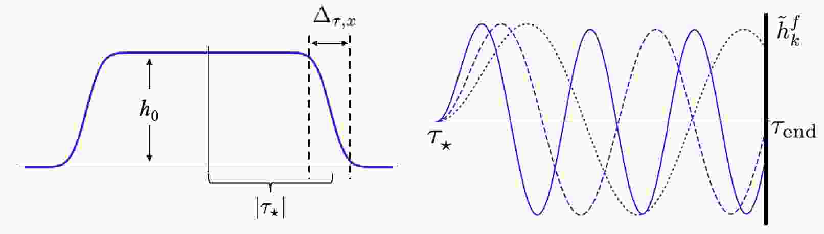
$ ' $ indicates derivatives with respect to the conformal time τ,$ G_N $ is Newton's gravity constant, and$ \sigma_{ij} $ is the transverse, traceless part of the energy momentum tensor. In this paper, we assume that the Hubble parameter ($ H_{\rm int} $ ) during inflation is a constant. Subsequently, we obtain$a(\tau) = - 1/H_{\rm inf} \tau$ . The problem contains several important time scales:$ \tau_\star $ is the time of bubble collision and generation of the GW. The inflation ends at$ \tau_{\rm end} $ . We denote the conformal time duration and the co-moving spatial spread of the bubble collision event as$ \Delta_{\tau,x} $ .$ \Delta_{\tau,x} \ll |\tau_\star| $ by assumption of instantaneous and local sources that occurred during inflation. The modes of interest to us are all outside the horizon at the time when inflation ends,$ k|\tau_{\rm end}| \ll 1 $ , where k is the co-moving momentum. -
We focus on three regimes with qualitatively different features.
$ \bullet \ |\tau_\star|^{-1} < k < \Delta_{\tau,x}^{-1} $ . In this regime, we can ignore the spatial inhomogeneity caused by the bubbles and consider the bubble collisions as instantaneous sources. Therefore, the bubble collisions can be approximated as delta function sources:$ \begin{array}{*{20}{l}} \tilde\sigma_{ij} \approx \tilde T_{ij}^{(0)}a^{-3}(\tau_\star) \delta(\tau - \tau_\star) \ , \end{array} $

(2) where, in this regime,
$ \tilde T_{ij}^{(0)} $ is independent of$ {\bf {k}} $ [43].During inflation and after the bubble collision,
$|\tau_\star| \gg |\tau | > |\tau_{\rm end}|$ , we have (after Fourier transformation and suppressed$ i,j $ indices)$ \begin{aligned}[b] \tilde{h}_{{\bf {k}}} (\tau) \approx & -\frac{16\pi G_N H_{\rm inf} \tilde T^{(0)} \tau }{k} \left[ \left( \frac{1}{k \tau } - \frac{1}{k \tau_\star} \right) \cos k(\tau-\tau_\star) \right. \\ &+ \left.\left(1+ \frac{1}{k^2(\tau \tau_\star)} \right) \sin k(\tau - \tau_\star ) \right] \ . \end{aligned} $

(3) In position space, when
$ k^2 \tau\tau_\star \ll 1 $ ,$ h(\tau,{\bf x}) $ is approximately$ 4 G_N H_{\rm inf} \tilde T^{(0)}|\tau_\star|^{-1} \Theta(\tau -\tau_\star - |{\bf x}-{\bf x_\star}|) $ , which is uniform over a density ball with radius$ |\tau_\star| $ , as shown in the left panel of Fig. 1. At the end of inflation, the universe is filled with such GW balls. In this regime, we can ignore the terms suppressed by$ (k \tau_\star)^{-1} $ in Eq. (3). After the GW is produced at$ \tau \approx \tau_\star $ , it continues to oscillate until it exits the horizon at$ k |\tau| \approx 1 $ when its phase begins to freeze. The GW then evolves to the end of the inflation, and with$ k\tau_{\rm end} \rightarrow 0 $ , its value is frozen to
Figure 1. (color online) Left: configuration of bound state of the GW in the inflation era. Right: Fourier modes of the GW during inflation from
$ \tau_\star $ to$ \tau_{\rm end} $ .$ \tilde h_{{\bf {k}}}^{f} = - \frac{16\pi G_N H_{\rm inf} \tilde T^{(0)}}{k^2} \left(\cos k\tau_\star - \frac{\sin k\tau_\star}{k \tau_\star}\right) \ . $

(4) Since
$ k |\tau_\star| > 1 $ , we can neglect the term proportional to$ \sin k\tau_\star/k\tau_\star $ . Hence,$ \tilde h^f_{{\bf {k}}} \sim \cos k \tau_\star $ , as shown in the right panel of Fig. 1.The GW begins to oscillate again after re-entering the horizon, with
$ \tilde{h}_{{\bf {k}}}^f $ as the initial condition. For example, if we assume that the universe evolves into the radiation domination (RD) immediately after inflation,$ \tilde h_{{\bf {k}}}(\tau) = \tilde h^f_{{\bf {k}}} \times \frac{\sin k\tau}{k\tau} \ . $

(5) Hence,
$ \tilde{h}_{{\bf {k}}}(\tau) \propto \cos (k \tau_\star) $ . The energy density of the GW has the form$ \rho_{\rm GW} \sim \frac{1}{a^2(\tau)} \int \frac{{\rm d}^3k}{(2\pi)^3} |\tilde h'_{{\bf {k}}}(\tau)|^2 \ . $

(6) As a result, deeply inside the horizon (
$ k\tau \gg 1 $ ), we have$ \frac{{\rm d}\rho_{\rm GW}}{{\rm d}\log k} \sim \frac{1}{k} \left(\cos k \tau_\star - \frac{\sin k\tau_\star}{k \tau_\star} \right)^2 \approx \frac{1}{k} \cos^2 k \tau_\star \ . $

(7) We observe that the GW has a distinct oscillatory feature in the frequency space, with a period of
$ \pi / \tau_\star $ . This feature results from the instantaneous nature of the GW production, which sets up a GW spectrum proportional to$ \cos k|\tau_\star| $ at the end of the inflation. The GW energy density also has an overall factor of$ k^{-1} $ [41], since the modes with a longer wavelength redshift less before exiting the horizon. An illustration of the GW spectrum is shown in Fig. 2.
Figure 2. (color online) Illustration of the shape of the GW spectrum produced by an instantaneous source during inflation.
$ \bullet \ k <\tau_{\star}^{-1} $ . In this regime, we can ignore the details of the GW source and consider it as a delta function in space-time. Hence, Eq. (3) still applies. In the limit$k|\tau_{\rm end}| \ll k|\tau_\star| \ll 1$ , from Eq. (4),$ h_f^k $ is independent of k at the leading order. From Eq. (7), we have${\rm d} \rho_{\rm GW} /{\rm d} \log k \propto k^3$ , also shown in Fig. 2, which is similar to the case of producing the GW from an instantaneous source in the RD [43, 44].$ \bullet \ k \gtrsim \Delta_{\tau,x}^{-1} $ . In this regime, we have$ k |\tau_{\star}| \gg 1 $ . The details of the bubble collision become essential, and we require numerical simulations to obtain the shape of the signal. At such small scales, the curvature of the space-time is not important when the GW is produced. However, the inflation effect distorts the GW spectrum. As a result, the energy density behaves as$ \frac{{\rm d}\rho_{\rm GW}}{{\rm d}\log k} \sim k^{-4} \frac{{\rm d}\rho_{\rm GW}^{\rm flat}}{{\rm d}\log k_p} \ , $

(8) where
$ k_p = k/a $ is the physical momentum.${{\rm d}\rho_{\rm GW}^{\rm flat}}/{{\rm d}\log k_p}$ is the GW spectrum produced from the same source in the Minkowski space-time. The distortion factor$ k^{-4} $ results from the$ k^2 $ factor in the denominator of Eq. (4).${{\rm d}\rho_{\rm GW}^{\rm flat}}/{{\rm d}\log k_p}$ often decreases as$ k_p^{-r} $ , with$ r = 1 $ for bubble collisions [45]. Therefore, for a GW produced by approximately instantaneous sources during inflation, the UV part of the spectrum decreases as$ k^{-5} $ .Owing to the finite duration (of
$ {\mathcal O}(\Delta_{\tau,x}) $ ) of the sources, the oscillatory pattern in the UV part,$ k \gtrsim \Delta_{\tau,x}^{-1} $ would be smeared out. This finite size effect should also blunt the oscillation pattern in the regime$ |\tau_\star|^{-1} < k < \Delta^{-1}_{\tau,x} $ . A detailed simulation can determine precisely how the spectrum is smeared. For an observer in today's universe, the GWs originating from different directions correspond to uncorrelated sources during inflation. Thus, we can simply sum their strengths. Therefore, we can use a window function to mimic this effect by replacing the factor$ (\sin k\tau_\star/k\tau_\star - \cos k\tau_\star)^2 $ in Eq. (7) with$(2\Delta)^{-1}\int_{\tau_\star-\Delta}^{\tau_\star+\Delta} {\rm d}\tau_\star' (\sin k\tau_\star'/ k\tau_\star' - \cos k\tau_\star')^2$ , where$ \Delta\sim\Delta_{\tau,x} $ embodies the duration of the source.Combining the above analysis, the general form of the GW spectrum when it is back into the horizon in the RD can be expressed as
$ \frac{{\rm d}\rho_{\rm GW}}{{\rm d}\log k} = \frac{a^4(\tau_{\rm end})}{a^4(\tau)} {\cal S}(k_p) \frac{{\rm d}\rho_{\rm GW}^{\rm flat}}{{\rm d}\log k_p} \ , $

(9) where
$ {\cal S}(k_p) $ is$ \begin{aligned}[b] {\cal S}(k_p) =& \frac{H_{\rm inf}^4}{k_p^4}\Bigg\{\frac{1}{2} + \frac{\cos(2k_p/H_{\rm inf}) \sin(2k_p \Delta_p)}{4k_p \Delta_p}\\&+ \frac{1}{4k_p \Delta_p} \Bigg( \frac{1 - \cos(2k_p/H_{\rm inf} - 2k_p \Delta_p)}{k_p/H_{\rm inf} - k_p \Delta_p} \\&- \frac{1 - \cos(2k_p/H_{\rm inf} + 2k_p \Delta_p)}{k_p/H_{\rm inf} + k_p \Delta_p}\Bigg)\Bigg\}. \end{aligned} $

(10) $ \Delta_p = a^{-1}(\tau_\star) \Delta $ is the physical duration of the source. -
To determine the strength and the frequency of the GW today, we must study a specific model. We assume that the backreaction from the spectator sector that underwent the phase transition to the evolution of the inflaton field is negligible. For a signal to be detectable, the latent heat density released during the phase transition should be larger than
$ H_{\rm inf}^4 $ . Hence, the plasma, with an energy density that can be estimated as$ T_{\rm GH}^4 \sim H_{\rm inf}^4/(2\pi)^4 $ , is negligible. As a result, the production of the GW is dominated by bubble collisions. A comprehensive description of bubble collision and GW production is available in Ref. [45]. During bubble collision, the parameter$\beta \equiv - {\rm d} S_4/{\rm d}t$ determines the size of the bubble and wavelength of the GW, where$ S_4 $ is the action of the bounce at the end of the phase transition. Here, we use$ S_4 $ since the phase transition rate is dominated by quantum tunneling. For the phase transition to complete during inflation, we assume$ \beta \gg H_{\rm inf} $ . When$ \beta \approx H_{\rm inf} $ , a numerical simulation is required, which is beyond the scope of this paper. The discussions of models in which first-order phase transition can occur during inflation and the possible range of$ \beta/H $ are presented in the Appendix.For an instantaneous reheating and followed by RD, all the energy of the inflaton field converts into the radiation energy. Hence, today's relative abundance of GW can be expressed as
$ \Omega_{\rm GW}(k_{\rm today}) = \Omega_R \times {\cal S}(k) \times \frac{\Delta\rho_{\rm vac}}{\rho_{\rm inf}} \frac{{\rm d}\rho^{\rm flat}_{\rm GW}}{\Delta\rho_{\rm vac} {\rm d}\log k_p} \ , $

(11) where
$ \Omega_R $ is today's abundance of radiation, and$ \Delta\rho_{\rm vac} $ is the latent energy density of the phase transition sector. The last factor is the flat space-time spectrum of the GW:$ \frac{{\rm d}\rho^{\rm flat}_{\rm GW}}{\Delta\rho_{\rm vac} {\rm d}\log k_p} = \kappa^2 \frac{\Delta\rho_{\rm vac}}{\rho_{\rm inf}} \left(\frac{H_{\rm inf}}{\beta}\right)^2 \Delta(k_p/\beta) \ , $

(12) where
$ \kappa = 1 $ if the energy density of the plasma is negligible, and the simulation result yields$ \Delta(k_p/\beta) = \tilde\Delta \times \frac{3.8\tilde k_p k_p^{2.8}}{\tilde k_p^{3.8} + 2.8k_p^{3.8}} \ , $

(13) where
$ \tilde k_p = 1.44\beta $ and$ \tilde \Delta = 0.077 $ . In the calculation of the GW spectrum, we use$ \beta^{-1} $ to estimate$ \Delta_p $ in$ {\cal S} $ . The signal strength is suppressed by the factor$ (H_{\rm inf}/k_p)^4 $ owing to the dilution during inflation as shown in Eq. (10). A qualitative understanding of this factor is provided in the Appendix.Finally, the observed GW frequency is
$ \frac{f_{\rm today}}{f_\star} = \frac{a(\tau_\star)}{a_1} \left(\frac{g_{*S}^{(0)}}{g_{*S}^{(R)}}\right)^{1/3} \frac{T_{\rm CMB}}{\left[\left(\dfrac{30}{g_*^{(R)} \pi^2}\right) \left( \dfrac{3 H_{\rm inf}^2}{8\pi G_N} \right)\right]^{1/4}} \ , $

(14) where the superscript
$ (R) $ indicates the values of parameters at the reheating temperature. Owing to the distortion induced by inflation, the position of the highest peak of the spectrum corresponds to$ k_p \approx H_{\rm inf} $ . As a result, assuming$ g_{*S}^{(R)} = g_*^{(R)} \approx 100 $ , the frequency of highest peak today is$ \tilde f_{\rm today} = 1.1\times10^{11} {\; \rm Hz} \left(\frac{H_{\rm inf}}{m_{\rm pl}}\right)^{1/2} \left(\frac{a_\star}{a_1} \right) . $

(15) Using high scale inflation as an example,
$ (H_{\rm inf}/m_{\rm pl})^{1/2} \sim 10^{-3}-10^{-4} $ . Detectors based on the pulsar timing technology, such as EPTA [9], IPTA [10], and SKA [11], are sensitive to GWs with frequencies of approximately$ 10^{-8} $ Hz. As shown in Eq. (15), they can probe the GWs produced at the era of about 40 e-folds before the end of inflation, as shown by the blue curves in Fig. 3. The space-based detectors, such as LISA [2], eLISA [1], DECIGO [3], BBO [7, 8], ALIA [6], TianQin [4], and Taiji [5], are sensitive to frequencies at approximately$ 10^{-2} $ Hz, corresponding to about 20 e-folds before the end of inflation, as shown by the magenta and red curves in Fig. 3. The proposed ground-based detectors (e.g., the Einstein Telescope [15] and the Cosmic Explorer [16]) are sensitive to GWs with frequencies of$ 10-10^4 $ Hz, which correspond to about 15 e-folds from the end of inflation. They can detect the signal of the phase transition if$ \beta \approx 2 H_{\rm inf} $ . However, as shown by the purple dotted curve in Fig. 3, the oscillatory feature is expected to be smeared out since$ \Delta_p \sim H_{\rm inf}^{-1} $ .
Figure 3. (color online)
$ \Omega_{\rm GW} $ as a function of f. The blue, magenta, red, and purple curves are for$ N_e = 38 $ , 25, 21, and 15, respectively. The values of$ \beta/H_{\rm inf} $ for each curve are shown in the legend. For all the curves,$ H_{\rm inf} = 10^{12} $ GeV and$ \Delta\rho_{\rm vac}/\rho_{\rm inf} = 0.3 $ . The curve for the sensitivity of BBO phase 2 (BBO2) is obtained from [46]. Curves for sensitivities of other detectors are obtained from [47]. -
If the phase transition occurs about 60 e-folds before the end of inflation, it would leave an imprint on the CMB B-mode power spectrum [40]. Since the strength of the GWs depends on
$ H_{\rm inf} $ only through the ratio$ H_{\rm inf}/\beta $ , as shown in Eqs. (11) and (12), a sizable B-mode spectrum can be observed from the CMB even in low scale inflation models.We simulate the B-mode power spectra induced by first-order phase transitions using the class package [49]. The result is shown in Fig. 4, where
$ \beta/H_{\rm inf} $ and$ \Delta\rho_{\rm vac}/\rho_{\rm inf} $ are fixed to be$ 30 $ and$ 0.1 $ , respectively. The frequency of GW depends on$ H_{\rm inf} $ , which we have selected to be$ H_{\rm inf} = 10^{12} $ GeV. The solid, dashed, and dot-dashed curves are the spectra for$ N_e $ = 59, 58, and 57, respectively. Small wiggles induced by the oscillatory pattern are observed in the GW power spectrum. Since the spherical harmonics are not orthogonal to the Fourier modes, the oscillatory pattern is smeared. The amplitude of the oscillation is only about 10% of the total. As a comparison, the black dotted curve in Fig. 4 shows the B-mode power spectrum produced by quantum fluctuations during inflation with the tensor-scalar ratio$ r = 0.003 $ , which can be reached by the CMB-S4 at the$ 5\sigma $ level [19]. Of course, the inflationary history in this era will also be probed and potentially constrained by other CMB and large scale structure observables. The search for the GW signal discussed here will provide complementary information. We will provide a more detailed discussion in a separate paper.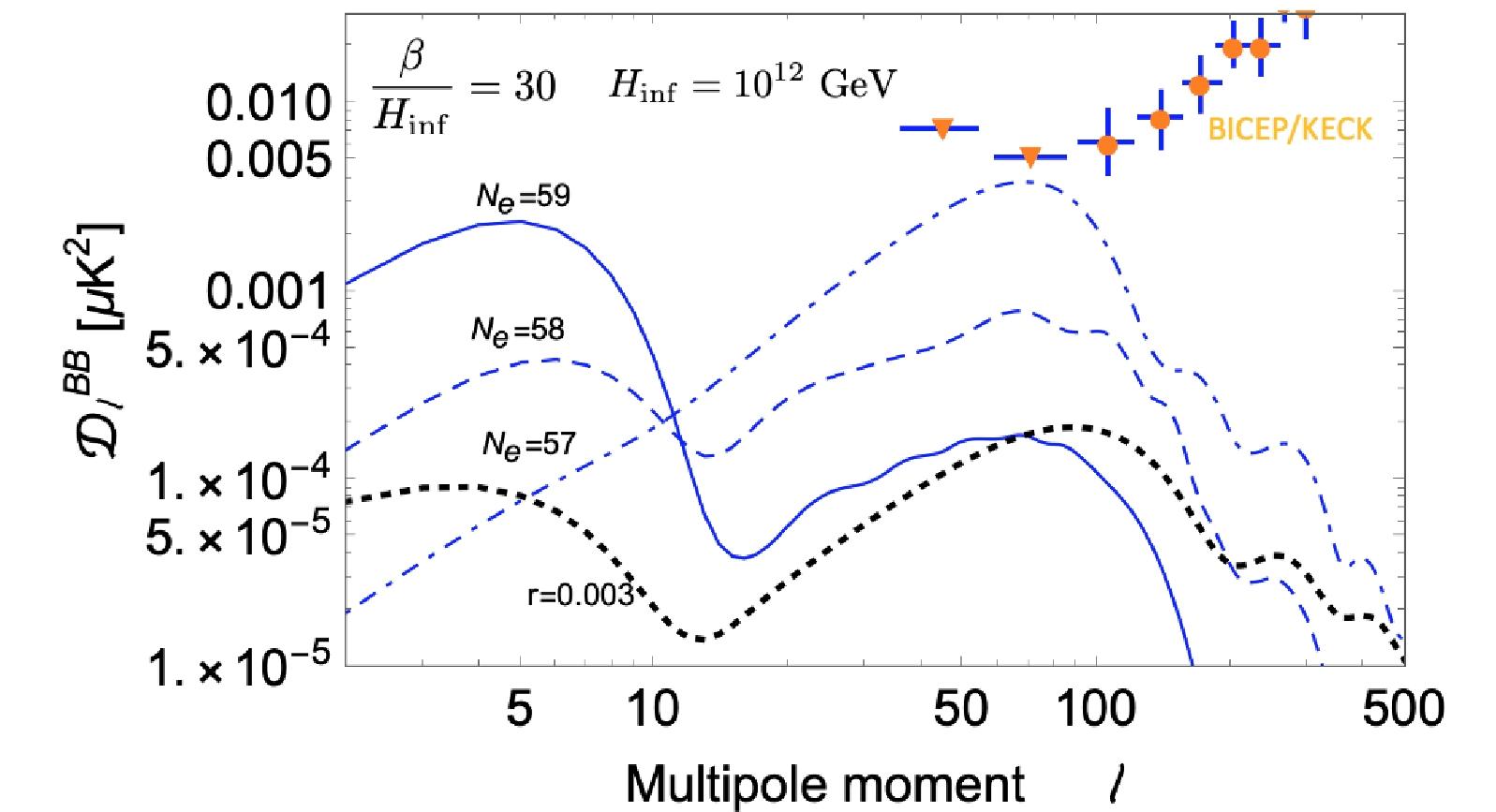
Figure 4. (color online) B-mode power spectra from the bubble collision at
$ N_e = 59, 58, 57 $ during inflation with$ \beta / H_{\rm inf}=30 $ and$ H_{\rm inf}=10^{12} $ GeV.$ \Delta\rho_{\rm vac}/\rho_{\rm inf}=0.1 $ . The spectrum generated from quantum fluctuations for tensor-scalar ratio$ r=0.003 $ is also shown. The orange dots and downward triangles are data from the BICEP/Keck array [48]. -
The GW spectrum produced from instantaneous sources during inflation has an oscillatory feature, as shown in Figs. 3 and 4, and can be detected by future GW detectors, whereas most of the spectra of GWs from sources after inflation can be fit using power laws or breaking power laws (a comprehensive review of the properties of cosmically produced GW after inflation is available in Ref. [50]). Therefore, this feature enables us to distinguish it from GWs generated by sources after inflation. From the frequency of the oscillation in the spectrum, we can learn the energy scale of the phase transition in the unit of the Hubble expansion rate during inflation. The information of the time the phase transition occurred is encoded in the frequency of the GWs. Fig. 5 shows the future reaches of LISA, DECIGO, BBO, and SKA projects for
$ \Delta\rho_{\rm vac}/\rho_{\rm inf} = 0.3 $ and$ H_{\rm inf} = 10^{12} $ GeV.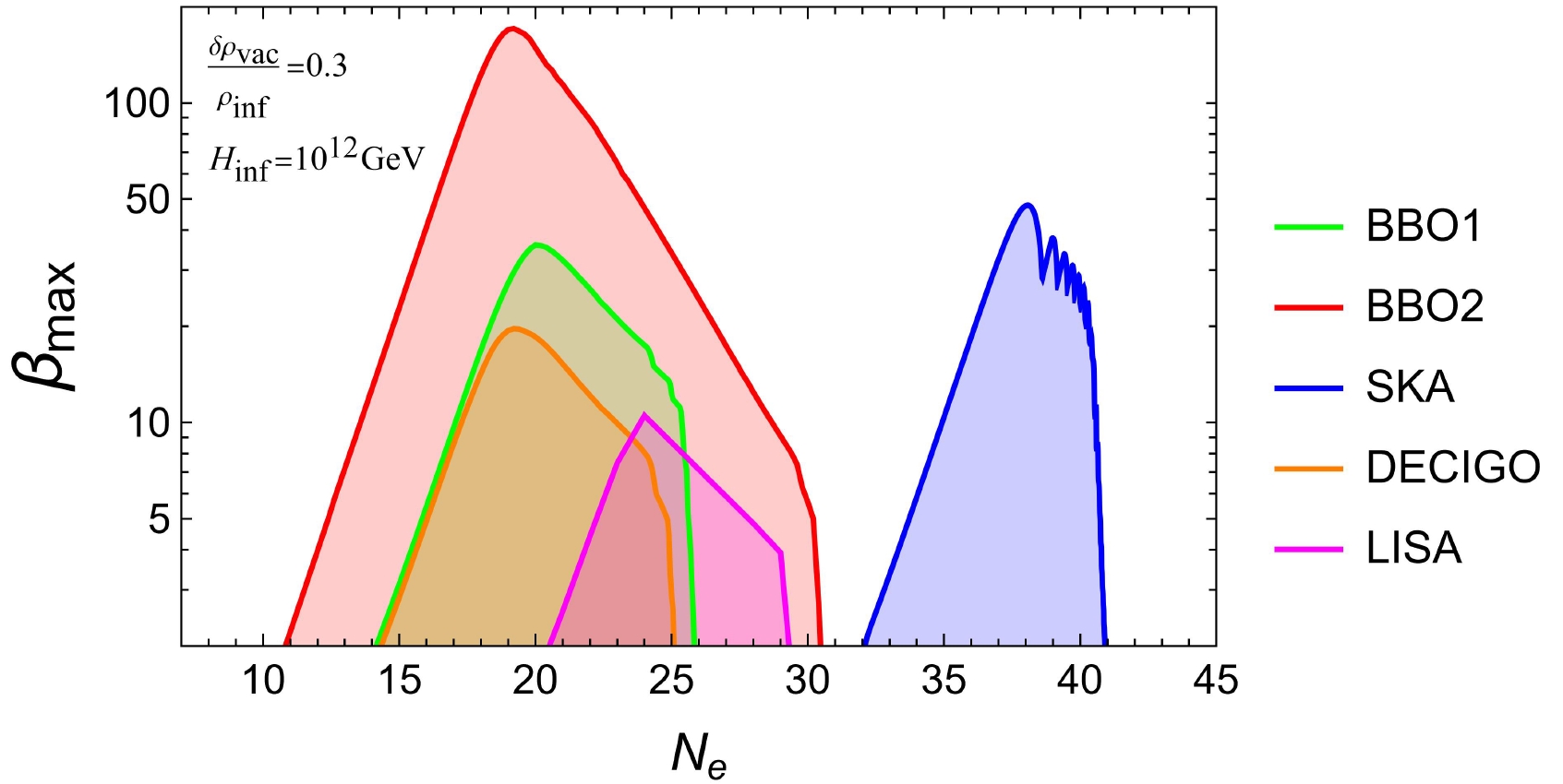
For the inflationary history outside the ten e-folds around the CMB era, there is no direct measurement of the power spectrum. Hence, the evolution there can differ significantly from the simple form assumed in this paper. Moreover, if a first-order phase transition occurred at approximately
$ N_e \geq 10 $ , the details of the oscillatory spectrum can aid us in mapping out this part of "missing history." A detailed investigation of this subject will be presented in a separate paper.If the phase transition occurred in the regime that can be detected in the CMB, the mass of the fields in the spectator sector must be larger than
$ H_{\rm inf} $ such that their perturbations induced by the phase transition will decay rapidly after evolving out of the horizon. In contrast, if the phase transition occurs in the missing history and light degrees of freedom exist in the spectator sector, the perturbations may induce primordial black holes or dark blobs, resulting in additional signals in the future. -
In this section, we provide simple examples that first-order phase transitions can occur during inflation. As discussed in the main text, the general scheme is that the first-order phase transition occurs in a spectator sector, which for simplicity, we take to be a scalar field σ. We consider the following examples of the spectator potential together with a coupling to the inflaton field ϕ:
$ \begin{aligned}[b] V_1(\phi,\sigma) =& -\frac{1}{2} (\mu^2 - c^2 \phi^2 ) \sigma^2 + \frac{\lambda}{4}\sigma^4 + \frac{1}{8 \Lambda^2 } \sigma^6 \\ V_2(\phi,\sigma) =& -\frac{1}{2} (\mu^2 - c^2 \phi^2 ) \sigma^2 + \frac{\lambda}{4}\sigma^4 + \frac{\kappa}{4} \sigma^4\log\frac{\sigma^2}{\Lambda^2} \\ V_3(\phi,\sigma) =& -\frac{1}{2} (\mu^2 - c^2 \phi^2) \sigma^2 + \frac{\lambda}{3}{\cal E}\sigma^3 + \frac{\kappa}{4} \sigma^4 \ . \end{aligned} \tag{A1}$

We assume that during inflation, the field value of ϕ becomes smaller. For
$ \mu^2 > 0 $ ,$ \lambda < 0 $ , and$ c^2 >0 $ , first-order phase transition can occur. In the models in Eq. (A1), we can define an effective mass square$ \mu_{\rm eff}^2 \equiv - (\mu^2 - c^2 \phi^2) $ . With the rolling the inflaton field, the effective mass evolves from positive to negative. With$ \lambda<0 $ , there would be a barrier in the potential. Hence, the phase transition would be first-order. Thus, the first-order phase transition can occur in all three models, as shown in Fig. A1. A detailed analysis of the potentials is in parallel to the electroweak phase transition with the temperature T replaced by$ c\phi $ and is provided in Ref. [51]. There can also be models in which the evolution of the inflaton field changes the values of the couplings in the spectator sector. For example,
Figure A1. (color online) Shapes of the potentials as a function of σ for different choices of ϕ.
$ {\cal L}_\sigma = - \left(1 - \frac{\phi^2}{\Lambda^2}\right)\frac{1}{4g^2} G^a_{\mu\nu} G^{a\mu\nu} \ , \tag{A2} $

where G is the field strength of some non-Abelian gauge group. Such a change can trigger a phase transition. Whether the phase transition is first-order depends on other parameters such as number of colors and flavors. In this paper, we indicate that if the phase transition is of first-order, we may observe an oscillatory pattern related to it.
-
In this section, we provide estimates of the energy scales and other parameters of the inflation and the spectator sector to generate first-order phase transition while preserving the success of the inflation. We also estimate the size of the bubble, justifying the range assumed in the main text.
Let us consider de Sitter inflation. The metric is
$ {\rm d}\tau^2 = {\rm d}t^2 - {\rm e}^{2Ht} ({\rm d}x^2 + {\rm d}y^2 + {\rm d}z^2) \ .\tag{B1} $

The bubble nucleation rate per physical volume can be written as
$ \frac{\Gamma}{V_{\rm phy}} = C m_\sigma^4 {\rm e}^{-S_4} \ , \tag{B2} $

where
$ m_\sigma $ is the typical energy scale of the spectating sector, and$ S_4 $ is the bounce action. Therefore, the bubble nucleation rate per comoving volume at time t can be expressed as$ \frac{\Gamma}{V} = {\rm e}^{3 H t} C m_\sigma^4 {\rm e}^{-S_4} \ . \tag{B3} $

Now, let us assume the bubbles expand with the speed of light. That means the point on the bubble wall evolves along a null geodesic curve. We have
${\rm d}t = {\rm e}^{Ht} {\rm d}r$ for the bubble created at the origin of the space. Thus, we easily observe that for a bubble nucleated at$ t' $ , its comoving radius at t can be expressed as$ R(t,t') = \frac{1}{H} ({\rm e}^{-H t'} - {\rm e}^{-H t}) \ . \tag{B4}$

Thus, the fraction of the space that remains at the false vacuum at time t can be expressed as [52]
$ \begin{aligned}[b] {\cal P} (t) =& \exp\Bigg[ - \int_{-\infty}^{t} {\rm d}t' \frac{4 \pi}{3 H^3} \\ & \times ({\rm e}^{-H t'} - {\rm e}^{-H t})^3 {\rm e}^{3H t'} C m_\sigma^4 {\rm e}^{-S_4(t')} \Bigg] \ . \end{aligned}\tag{B5} $

Now, the necessary condition for the phase transition to finish at t is that the exponential part of
$ {\cal P}(t) $ can achieve order of unity. Therefore, we require$ \int_{-\infty}^{t} {\rm d}t' \frac{4\pi}{3 H^3} ({\rm e}^{-H t'} - {\rm e}^{-H t})^3 {\rm e}^{3H t'} C m_\sigma^4 {\rm e}^{-S_4(t')} \sim {\cal O}(1) \ . \tag{B6} $

The bounce action
$ S_4 $ at$ t' $ can be expanded as$ S_4(t') = S_4(t) + \frac{{\rm d} S_4(t)}{{\rm d}t} (t' - t) \equiv S_4 (t) - \beta (t' - t) \ . \tag{B7} $

Therefore, the condition for the phase transition to complete is
$ \begin{aligned}[b] {\cal O}(1) \sim & C m_\sigma^4 {\rm e}^{-S_4(t)} \frac{4\pi}{H^3} \int_{-\infty}^t {\rm d} t' \left( 1 - {\rm e}^{- H (t - t')}\right)^3 {\rm e}^{-\beta(t - t')} \\ \approx & C m_\sigma^4 {\rm e}^{-S_4(t)} \frac{8\pi}{\beta (\beta+H)(\beta + 2H)(\beta + 3H) } \\ \approx & 8\pi C {\rm e}^{-S_4(t)} \frac{m_\sigma^4}{\beta^4} \ , \end{aligned}\tag{B8} $

where in the last step
$ \beta \gg H $ is assumed. Therefore, the requirement for first-order phase transition to complete at$ t_0 $ is$ S_4(t_0) \approx \log \left(\frac{m_\sigma^4}{ \beta^4}\right) \ . \tag{B9} $

The requirement that the phase transition is strong first-order requires
$ S_4 \gg 1 $ , which indicates$ m_\sigma^4 \gg \beta^4 \ . \tag{B10} $

In contrast, the energy density in the spectating sector must be smaller than the total energy driven the inflation. We have
$ m_\sigma^4 \ll M_{\rm pl}^2 H^2 \ . \tag{B11} $

Therefore, we require
$ \left[\left(\frac{\beta}{H} \right)^4 H^2\right] H^2 \ll m_\sigma^4 \ll M_{\rm pl}^2 H^2 \ . \tag{B12}$

In the following, we can observe that the typical value of
$ \beta/H $ is about$ {\cal O}(10) - {\cal O}(100) $ . Therefore, for reasonable values of H, we always have$ \beta^4 \ll H^2 M_{\rm pl}^2 \ . \tag{B13} $

As a result, we can always build a model for first-order phase transition to complete during inflation as long as the condition
$ \beta/ H \gg 1 $ is fulfilled. The evolution of$ 1- {\cal P} $ is shown in Fig. B1, and we can observe that as long as long as the condition$ \beta/H \gg 1 $ is fulfilled, the phase transition can complete within less then one e-fold.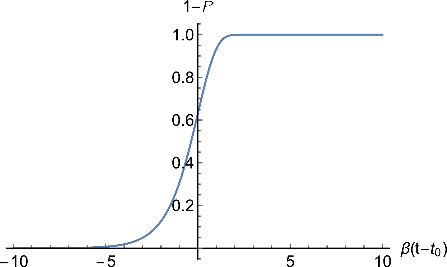
Figure B1. (color online) Evolution of the fraction of the space occupied by the true vacuum.
-
In a first-order phase transition, the typical radius of the bubbles at the end of the phase transition can be estimated as
$\beta^{-1} = |{\rm d}S_4/{\rm d}t|^{-1}$ . We have$ \begin{aligned}[b] \beta =& \left|\frac{{\rm d} S_4}{d t}\right| = \left|\frac{{\rm d} S_4}{{\rm d} \mu_{\rm eff}^2}\right| \left|\frac{{\rm d}\mu_{\rm eff}^2}{{\rm d}t} \right| \\ =& \left|\frac{{\rm d} S_4}{{\rm d}\log \mu_{\rm eff}^2} \right| \left|\frac{{\rm d}\mu_{\rm eff}^2}{\mu_{\rm eff}^2{\rm d}t} \right|= I_1 S_4 \left|\frac{2 \dot\phi}{\phi - \dfrac{\mu^2}{c^2\phi}} \right| \ , \end{aligned}\tag{B14} $

where
$ I_1 = \frac{1}{S_4} \left|\frac{{\rm d} S_4}{{\rm d}\log\mu_{\rm eff}^2} \right| \ , \tag{B15} $

can be calculated numerically using CosmoTransitions [53], and the results show that the value of
$ I_1 $ can vary from 0.2 to 5.Therefore, we obtain
$ \frac{\beta}{H} = I_1 S_4 (2\epsilon)^{1/2} \times \frac{M_{\rm pl}}{|\phi - \dfrac{\mu^2}{c^2\phi}|} \ . \tag{B16} $

In slow-roll single field models, we have the simple relation [36]
$ \int_{\phi_{\rm end}}^{\phi_{\rm PT}} \frac{{\rm d}\phi}{\sqrt{2\epsilon} M_{\rm pl}} = N_{\rm e} \ , \tag{B17} $

where
$ N_{\rm e} $ is defined as the number of e-folds before the end of inflation. Therefore, if we use the range of ϕ to estimate the value of ϕ at the moment of the phase transition and assume$ \epsilon $ does not evolve much after the phase transition, we have$ \frac{\beta}{H} \approx \frac{{\rm d}S_4}{{\rm d}\log\mu_{\rm eff}^2}\times \frac{1}{N_e|1 - \dfrac{\mu^2}{c^2 \phi^2}|} \ . \tag{B18} $

In the phase transition region, since a small bounce is usually required, a cancelation often occurs between the two terms in
$ \mu_{\rm eff}^2 $ . For example, for$ V_1 $ and$ V_2 $ , during the phase transition, the ratio$ \mu_{\rm eff}^2/\Lambda^2 $ changes from order one to about$ 10\% $ . Therefore, it is very probable that in the framework of slow-roll phase transition, the value of$ \beta/H $ is about$ {\cal O} $ (10) to$ {\cal O} $ (100). -
To illustrate the completeness of the phase transition, we performed some numerical simulations of the expansion of the bubbles in de Sitter space. We begin the simulation of bubble nucleation at
$ t_0 $ when we have$ \Gamma/V_{\rm phy} = H^4 $ , namely, one bubble is nucleated at each Hubble patch in one e-fold. The condition that$ S_4 \gg 1 $ requires that$ m_\sigma^4 \gg H^4 $ . This condition is weaker than Eq. (27) and therefore can be fulfilled as discussed in the last subsection. Subsequently, we expand$ S_4 $ as$S_4(t_0) - \beta(t - t_0)$ . We then randomly generate bubbles according to the nucleation rate. After nucleation, we assume that the bubbles expand with the speed of light. The evolution of the fraction occupied by the new vacuum is shown in Fig. B2, where the blue and green curves are for$ \beta/H = 30 $ and 15. We can observe that in both cases the time durations of the phase transition (from 10% to 90% as shown in Fig. B2) are significantly smaller than$ H^{-1} $ .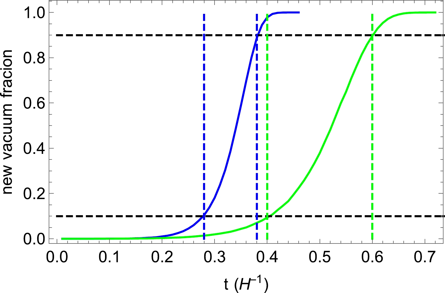
Figure B2. (color online) Numerical simulation of the occupation fraction of the new vacuum for
$ \beta/H = 30 $ (blue) and$ \beta/H = 15 $ (green).When the phase transition is about to complete (e.g., when the occupation faction of the new vacuum is approximately 90% at
$ t \approx 0.39 H^{-1} $ for$ \beta/H = 30 $ and$ t\approx 0.6 H^{-1} $ for$ \beta/H = 15 $ ), the distribution of the physical radius of the bubbles are shown in Fig. B3. We observe that the peak positions of the radius distributions in both cases are about$ \beta^{-1} $ . The typical bubble configurations when the phase transition is about to complete are shown in Fig. B4. We observe that the size of the bubbles for$ \beta/H = 30 $ is significantly smaller than that for$ \beta/H = 15 $ .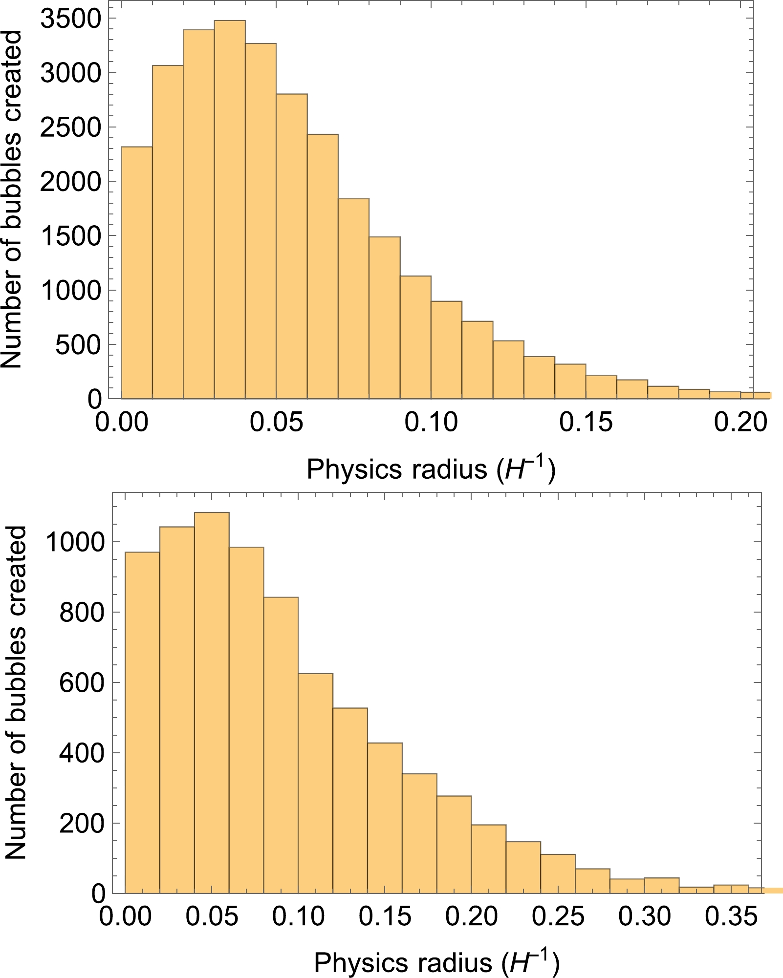
Figure B3. (color online) Distributions of the physical radius of bubbles when the occupation faction of the new vacuum is about 90% for
$ \beta/H = 30 $ (left) and$ \beta/H = 15 $ (right). The vertical axis shows the number of bubbles in a comoving volume of$ 8 H^{-3} $ in each radius bin.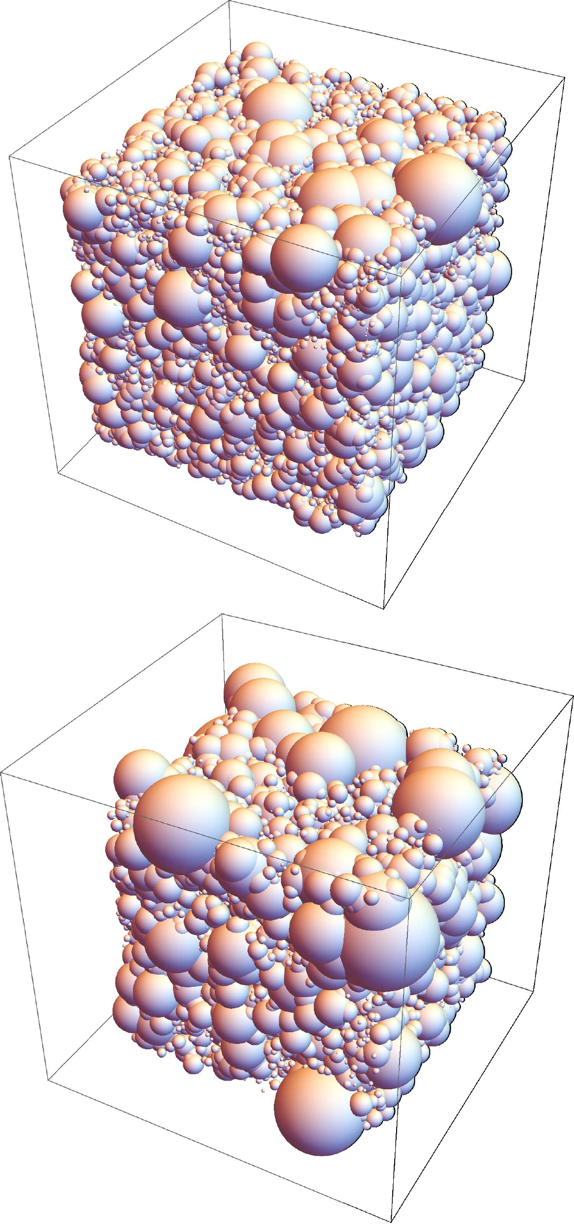
Figure B4. (color online) Typical bubble configurations at the completion of the phase transition for
$ \beta/H = 30 $ (left) and$ \beta/H = 15 $ (right) in the$ 2H^{-1}\times2H^{-1}\times 2H^{-1} $ comoving box. -
When the GW is generated, the subsequent evolution is a known phenomenon. In the main text, we quote the result of the solution of relevant equations of motion. Here, we provide a scaling argument to understand the parametric dependence of the signal strength on the relevant scales of the model.
For a GW mode with physical momentum
$ k_p $ at the moment it is produced, its energy density redshifts with$ a^{-4} $ before it exits the horizon when$ k_p \sim H $ . When it is outside the horizon before the end of inflation, the field value$ h_{ij} $ as defined in the manuscript remains constant, while the momentum still redshifts as$ a^{-1} $ . As a result, in this period, the GW energy density redshifts as$ a^{-2} $ . After the end of inflation, when the GW mode is still outside the horizon, for the same reason, the energy density becomes$ a^{-2} $ . When it evolves back inside the horizon, its energy density redshifts as$ a^{-4} $ again. Therefore, the energy density of the GW when it returns into the horizon can be expressed as$ \rho_{\rm GW}(t) \approx \rho_{\rm GW}^0 \times \left( \frac{H}{k_p} \right)^4 \left( \frac{a_1}{a_2} \right)^2 \left( \frac{a_2}{a_3} \right)^2 \left( \frac{a_3}{a(t)} \right)^4 \ , \tag{C1}$

where
$ a_1 $ is the scale factor when the mode evolves outside the horizon,$ a_2 $ when inflation ends,$ a_3 $ when the mode reenters the horizon. After inflation, in the radiation dominated era, the Hubble parameter is$ H \sim \frac{T^2}{M_{\rm pl}} \sim a^{-2} \ . \tag{C2} $

Assuming H is a constant during inflation, we have
$ \frac{a_1}{a_2} = \frac{a_2}{a_3} \ . \tag{C3} $

The energy density can be rewritten as
$ \begin{aligned}[b] \rho_{\rm GW}(t) \approx& \rho_{\rm GW}^0 \times \left( \frac{H}{k_p} \right)^4 \left( \frac{a_2}{a_3} \right)^4 \left( \frac{a_3}{a(t)} \right)^4 \\ =& \rho_{\rm GW}^0 \times \left( \frac{H}{k_p} \right)^4 \left( \frac{a_2}{a(t)} \right)^4 \ . \end{aligned}\tag{C4} $

In this paper, we study the case in which most of the energy of the inflaton potential is converted into radiation. Hence, after inflation, the energy of the radiation evolves as
$ \rho_{\rm R} \sim \rho_{\rm inf} \times \left(\frac{a_2}{a(t)}\right)^4 \ . \tag{C5} $

Finally, today's abundance of GWs is
$ \Omega_k = \Omega_R \times \frac{{\rm d}\rho_{\rm GW}}{\rho_{R} {\rm d}\log k } \sim \left( \frac{H}{k_p} \right)^4 \ . \tag{C6} $

Therefore, the GW signal is only diluted by a factor of
$ (H/k_p)^4 $ . This factor is explicitly shown in the$ {\cal S} $ factor in Eq. (10) of the manuscript. During phase transition, the typical value of$ k_p $ is determined by the bubble radius β, expressed in (9) for a given model. -
We thank Junwu Huang, Hongliang Jiang, Misao Sasaki, Wayne Hu, Yi Wang, and Zhong-Zhi Xianyu for useful discussions.
A unique gravitational wave signal from phase transition during inflation
- Received Date: 2022-03-28
- Available Online: 2022-10-15
Abstract: We study the properties of gravitational wave (GW) signals produced by first-order phase transitions during the inflation era. We show that the power spectrum of a GW oscillates with its wave number. This signal can be observed directly by future terrestrial and spatial GW detectors and through the B-mode spectrum in the CMB. This oscillatory feature of the GW is generic for any approximately instantaneous sources occurring during inflation and is distinct from the GW from phase transitions after inflation. The details of the GW spectrum contain information about the scale of the phase transition and the later evolution of the universe.


 DownLoad: