


 Abstract
 HTML
HTML Reference
 Related
 PDF
PDF


-
The CDF collaboration presented their new result for the W-boson mass measurement as [1]
$ \begin{eqnarray} m_W = 80.4335 \pm 0.0094 \;{\rm{GeV}}. \end{eqnarray} $

(1) There is an approximately
$ 7\sigma $ discrepancy between the experimental central value and the standard model (SM) prediction$ 80.357 \pm 0.006 $ GeV [2]. Moreover, there has been a long-standing discrepancy between the experimental value and the SM prediction for muon anomalous magnetic moment (muon$ g-2 $ ). The combined result of the FNAL [3] and BNL experiments [4] has a deviation of approximately$ 4.2\sigma $ from the SM prediction [5–7],$ \begin{eqnarray} \Delta a_\mu = a_\mu^{\rm exp}-a_\mu^{\rm SM} = (25.1\pm5.9)\times10^{-10}. \end{eqnarray} $

(2) Both deviations strongly imply the existence of new physics beyond the SM, and plausible explanations have already been given for the CDF W-mass [8–41].
Among various new physics models, two-Higgs-doublet models (2HDMs) are simple extensions of the SM (for an example of a recent review, see [42]). The 2HDM introduces a second
$ S U(2)_{\rm L} $ Higgs doublet and thus predicts two neutral CP-even Higgs bosons h and H, a neutral pseudoscalar A, and a pair of charged Higgs bosons$ H^\pm $ [43]. The 2HDM can offer additional corrections to the masses of gauge bosons via the exchange of extra Higgs fields in self-energy diagrams. In addition, if the extra Higgs bosons have appropriate couplings to leptons, muon$ g-2 $ can be explained simply. Because both W-mass and muon$ g-2 $ can be affected by the mass splittings among H, A, and$ H^\pm $ , we use a 2HDM with μ-τ lepton flavor violation (LFV) interactions to study the possibility of a simultaneous explanation for both anomalies. In our analysis, we extensively examine the parameter space of this model by considering various relevant theoretical and experimental constraints. For the single explanation of muon$ g-2 $ using the Higgs doublet field with μ-τ LFV interactions, see, for example, [44–62].This paper is organized as follows: In Sec. II, we introduce the 2HDM with μ-τ LFV interactions. In Sec. III and Sec. IV, we study the W-boson mass and muon
$ g-2 $ after imposing relevant theoretical and experimental constraints. Finally, we give our conclusion in Sec. V. -
The 2HDM with μ-τ LFV interactions may be derived from a general 2HDM by taking specific parameters. It can also be naturally obtained by introducing an inert Higgs doublet
$ \phi_2 $ under discrete$ Z_4 $ symmetry, and the$ Z_4 $ charge assignment is displaced in Table 1 [53]. The Higgs potential with$ Z_4 $ symmetry is given by$\phi_1 $ 

$\phi_2 $ 

$Q_L^{i} $ 

$U_{\rm R}^i$ 

$D_{\rm R}^i$ 

$L_L^e $ 

$L_L^\mu $ 

$L_L^\tau $ 

$e_{\rm R} $ 

$\mu_{\rm R} $ 

$\tau_{\rm R} $ 

Z4 1 −1 1 1 1 1 i −i 1 i −i Table 1. Assignment of Z4 charge in the 2HDM with μ-τ-philic Higgs doublet.
$ \begin{aligned}[b] \mathrm{V} = & Y_1 (\phi_1^{\dagger} \phi_1) + Y_2 (\phi_2^{\dagger} \phi_2)+ \frac{\lambda_1}{2} (\phi_1^{\dagger} \phi_1)^2 + \frac{\lambda_2}{2} (\phi_2^{\dagger} \phi_2)^2 \\ &+ \lambda_3 (\phi_1^{\dagger} \phi_1)(\phi_2^{\dagger} \phi_2) + \lambda_4 (\phi_1^{\dagger} \phi_2)(\phi_2^{ \dagger} \phi_1) + \left[\frac{\lambda_5}{2} (\phi_1^{\dagger} \phi_2)^2 + \rm h.c.\right]. \end{aligned} $

(3) Here, all parameters are real. Although
$ \lambda_5 $ is the only possible complex parameter, it can be rendered real with phase redefinition of one of the two Higgs fields. The two Higgs doublets$ \phi_1 $ and$ \phi_2 $ are expressed by$ \phi_1 = \left(\begin{array}{c} G^+ \\ \dfrac{1}{ \sqrt{2}}\,(v+h+{\rm i}G^0) \end{array} \right)\,, \quad \ \ \phi_2 = \left( \begin{array}{c} H^+ \\ \dfrac{1}{\sqrt{2 }}\,(H+iA) \end{array}\right) . $

The
$ \phi_1 $ field produces a nonzero vacuum expectation value (VEV), v = 246 GeV, whereas the$ \phi_2 $ field has a zero VEV. The parameter$ Y_1 $ can be determined from the minimization condition of the Higgs potential,$ \begin{equation} Y_1 = -\frac{1}{2}\lambda_1 v^2. \end{equation} $

(4) The fields
$ G^0 $ and$ G^+ $ indicate Nambu-Goldstone bosons, which are consumed by the gauge bosons. The fields A and$ H^+ $ represent the mass eigenstates of the CP-odd Higgs boson and charged Higgs boson, respectively, whose masses are written as$ \begin{equation} m_{H^\pm}^2 = Y_2+\frac{\lambda_3}{2} v^2, \; \; \quad m_{A}^2 = m_{H^\pm}^2 +\frac{1}{2}(\lambda_4-\lambda_5) v^2. \end{equation} $

(5) There is no mixing between the two CP-even Higgs bosons h and H, and their masses are
$ \begin{equation} m_{h}^2 = \lambda_1 v^2\equiv (125\; {\rm{GeV }})^2, \quad \; m_{H}^2 = m_{A}^2+ \lambda_5 v^2. \end{equation} $

(6) We obtain the masses of fermions via Yukawa interactions with
$ \phi_1 $ as$ \begin{equation} - {\cal L} = y_u\overline{Q}_{\rm L} \, \tilde{{ \phi}}_1 \,U_{\rm R} + y_d\overline{Q}_{\rm L}\,{\phi}_1 \, D_{\rm R} + y_\ell\overline{L}_{\rm L} \, {\phi}_1 \, E_{\rm R} + \rm{h.c.}, \end{equation} $

(7) where
$ \widetilde{\phi}_1 = {\rm i}\tau_2 \phi^*_1 $ , and$ E_{\rm R} $ ,$ U_{\rm R} $ , and$ D_{\rm R} $ denote the three generations of right-handed fermion fields for charged leptons, up-type quarks, and down-type quarks, respectively. We define$ L_{\rm L} = (v_{{\rm L}_i},\ell_{{\rm L}_i})^{T} $ and$ Q_{\rm L} = (u_{{\rm L}_i},d_{{\rm L}_i})^T $ , with i representing generation indices. Under$ Z_4 $ symmetry, the lepton Yukawa matrix$ y_\ell $ is diagonal, and therefore the lepton fields ($ L_{\rm L} $ ,$ E_{\rm R} $ ) are mass eigenstates.Under
$ Z_4 $ symmetry, the$ \phi_2 $ doublet is allowed to have μ-τ interactions [53].$ \begin{eqnarray} - {\cal L}_{\rm LFV} & = \sqrt{2}\; \rho_{\mu\tau} \,\overline{L^\mu_{\rm L}} \, {\phi}_2 \,\tau_{\rm R} \, + \sqrt{2}\; \rho_{\tau\mu}\, \overline{L^\tau_{\rm L}} \, {\phi}_2 \,\mu_{\rm R} \, + \, \rm{h.c.}\,. \end{eqnarray} $

(8) The additional Higgs bosons H, A, and
$ H^\pm $ only have μ-τ LFV Yukawa couplings. However, the SM-like Higgs boson h has exactly the same couplings to the gauge bosons and fermions as the SM Higgs, with no μ-τ LFV couplings at tree level. -
The model can produce corrections for the masses of gauge bosons via the exchange of extra Higgs fields in self-energy diagrams. The oblique parameters
$ (S,\; T,\; U) $ [63, 64] represent radiative corrections to the two-point functions of gauge bosons. Most effects on precision measurements can be described by these parameters. Recently, Ref. [9] gave the values of these parameters from an analysis of precision electroweak data, including the new CDF result for W-mass,$ \begin{equation} S = 0.06\pm 0.10, \quad T = 0.11\pm 0.12,\quad U = 0.14 \pm 0.09. \end{equation} $

(9) The correlation coefficients are given by
$ \begin{equation} \rho_{\rm ST} = 0.9, \quad \rho_{\rm SU} = -0.59, \quad \rho_{\rm TU} = -0.85. \end{equation} $

(10) The W-boson mass can be inferred from the following relation [64]:
$ \Delta m_W^2 = \frac{\alpha c_W^2}{c_W^2-s_W^2}m_Z^2 \left(-\frac{1}{2}S+c_W^2T+\frac{c_W^2-s_W^2}{4s_W^2}U\right). $

(11) In our analysis, we adopt
$ \textsf{2HDMC} $ [65] to calculate the 2HDM corrections to the$ S,\; T,\; U $ parameters and perform a global fit to the predictions of the$ S,\; T,\; U $ parameters. Because the global fit results are presented on two-dimensional planes, a limit of$ \chi^2 < \chi^2_{\rm{min}} + 6.18 $ is set to obtain$ 2\sigma $ favored regions, where$ \chi^2_{\rm{min}} $ is the minimum of the$ \chi^2 $ corresponding to the best fit point. In addition, we consider theoretical constraints from perturbativity, vacuum stability, and unitarity, which are described in detail in Appendix A.We scan the
$ m_H $ ,$ m_A $ , and$ m_{H^\pm} $ parameters in the following ranges:$ \begin{align} &80 < m_{H^\pm} < 1000 {\rm{\; GeV}},\quad 65 < m_{A} < 1000 {\rm{\; GeV}},\\ &10 < m_{H} < 120 {\rm{\; GeV}},\quad 130 < m_{H} < 1000 {\rm{\; GeV}}. \end{align} $

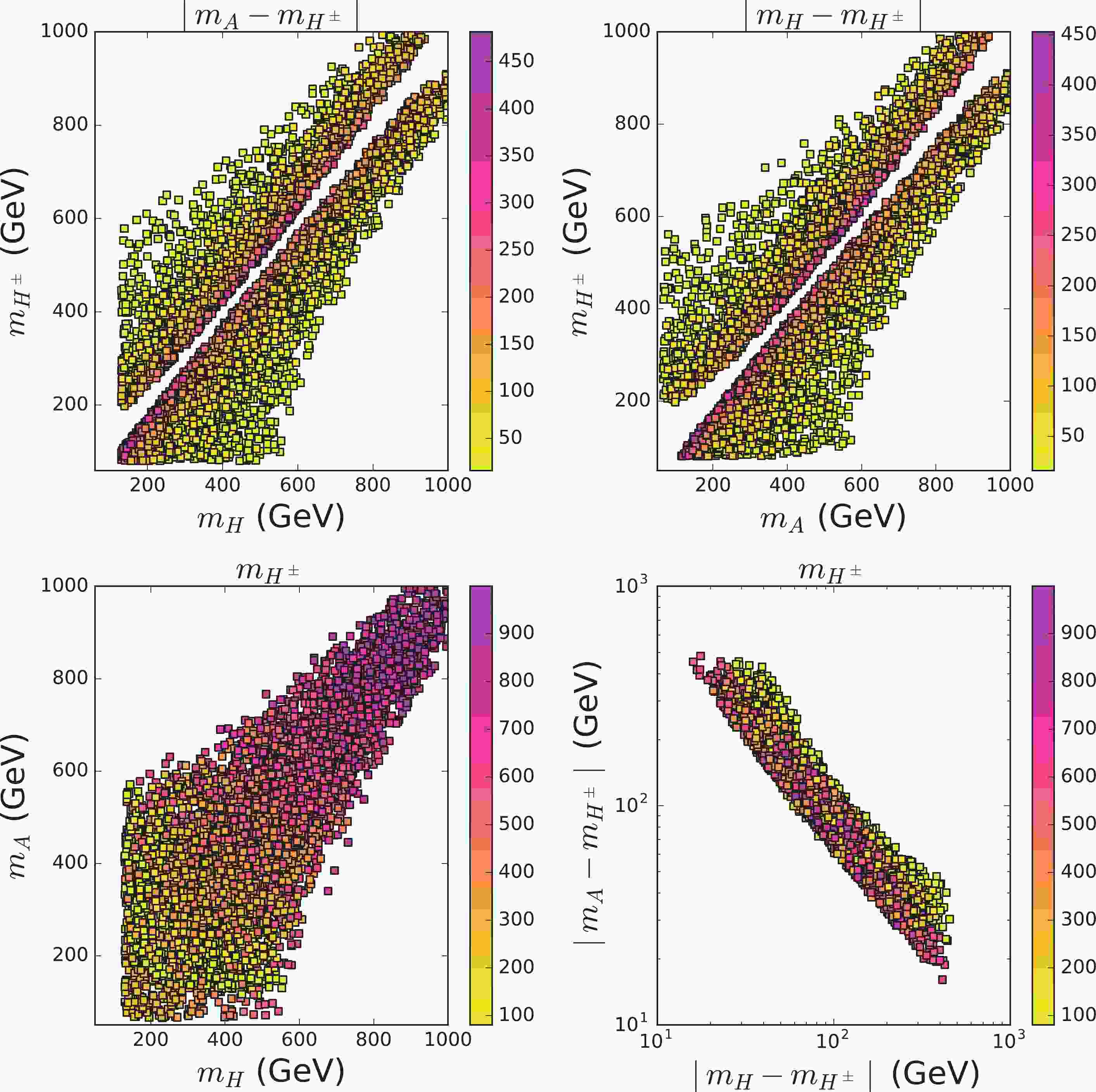
(12) In Figs. 1 and 2, we show samples explaining the CDF W-boson mass measurement within a
$ 2\sigma $ range while satisfying the constraints on the oblique parameters and theory. From Figs. 1 and 2, we see that H or A is disfavored to exactly degenerate in mass with$ H^\pm $ ; however, their masses are allowed to be degenerate. The mass splitting between$ H^\pm $ and$ H/A $ imposes upper and lower bounds and is required to be larger than approximately 10 GeV. When$ m_H $ or$ m_A $ is close to$ m_{H^\pm} $ , the other is allowed to have sizable deviation from$ m_{H^\pm} $ .$ m_{H^\pm} $ and$ m_{A} $ are favored to be smaller than 650 GeV for$ m_H<120 $ GeV (see Fig. 2) and allowed to have larger values with increasing$ m_H $ (see Fig. 1).
Figure 1. (color online) For
$ m_H> $ 130 GeV, samples explaining the CDF II results of W-mass within a$ 2\sigma $ range while satisfying the constraints of the oblique parameters and theoretical constraints. The varying colors in each panel indicate the values of$ \mid m_A-m_{H^\pm}\mid $ ,$ \mid m_H-m_{H^\pm}\mid $ , and$ m_{H^\pm} $ .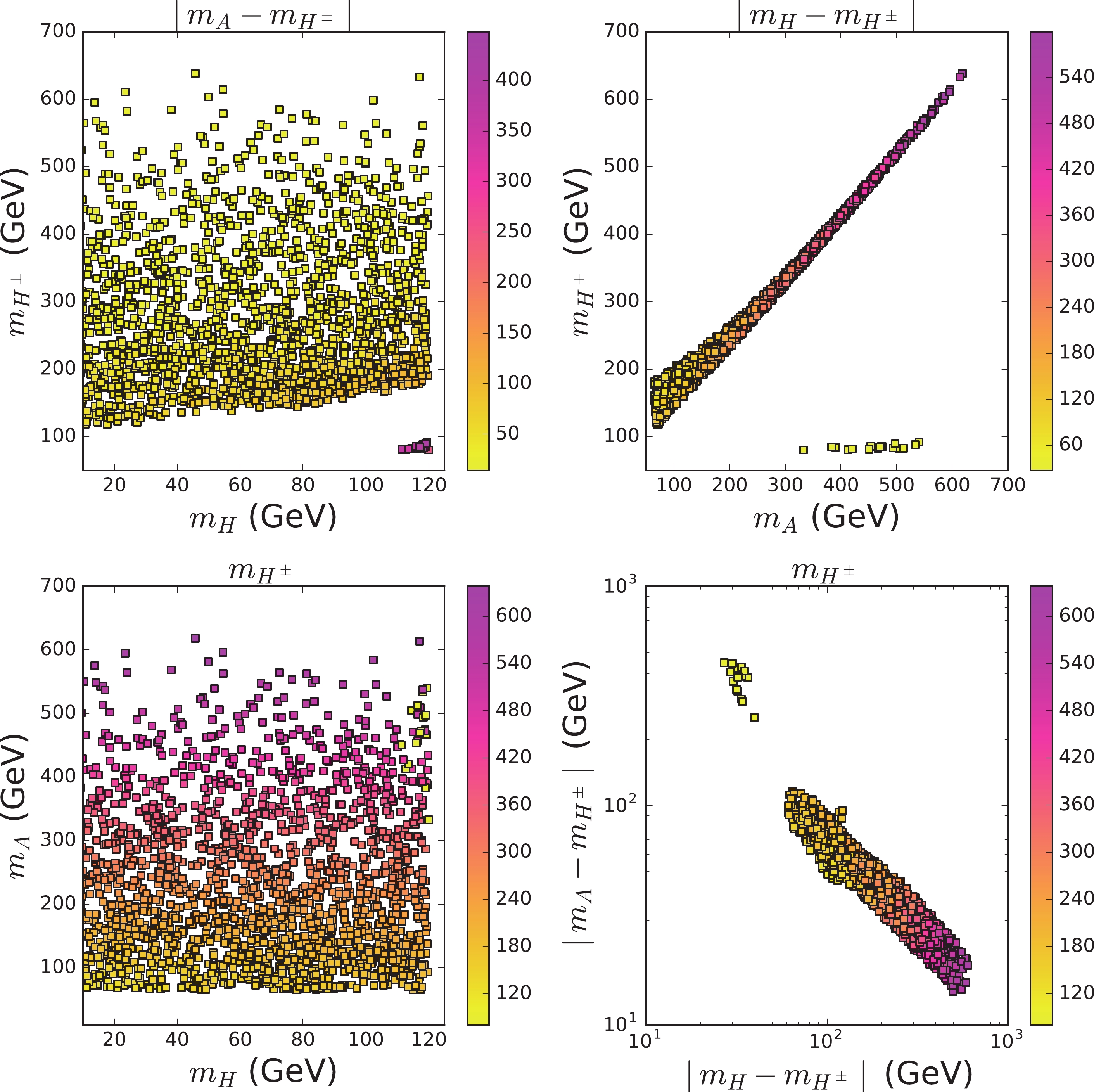
Figure 2. (color online) Same as Fig. 1 but for
$ m_H< $ 120 GeV.Now, we analyze the reason. In the model, the correction to the T parameter is expressed as
$ \begin{aligned}[b] T= &\; \frac{1}{16\pi M_W^2s_W^2}\, \Biggl\{ \biggl[ \mathcal{F}(M_{H^\pm}^2,M_H^2) \\&- \mathcal{F}(M_H^2,M_A^2) + \mathcal{F}(M_{H^\pm}^2,M_A^2) ] \; \Biggr\}\, , \end{aligned} $

(13) where the
$ \mathcal{F} $ function is [66–68]$ \begin{equation} \mathcal{F}(m_1^2,m_2^2) = \frac{1}{2}\, (m_1^2+m_2^2)-\frac{m_1^2m_2^2}{m_1^2-m_2^2}\; \log{\left(\frac{m_1^2}{m_2^2}\right)}\, . \end{equation} $

(14) The function
$ \dfrac{\mathcal{F}(m_1^2,m_2^2)}{m_W^2} $ and factor$ \dfrac{1}{16\pi s_W^2} $ in the T parameter are usually larger than those of the S and U parameters. Therefore, in general, one expects T to be dominant in oblique corrections. Detailed discussions can be found in Ref. [69]. The expressions in Eqs. (13) and (14) show that the T parameter is sensitive to the mass splittings among$ H,\; A $ , and$ H^{\pm} $ . The T parameter will be zero for$ m_H = m_{H^\pm} $ or$ m_A = m_{H^\pm} $ but takes a non-zero value for$ m_A = m_{H} $ . Therefore, the corrections of the model to the oblique parameters tend to decrease as either$ m_H $ and$ m_{A} $ approaches$ m_{H^\pm} $ . However, to accommodate the W-mass reported by the CDF II collaboration, the model must produce an appropriate value of T, which excludes$ m_H = m_{H^\pm} $ or$ m_A = m_{H^\pm} $ . -
The model gives additional corrections to the muon
$ g-2 $ anomaly ($ \Delta a_{\mu} $ ) via one-loop diagrams involving the μ-τ LFV couplings of H and A [44–46].$ \begin{eqnarray} \Delta a_{\mu} = \frac{m_\mu m_\tau \rho^2}{8\pi^2} \left[\frac{ \left(\log\dfrac{m_H^2}{m_\tau^2} - \dfrac{3}{2}\right)}{m_H^2} -\frac{\log\left( \dfrac{m_A^2}{m_\tau^2}-\dfrac{3}{2}\right)}{m_A^2} \right]. \end{eqnarray} $

(15) Here, we find that
$ \Delta a_{\mu}>0 $ for$ m_A>m_H $ .Because the extra Higgs bosons have μ-τ LFV interactions, the model can affect lepton flavor universality (LFU) in τ lepton decays. The HFAG collaboration tested LFU from the ratios of the partial widths of a heavier lepton. They obtained [70]
$ \begin{aligned}[b] \left( \frac{g_\tau}{g_\mu}\right) =& 1.0011\pm0.0015, \quad\left( \frac{g_\tau}{g_e}\right) = 1.0029\pm0.0015,\\ \left( \frac{g_\mu}{g_e}\right) =& 1.0018\pm0.0014, \end{aligned} $

(16) using pure leptonic processes, namely,
$ \begin{align} \left( \frac{g_\tau}{g_\mu}\right)^2 & \equiv \frac{ \overline{\Gamma}(\tau\to e \nu \overline{\nu})}{\overline{\Gamma}(\mu \to e \nu \overline{\nu})}, \end{align} $

(17) $ \begin{align} \left( \frac{g_\tau}{g_e}\right)^2 & \equiv \frac{ \overline{\Gamma}(\tau\to \mu \nu \overline{\nu})}{\overline{\Gamma}(\mu \to e \nu \overline{\nu})}, \end{align} $

(18) $ \begin{align} \left( \frac{g_\mu}{g_e}\right)^2 &\equiv \frac{ \overline{\Gamma}(\tau\to \mu \nu \overline{\nu})}{\overline{\Gamma}(\tau \to e \nu \overline{\nu})}, \end{align} $

(19) with
$ \overline{\Gamma} $ representing the partial width, which is normalized by the corresponding SM value.$ g_{e\; (\mu,\tau)} $ denote the effective couplings between e$ (\mu,\tau) $ and$ \nu_e $ $ (\nu_\mu,\nu_\tau) $ . With the two semi-hadronic processes,$ \begin{align} \left( \frac{g_\tau}{g_\mu}\right)_h^2 & \equiv \frac{ {\rm{Br}} (\tau\to h \nu) }{{\rm{Br}} (h\to \mu \overline{\nu})} \frac{2m_hm_\mu^2\tau_h}{(1+\delta_h) m_\tau^2 \tau_\tau} \left( \frac{1-m_\mu^2/m_h^2}{1-m_h^2/m_\tau^2} \right)^2, \end{align} $

(20) where h indicates π or K, they measure
$ \begin{align} \left( \frac{g_\tau}{g_\mu}\right)_\pi = 0.9963\pm0.0027, \; \; \; \; \; \left( \frac{g_\tau}{g_\mu}\right)_K = 0.9858\pm0.0071. \end{align} $

(21) The statistical correlation matrix for the five fitted coupling ratios is
$\left[\begin{array}{ccccc} 1 & 53 \% & -49 \% & 24 \% & 12 \% \\ 53 \% & 1 & 48 \% & 26 \% & 10 \% \\ -49 \% & 48 \% & 1 & 2 \% & -2 \% \\ 24 \% & 26 \% & 2 \% & 1 & 5 \% \\ 12 \% & 10 \% & -2 \% & 5 \% & 1 \end{array}\right].$

(22) In this model, we can calculate
$ \begin{aligned}[b] &\bar{\Gamma}(\tau\to \mu \nu\bar{\nu}) = (1+\delta_{\rm{loop}}^\tau)^2\; (1+\delta_{\rm{loop}}^\mu)^2+\delta_{\rm{tree}},\\ &\bar{\Gamma}(\tau\to e \nu\bar{\nu}) = (1+\delta_{\rm{loop}}^\tau)^2,\\ &\bar{\Gamma}(\mu\to e \nu\bar{\nu}) = (1+\delta_{\rm{loop}}^\mu)^2. \end{aligned} $

(23) The tree-level correction
$ \delta_{\rm{tree}} $ is from the contribution of$ H^\pm $ to$ \tau\to \mu\nu\overline{\nu} $ ,$ \begin{equation} \delta_{\rm{tree}} = 4\frac{m_W^4\rho^4}{g^4 m_{H^{\pm}}^4}, \end{equation} $

(24) which can give a positive correction.
$ \delta_{\rm{loop}}^\mu $ and$ \delta_{\rm{loop}}^\tau $ are the corrections to the vertices$ W\bar{\nu_{\mu}}\mu $ and$ W\bar{\nu_{\tau}}\tau $ from one-loop diagrams containing A, H, and$ H^\pm $ . Because we assume$ \rho_{\mu\tau} = \rho_{\tau\mu} $ in the lepton Yukawa matrix, the two corrections are identical [53, 71, 72].$ \begin{equation} \delta_{\rm{loop}}^\tau = \delta_{\rm{loop}}^\mu = {1 \over 16 \pi^2} {\rho^2} \left[1 + {1\over4} \left( H(x_A) + H(x_H) \right) \right]\,, \end{equation} $

(25) where
$ H(x_\phi) \equiv \ln(x_\phi) (1+x_\phi)/(1-x_\phi) $ with$ x_\phi = m_\phi^2/m_{H^{\pm}}^2 $ . Meanwhile, for the semi-hadronic processes, we have$ \begin{equation} \left( g_\tau \over g_\mu \right) = \left( g_\tau \over g_\mu \right)_K = \left( g_\tau \over g_\mu \right)_\pi. \end{equation} $

(26) In our study, we perform a global fit to the predictions of these five ratios. Note that there is a vanishing eigenvalue in the covariance matrix constructed from Eqs. (16), (21), and (22), and therefore such a degree of freedom is removed. Using the remaining four degrees of freedom, the
$ 2\sigma $ confidence level region is obtained by adopting a limit of$ \chi^2_\tau<9.72 $ . Thus, the surviving samples are considerably more consistent with the experimental results than that of the SM, which has a$ \chi^2_\tau $ of$ 12.25 $ . Furthermore, the model can affect LFU in Z-boson decays [73], and the constraints from Z-boson decays are generally weaker than those from τ decays.In the model, the fields H, A, and
$ H^{\pm} $ have no couplings to quarks; therefore, they are produced at the LHC mainly via electroweak processes,$ pp\to W^{\pm *} \to H^\pm A/H $ ,$ pp\to Z^* \to HA $ , and$ pp\to Z^*/\gamma^* \to H^+H^- $ . The final state signal mainly includes multi-leptons, and therefore multi-lepton event searches at the LHC can impose stringent constraints that require$ m_H $ to be larger than 560 GeV [55]. Moreover, a very light H may escape the constraints of direct searches at the LHC [56]. In this case, the explanation of the muon$ g-2 $ anomaly requires a small ρ, which leads to the contributions of the model to τ decays being too small to explain the data of LFU in the τ decays. Therefore, in this study, we discuss the scenario for$ m_H>560 $ GeV. In addition, to respect perturbativity, we choose the Yukawa coupling parameter$ \rho<1 $ .At tree level, the 125 GeV Higgs has the same couplings to SM particles as in the SM. The
$ h\to \gamma\gamma $ decay will be corrected by the one-loop diagram of the charged Higgs [74]. We consider the bound of the diphoton signal strength [2] to be$ \begin{equation} \mu_{\gamma\gamma} = 1.11^{+0.1}_{-0.09}. \end{equation} $

(27) In Fig. 3, we project the surviving samples explaining the muon
$ g-2 $ anomaly and LFU in τ-decays within$ 2\sigma $ ranges, satisfying other relevant constraints from theory, the oblique parameters, the CDF II W-mass, and the diphoton signal data of the 125 GeV Higgs. Eq. (15) shows that H and A give positive and negative contributions to muon$ g-2 $ , respectively, and their contributions are suppressed by their masses. Therefore, the explanation of muon$ g-2 $ requires$ m_A > m_H $ and ρ to increase with increasing$ m_H $ and decreasing$ (m_A-m_H) $ (see the upper-left panel).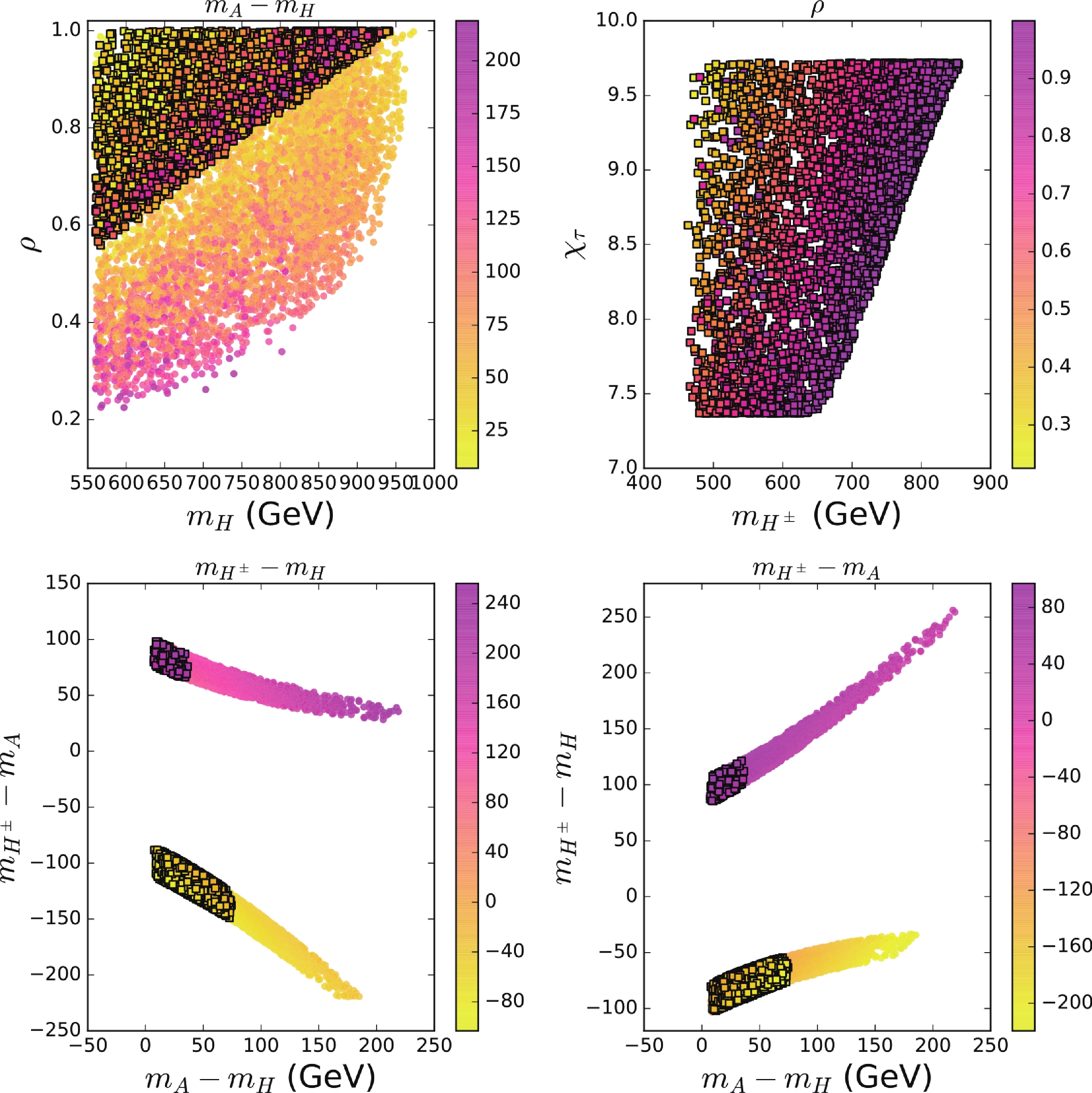
Figure 3. (color online) Bullets explain muon
$ g-2 $ within a$ 2\sigma $ range, whereas the squares explain muon$ g-2 $ and τ-decays within$ 2\sigma $ ranges while satisfying the constraints of Z-decays. Other relevant constraints from theory, the oblique parameters, the CDF II W-mass, and the diphoton signal data of the 125 GeV Higgs are also satisfied. The varying colors in each panel indicate the values of$ m_A-m_{H} $ , ρ,$ m_{H^\pm}-m_H $ , and$ m_{H^\pm}-m_A $ .The ratio
$ \left( {g_\tau} / {g_e }\right) $ in τ decays has a deviation of approximately$ 2\sigma $ from the SM. Therefore, enhancing$ \Gamma(\tau\to \mu \nu\bar{\nu}) $ may give a better fit to the data of LFU in the τ decays. The decay$ \tau\to \mu\nu\nu $ obtains a positive correction from the$ \delta_{\rm{tree}} $ term of Eq. (23). Such a term is from the tree-level diagram mediated by the charged Higgs and proportional to$ \rho^4/m^2_{H^\pm} $ . Therefore, the upper-right panel of Fig. 3 shows that the value of$ \chi_\tau^2 $ tends to increase with increasing$ m_{H^\pm} $ and decreasing ρ. In addition, because of the constraints of the oblique parameters and W-boson mass, the upper-left panel of Fig. 1 shows that$ m_{H^\pm} $ tends to increase with$ m_H $ , especially for large$ m_H $ , which implies that the value of$ \chi_\tau^2 $ increases with increasing$ m_H $ . Therefore, the upper-left panel of Fig. 3 shows that a simultaneous explanation of muon$ g-2 $ and LFU in τ decays favors a large ρ that increases with$ m_H $ .From the lower panel of Fig. 3, we see that the mass splittings among H, A, and
$ H^\pm $ are stringently constrained in the region simultaneously explaining W-mass, muon$ g-2 $ , and LFU in τ decays, that is, 1$ <m_A-m_H< $ 75 GeV, 65$ <m_{H^\pm}-m_A< $ 100 GeV, and 85$ <m_{H^\pm}-m_H< $ 125 GeV (–150$ <m_{H^\pm}-m_A< $ –85 GeV, and –105$ <m_{H^\pm}-m_H< $ –55 GeV).In the model, pair production of extra Higgs bosons via electroweak processes at the LHC leads to detectable multi-lepton signals containing μ and τ. The current lower bound of 560 GeV on
$ m_H $ is mainly obtained from the CMS search for the electroweak production of charginos and neutralinos in multilepton final states [75]. By normalizing the number of background and signal events, the lower bound on$ m_H $ can be increased to 700 GeV for 300 fb$ ^{-1} $ of integrated luminosity data. Adopting the same procedure, we estimate that more than 3000 fb$ ^{-1} $ of integrated luminosity data is required to cover the entire surviving parameter, namely,$ m_H<950 $ GeV. However, this CMS search was originally designed to search for SUSY particles. A dedicated study focusing on$ \mu\tau $ final states and improving signal regions for the high mass region can greatly reduce the required integrated luminosity to an acceptable level, which is beyond the scope of this paper. -
We examine the CDF II W-boson mass and FNAL muon
$ g-2 $ in the 2HDM in which the extra Higgs doublet has μ-τ LFV interactions. Imposing theoretical constraints, we find that the CDF II W-boson mass disfavors H or A degenerating in mass with$ H^\pm $ , and the mass splitting between$ H^\pm $ and$ H/A $ is favored to be larger than 10 GeV.$ m_{H^\pm} $ and$ m_{A} $ are favored to be smaller than 650 GeV for$ m_H<120 $ GeV and allowed to have larger values with increasing$ m_H $ . Considering other relevant experimental constraints, we find that the mass splittings among$ H,\; A $ , and$ H^\pm $ are stringently restricted in the parameter space, which can simultaneously explain the CDF II W-mass, the FNAL muon$ g-2 $ , and LFU data in τ decays. -
We thank Lei Wu for helpful discussions.
-
The quartic couplings of the scalar potential in Eq. (3) cannot be too large individually otherwise the theory will no longer be perturbative. Thus, we require
$ \mid\lambda_{1,2,3,4,5}\mid \leq 4\pi. \tag{A1} $

-
Vacuum stability requires the potential to be bound from below and remain positive for arbitrarily large values of the fields. This requirement leads to restrictions on the parameters of the model.
$ \lambda_1 > 0,\;\; \lambda_2 > 0,\;\; \lambda_3 + \sqrt{\lambda_1\lambda_2} > 0, \;\; \lambda_3 + \lambda_4 - \mid\lambda_5\mid +\sqrt{\lambda_1\lambda_2} > 0. \tag{A2} $

-
The amplitudes for the scalar-scalar scattering
$ s_1 s_2 \to s_3 s_4 $ at high energies respect unitarity, which leads to the following bounds on the parameters of the model [76, 77]:$ |a_{\pm}|, |b_\pm|, |c_\pm|, |{\tt e}_\pm|, |{\tt f}_\pm|, |{\tt g}_\pm| \,\le\, 8\pi \, , \tag{A3}$

with
$ a_\pm^{} = \tfrac{3}{2}(\lambda_1+\lambda_2) \pm \sqrt{\tfrac{9}{4}(\lambda_1-\lambda_2)^2+(2\lambda_3+\lambda_4)^2} \,, \tag{A4} $

$ b_\pm^{} = \tfrac{1}{2}(\lambda_1+\lambda_2) \pm \sqrt{\tfrac{1}{4}(\lambda_1-\lambda_2)^2+\lambda_4^2} \,, \tag{A5} $

$ \begin{eqnarray} c_\pm^{} \,& = &\, \tfrac{1}{2}(\lambda_1+\lambda_2) \pm \sqrt{\tfrac{1}{4}(\lambda_1-\lambda_2)^2+\lambda_5^2} \,, \end{eqnarray} \tag{A6}$

$ \begin{eqnarray} {\tt e}_\pm^{} & = & \lambda_3^{} + 2 \lambda_4^{} \pm 3 \lambda_5^{} \,, \end{eqnarray}\tag{A7} $

$ \begin{eqnarray} {\tt f}_\pm^{} \,& = &\, \lambda_3^{} \pm \lambda_4^{} \,, \end{eqnarray} \tag{A8}$

$ \begin{eqnarray} {\tt g}_\pm \,& = &\, \lambda_3^{} \pm \lambda_5^{} \,. \end{eqnarray} \tag{A9}$

Joint explanation of W-mass and muon g–2 in the 2HDM
- Received Date: 2022-05-19
- Available Online: 2022-10-15
Abstract: Because both W-mass and muon


 DownLoad: