Discovery of new characterizations of parameter distributions in a semi- empirical mass model: an investigation by dividing an overdetermined system into numerous balanced subsystems

Nuclei communicate with us through various observables [1]; however, in principle, no measurement or calculation can reveal the ultimate truth behind them. Besides experimental uncertainties, the demand for theoretical error bars on the predicted physical-quantities of models is increasing, especially since the sentiment was articulated by the editors of Physical Review A in 2011 [2]. Indeed, a theoretically good model should possess a strong predictive power as well as a strong descriptive (or explanatory) power.

To determine the predictive and descriptive power of a model, one must evaluate not only the difference between the calculated and experimental values of the concerned observables but also whether this difference is sufficiently significant. For a relatively good model, a small difference is certainly expected, with a value considered insignificant according to the given significance level. With the aid of statistical theory and ignoring experimental errors, one can similarly conduct significance testing on the difference between theory (with uncertainty) and experiment for an individual nucleus. For instance, suppose that the theoretical prediction has a Gaussian-distributed shape with mean μ and standard deviation σ (other distribution assumptions are similar). After defining a variable $ z=(\Delta-\Delta_\mu)/\sigma $, where $ \Delta_\mu $ is the difference between the predicted mean value μ and experimental data, and Δ denotes the difference between the calculated and experimental values, one can obtain a $ K_\alpha $ value (α is a given significance level) based on the probability condition $P(\Delta \geq K_\alpha \sigma) = 1-2\int_0^{K_\alpha} \frac{1}{\sqrt{2\pi}}{\rm e}^{-z^2/2} {\rm d}z =\alpha$. If the value K($ \equiv \Delta_{\mu}/\sigma $) is smaller than $ K_\alpha $, the difference is considered insignificant, indicating an acceptable prediction. However, for $ K \geq K_\alpha $, the difference is significant, and the prediction will be considered poor from the statistical perspective.

As mentioned above, the parameter uncertainties and their propagation in a theoretical model are important for evaluating its descriptive and predictive power. However, estimating model parameters and their respective uncertainties is fraught with difficulty. In general, the $ \chi^2 $ or basic bootstrap method greatly underestimates the uncertainty on the parameter distribution in many circumstances [3]. In addition, parametric correlations strongly affect uncertainty propagation [4]. We consider the phenomenological Bethe-Weizsäcker formula and its variant as a testing ground for estimating model parameters and their uncertainties, correlations, and propagation [5]. Note that the importance of nuclear masses (or binding energies) is widely stressed in literature (e.g., see Refs. [3, 6] and references therein).

To our knowledge, the uncertainty on the theoretical prediction of binding energy for an individual nucleus is typically either too small (based on the formula for uncertainty propagation, correlations, and the available uncertainties on model parameters) or too large (without the inclusion of parametric correlations). Such prediction is generally meaningless because the error is too large or the deviation from data is too significant. Therefore, most published studies have not touched upon the so-called predictive power for individual nuclei and have instead illustrated the descriptive accuracy and predictive power of a given mass model using the r.m.s. (root-mean-square) value of the differences between the theoretical and experimental values and the r.m.s. variant [7, 8]. Sobiczewski et al. [8] evaluated the descriptive and predictive power of ten frequently-used mass-models and different nuclear regions.

In this study, we propose a new method in which we split an overdetermined system into numerous balanced subsystems to evaluate the modeling parameters, parameter uncertainties, and uncertainty propagation. Interestingly, it is found that the parameter distribution has a Cauchy (Breit-Wigner or Lorentzian) line shape, which is similar to a Gaussian distribution near the peak, but with flatter curve tails. This line shape is often adopted, e.g., in quantum field theory, as an approximate model of the resonance (unstable particle) propagator [9]. It has also been used in the analysis of the Raman spectra of graphene [10, 11]. In statistics, this distribution can be generated by using the ratio of two independent normal variables. However, it must be stressed that our main aim in this study is to present the Cauchy-type parameter distributions and investigate their correlations and uncertainty propagation. The physics behind such a parameter distribution, e.g., in the semi-empirical mass model, is not our primary concern, but further discussion will be of interest in the future.

This paper is organized as follows. In Sec. II, we specify the related theory used in the present investigation. The results and discussion are presented in Sec. III. Finally, we summarize our study in Sec. IV.

Here, we provide a brief presentation of the investigative procedure used in this study. The selected toy model is the semi-empirical Bethe-Weizsäcker formula [12–16], which parametrizes the binding energy of the nucleus $ (Z,N) $ into the following main terms:

where $ A_i = Z_i + N_i $ is the mass number of the ith nucleus, and the successive terms represent the volume, surface, Coulomb, and symmetry energies, respectively. Through comparison with data, one can evaluate the theoretical modeling and model parameters. Indeed, numerous related studies can be found in literature [6, 16–19].

From Eq. (1), we can see that the deformation, shell, and pairing effects are not included. Of course, there are several phenomenological treatments for each of these. In this study, as mentioned in Refs. [20, 21], we define the microscopic energy to cover such effects, namely,

where $ E_{{\rm{def}}} $, $ E_{{\rm{shell}}} $, and $ E_{{\rm{pair}}} $ denote the deformation, shell, and pairing corrections, respectively. For a nucleus, the equilibrium shape in the ground state is indicated by $ \hat{\beta} $, which can be obtained by a standard potential-energy-surface calculation (e.g., see Refs. [22–25] and references therein). The deformation correction energy is calculated using [26, 27]

where $ B_{s} $ and $ B_{c} $ are functions of the shape of the nucleus only and are equal to 1 when the nucleus is spherical. $ E^{(0)}_{s} $ and $ E^{(0)}_{c} $ refer to the spherical surface energy and spherical Coulomb energy, respectively. The shell and pairing corrections are calculated using the Strutinsky method [28] and Lipkin-Nogami (LN) method [29], respectively.

Naturally, it is expected that if the modeling process includes the microscopic corrections mentioned above, it will be able to better describe or predict the experimental data. Equivalently, if the microscopic part is removed from the experimental data, Eq. (1) can describe the remaining 'macroscopic' part more accurately. Keeping this in mind, we define the theoretically corrected experimental binding energies using the equation below (similar to the definition in Ref. [6]).

where $ (B_{{\rm{Exp}},i}) $ and $ (E_{{\rm{mic}},i}) $ denote the uncorrected experimental binding energy and microscopic energy (defined in Eq. (2)), respectively. The uncorrected experimental nuclear binding energy is obtained from the 2016 atomic mass evaluation (2016AME) [30, 31]. Combining Eq. (1) and the large database $ \{ B_{{\rm{Exp}}}\} $ or $ \{ B^{\prime}_{{\rm{Exp}}}\} $, we can obtain a linear system of equations. There is usually no exact solution to such an overdetermined system. In general, one can search for the solution with the smallest error vector using a vector norm (i.e., a Euclidean norm, Manhattan norm, or Chebyshev norm) to determine the size of the error vector. For instance, the fitting criterion of the Chebyshev norm was adopted in Ref. [32]. In the least squares method frequently used in literature, one searches for the error vector with the smallest L2-norm. That is, this method minimizes the penalty function

Fitting procedures can easily be found from literature [1, 33–35]. For instance, by setting the partial derivatives of $ \chi^{2} $ with respect to the various parameters equal to zero, we can obtain a set of linear equations with four variables $ a_v $, $ a_s $, $ a_c $, and $ a_a $. The system is solved using Gauss's method. With these parameters, we can evaluate and predict the nuclear binding energy of a nucleus and provide the r.m.s. deviation, which is typically used to characterize the goodness-of-fit [6].

The experimental uncertainty on the binding energy is generally small [30, 31], and the numerical uncertainty on a linear and analytical model is negligible [19]. We use two methods to obtain the parameter distributions in Eq. (1). One method, based on general treatments, involves constructing a statistical model for the binding energies B according to the formula below, e.g., cf. Eq. (2) in Ref. [16].

The errors are modeled as an independent standard normal random variable $ \epsilon_i $, scaled by an error factor σ. The Gaussian random numbers are generated using the Box-Muller algorithm [36–40]. If the r.m.s. error is known as $ priori $, the scaling parameter σ can be fixed. For instance, it was noted [19] that the total uncertainties are approximately 0.5 MeV from the fitting procedure in different models, including the finite-range droplet model [21], Lublin-Strasbourg drop model [41], Hartree-Fock-Bogoliubov model [42, 43], and Weizsäker-Skyrme mass model [44, 45]. Otherwise, they can be estimated according to the calculation mention above. For each set of different $ \{\sigma\epsilon_i\} $, we can obtain a set of parameters $ \{a_i\} $ using least-squares fitting. After sufficient Monte Carlo replications [46–48], we can obtain the corresponding parameter distributions.

It must be stressed that another idea for evaluating the parameter uncertainty is to divide the overdetermined system into numerous small balanced subsystems, which can be solved exactly. For instance, if accepting the semi-empirical Bethe-Weizsäcker formula [14–16], as seen in Eq. (1), we can obtain the exact solutions of the model parameters with the help of four solvable equations (equivalently, four binding energies). For the available data n, there are $ C_n^4 $ combinations of equations or binding energies. In principle, we may obtain $ C_n^4 $ sets of model parameters, which can be used for the uncertainty analysis. However, as is known, the 2016AME database includes 2497 available nuclei, which corresponds to $ C_{2497}^4 (\sim 1.616\times 10^{12}) $ combinations, which is too large for practical calculation. Alternatively, we can obtain the corresponding parameter distributions formed by the so-called exact solutions using the Monte-Carlo sampling technique.

The distribution property of model parameters can be analyzed using the maximum likelihood method [49–52], e.g., to extract the location and scale parameters. In this study, the Gaussian- and Cauchy-type probability densities, $f^G(x|\mu,\sigma)=\frac{1}{\sqrt{2\pi\sigma}} {\rm e}^{ \frac{(x-\mu)^{2}}{2\sigma^{2}}}$ and $ f^C(x|\mu,\sigma) =\frac{\sigma/\pi}{(x-\mu)^2+\sigma^2} $, respectively, are used to construct the likelihood function, $ L(\mu,\sigma)=\prod_{i=1}^n f(x_i|\mu,\sigma) $, or the log likelihood function, $\log L(\mu,\sigma)=\displaystyle\sum\nolimits_{i=1}^n \log f(x_i|\mu,\sigma)$, where μ,σ are the position and scale parameters. Maximizing $ \log L(\mu $,$ \sigma) $ with respect to μ and σ will give us the maximum likelihood estimation. For instance, by setting the partial derivatives $ \frac{\partial[\log L(\mu,\sigma)]}{\partial \mu} $ and $ \frac{\partial[\log L(\mu,\sigma)]}{\partial \sigma} $ to zero, we can obtain the location and scale parameters [53] by solving the equation system. Note that, for the Gaussian-distributed case, we can obtain the analytical solutions $ \mu=\bar{x}=\frac{1}{n}\displaystyle\sum\nolimits_{i=1}^n x_i $ and $ \sigma=\sqrt{\frac{1}{n}\displaystyle\sum\nolimits_{i=1}^n (x_i-\bar{x})^2} $. However, for the Cauchy distribution, we must solve the non-linear likelihood equations

A Newton iteration method [54–56] is used to find the solutions. In addition, to evaluate the existing correlations between model parameters, we can also establish the Pearson product-moment correlation coefficient [57] as $ c_{p_i,p_j}={\rm{cov}}(p_{i}, p_{j})/(\sigma_{p_{i}}\sigma_{p_{j}}) $, where $ \sigma_p $ and $ {\rm{cov}}(p_{i}, p_{j}) $ are the variance and covariance, respectively. The uncertainty on the theoretical prediction is strongly affected by parameter correlations. As shown by Eq. (1), the propagating uncertainty on the predicted binding energy can be evaluated if a suitable distribution is obtained, e.g., via calculation using numerous sets of model parameters. Moreover, for Gaussian-distributed parameters, it can be analytically calculated using [58]

Once we know that the BW formula, cf. Eq. (1), can calculate the binding energy for a given nucleus (Z, N), a set of exact model-parameters can be obtained by solving the linear system formed by four similar equations. During the process of solving numerous systems of linear equations, we ignore the singular cases (e.g., $ N=Z $), whose percentage rates are very low. In principle, the following treatments are standard, including the Monte Carlo technique, fitting procedure, uncertainty and correlation analysis. In this section, we present our results and brief discussions.

In this study, our adopted database includes 578 available even-even nuclei from the mass table AME2016 [31]. To analytically calculate the four model parameters as shown in Eq. (1), we must arbitrarily select four nuclear masses (binding energies); their combinations will reach $C_{578}^4 \sim 4.602\times 10^9$, which is still a large number. Alternatively, Monte Carlo sampling will help perform this investigation instead of the calculations across the entire data space. At each sample point ($B_{{\rm Exp}, i}$, $B_{{\rm Exp}, j}$, $B_{{\rm Exp}, k}$, and $B_{{\rm Exp}, l}$) or ($B^{\prime}_{{\rm Exp}, i}$, $B^{\prime}_{{\rm Exp}, j}$, $B^{\prime}_{{\rm Exp}, k}$, and $B^{\prime}_{{\rm Exp}, l}$), the system of linear equations can easily be solved using, e.g., the Gaussian elimination method, inverse matrix method, or Cramer's rule. Here, $ 10^5 $ random samples generated via Monte Carlo simulation are used, with approximately $ \frac{1}{4.602\times 10^4} $ of the above combinations (low repetition rate can also be assured). Figure 1 illustrates the quality of Monte Carlo sampling for the 578 available even-even nuclei mentioned above. The number of times each nucleus is used is presented in the $ Z-N $ map, indicating the random and uniform properties. It should be noted that each sample point involves four nuclei. From Fig. 1, we can see that a random number from 1 to 578 coded for each available nucleus is uniform to a large extent. The statistical distribution of the percentage rates is Gaussian, as shown in inset (b).

Figure 1.  (color online) Distribution of $ 10^5 $ four-nucleus samples from 578 available even-even nuclei with $ Z \geq 20 $ in the mass table AME2016 [31]. Legends with different colors denote different sampling number intervals, and the number in the first and second brackets are the nucleus number between the corresponding interval and the percentage rate, respectively. Inset (a) shows the uniform property of Monte Carlo sampling for the 578 coded nuclei. The fluctuation of Monte Carlo sampling near the average value is shown in inset (b) along with the Gaussian fit (solid line).

To extract the theoretically-corrected experimental binding energies, we calculate the microscopic energies of the 578 even-even nuclei using the potential-energy-surface method [22], as shown in Fig. 2(similarly, we recently performed a global calculation with the inclusion of the Coriolis effect [59]). From Eq. (1), we can easily notice that the nuclear binding energy of a given nucleus (Z, N, or A) depends on the model parameters $ \theta \equiv (a_v, a_s, a_c, a_a) $. When comparing this theoretical result with the experimental binding energy $B_{\rm Exp}$, these parameters should be pairing-, shell-, and deformation-dependent because the expression in Eq. (1) does not include such terms. Of course, when considering the theoretically-corrected experimental binding energy $B^{\prime}_{\rm Exp}$ (equivalently, improving the model to include the so-called microscopic energy defined above), these model parameters can be assumed to be pairing-, shell-, and deformation-independent, at least to a large extent. The uncertainties on these model parameters are expected to decrease by improving the modeling.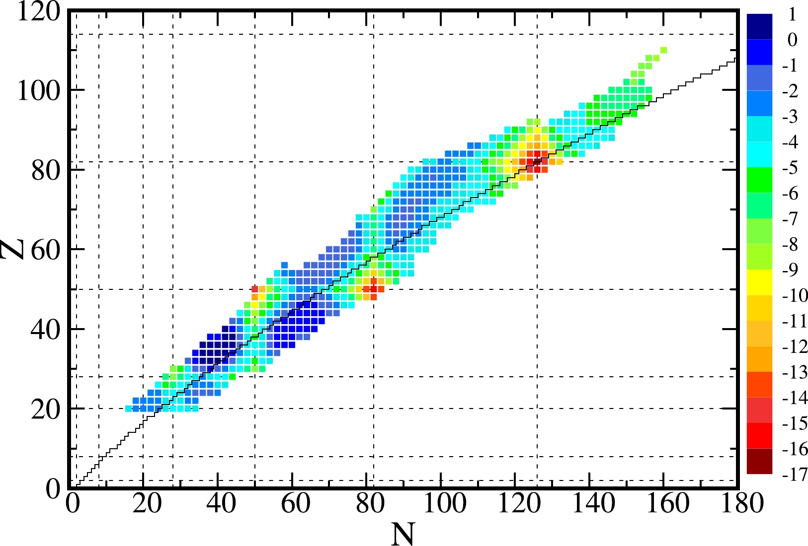

Figure 2.  (color online) Systematic calculations of the microscopic energies (in units of MeV) defined in Eq. (2) for 578 even-even nuclei with $ Z \geq 20 $ using the potential-energy-surface method [22]. The black line represents the β-stability line, and the dash lines correspond to magic numbers, which are simply there to guide the eyes.

Figure 3 shows the distributions of the model parameters formed by the exact solutions of numerous balanced systems based on the uncorrected [left: (a), (b), (c), and (d)] and theoretically-corrected [right: (e), (f), (g), and (h)] experimental data. The distribution test is simultaneously presented on the right of the corresponding parameter distribution, e.g., (a$ ^\prime $) corresponds to (a). First, we transform the general Cauchy distribution into a standard form $ P(z)=\frac{1}{\pi (1+z^2)} $ by setting $ z =\frac{x-\mu}{\sigma} $, where x, μ, and σ are the variable (e.g., the parameter $ a_v $), location, and scale parameters, respectively. Integrating the Cauchy distribution function and setting the upper and lower limits of integration as $ +k\sigma $ and $ -k\sigma $, for $ k\geq 0 $, we can obtain

Figure 3.  (color online) Left: Distributions of model parameters $ a_v $ (a), $ a_s $ (b), $ a_c $ (c), and $ a_a $ (d) obtained based on the uncorrected experimental data. The solid curves denote the Cauchy-distributed curves with position (which is selected as the origin of the horizontal coordinate) and scale parameters obtained using the maximum likelihood estimation. Note that the left and right numbers of the corresponding distribution are its position and scale parameters, respectively, in units of MeV. The relatively small figures (a$ ^\prime $), (b$ ^\prime $), (c$ ^\prime $), and (d$ ^\prime $) on the right side of these distributions show the confidence levels calculated using the parameter histograms (symbols) and standard Cauchy distribution (solid curves). Right: same as the left but based on the theoretically-corrected experimental data. See text for further details.

For each k, we can obtain theoretical integration for the Cauchy distribution. By comparison with the value obtained from the practical parameter distributions, we can test the parameter distribution. Fig. 3 illustrates the good agreement between the corresponding distribution and the Cauchy assumption.

For comparison and to cross-check our results, Table 1 presents several sets of model parameters fitted using different methods and based on different data. The uncorrected and theoretically-corrected experimental data are adopted in the first (I and II) and last (III and IV) two cases, respectively. In cases I and III, the parameter and its uncertainty are evaluated using the least-squares solutions of the overdetermined system. In the other two cases (II and IV), these are given by the exact solutions of the numerous balanced subsystems with the aid of the maximum likelihood method. For comparison purposes, we give the full width at half maximum (FWHM) of the distributions, which are $ 2\sqrt{2\ln2}\sigma $ ($ \sim 2.355\sigma $) and 2σ for the Gaussian and Cauchy distributions, respectively. Note that σ is the scale parameter of the corresponding distribution. The parameter FWHM can be used to describe the width of any ''bump'' (distribution). By comparing the different fitting results, we find that the differences between corresponding position parameters are small; however, those of scale parameters are relatively large. The uncertainties obtained using the maximum likelihood method based on the so-called exact solutions are greater than those of the traditional least-squares treatment. Indeed, the parameter distributions formed by the exact solutions of model parameters mainly originate from the uncertainty on the theoretical modeling (assuming that the statistical and numerical uncertainties, which are usually very small, can be neglected). We can imagine that the parameter set will only be obtained if the BW formula is accurate for each nucleus. It may be reasonable to believe that the present uncertainties, e.g., in cases II and IV, contain systematic errors, which are generally difficult to determine. Their extraction will be of interest in future studies by, e.g., using or developing the uncertainty decomposition method [19]. From Table 1, we also can find that the improvement in the theoretical modeling (e.g., using the theoretically-corrected data) decreases the uncertainties on the model parameters and the r.m.s value of the binding energy, as expected. Based on the even-even nuclei of the 2003 mass table, Bertsch et al. [53] found a similar r.m.s. deviation of $ \sim 3 $ MeV, and using various Skyrme parametrizations, r.m.s. residuals were obtained in the range of $ 1.5-1.7 $ MeV [53].

	I	II	III	IV
$ a_{v} $	15.54447	15.34563	15.72056	15.68743
	0.44898	2.56674	0.22999	1.18858
$ a_{s} $	16.83831	16.36766	17.54223	17.52071
	1.43281	8.01136	0.73389	3.79060
$ a_{c} $	0.70507	0.68889	0.71553	0.71152
	0.02965	0.17382	0.01519	0.07918
$ a_{a} $	23.20229	22.67591	23.87398	23.73727
	1.08707	6.56428	0.55696	3.01518
$ \sigma_{{\rm{r.m.s.}}} $	3.0224	3.4842	1.5491	1.6955

Table 1.  Four sets of model parameters of the BW formula, refitted to 578 even-even nuclei ($ Z\geq 20 $) from the mass table AME2016 [31]. The value in italics below the model parameter denotes the FWHM of its distribution. The last entry gives the corresponding r.m.s. residuals. All energies are in units of MeV. See text for further details

Similar to the two cases in Fig. 3, Fig. 4 illustrates their two-dimensional scatter plots, which can be used to observe the relationships between the model parameters $ a_{v} $, $ a_{s} $, $ a_{c} $, and $ a_{a} $, along with their corresponding correlation coefficients. For simplicity and clarity, we use the dimensionless variables $ \{x_i \} $, which are defined as $ x_i\equiv \frac{p_i-\mu_i}{\sigma_i} $, where $ p_i $, $ \mu_i $, and $ \sigma_i $ are the variable (e.g., the parameter $ a_v $), position, and scale parameters, respectively. In such an operation, the Cauchy distribution is transferred into the standard form. In principle, the expected value and variance cannot be defined for the Cauchy distribution, which has no moment generating function owing to its heavy tails. However, we still can crudely evaluate the correlation property based on the definition of the Pearson coefficient [57] and scatter data. As shown in this figure, in both the left and the right cases, strong correlations almost appear between any two model parameters, agreeing with previous publications. However, the correlation coefficients are slightly different. Spindled and dumbbell shaped distributions are noticed. The improvement in the modeling does not obviously decrease the parameter correlations, though the correlation coefficients shrink slightly.

Figure 4.  (color online) Left: Two-dimensional scatter plots used to observe relationships between two dimensionless variables $ \{x_i \} $, corresponding to the model parameters $ a_{v} $, $ a_{s} $, $ a_{c} $, and $ a_{a} $, along with the corresponding correlation coefficients. Note that the model parameters are obtained based on the uncorrected experimental data at this moment. Right: similar to the left, but the model parameters are obtained based on the theoretically-corrected experimental data. See text for details.

Based on the 10$ ^5 $ sets of model parameters, which automatically include the correlated effects, we can obtain the distribution of the calculated binding energy for each nucleus (equivalently, the propagation uncertainty can be obtained and analyzed). As an example, Fig. 3 shows the propagation uncertainties on the model parameters for the nucleus $ ^{208} $Pb. These distributions have asymmetric shapes and heavy tails, similar to the cases in Refs. [10, 11]. We arbitrarily select two-Cauchy-type distributions to fit the left and right parts of this peak (the fitted location and scale parameters are shown in Fig. 5). As is known, for a symmetric Cauchy distribution with a location parameter μ and scale parameter σ, its FWHM is $ 2\sigma $. Here, as shown in Fig. 5, we give the FWHM values of the asymmetric peaks using $ \sigma_L+\sigma_R $, which are 9.39782 MeV and 3.38051 MeV in (a) and (b), respectively. The deviations $ |\Delta B| $ from $B_{\rm Exp}$ (1636.430 MeV [31]) are 11.920 MeV (approximately 1.27 FWHM) and 0.050 MeV (approximately 0.015 FWHM) in Fig. 5(a) and Fig. 5(b), respectively. Note that in both cases, the deviations are not significant. With improved modeling, both the uncertainty and deviation decrease, and the difference is not significant, indicating a relatively good predictive power.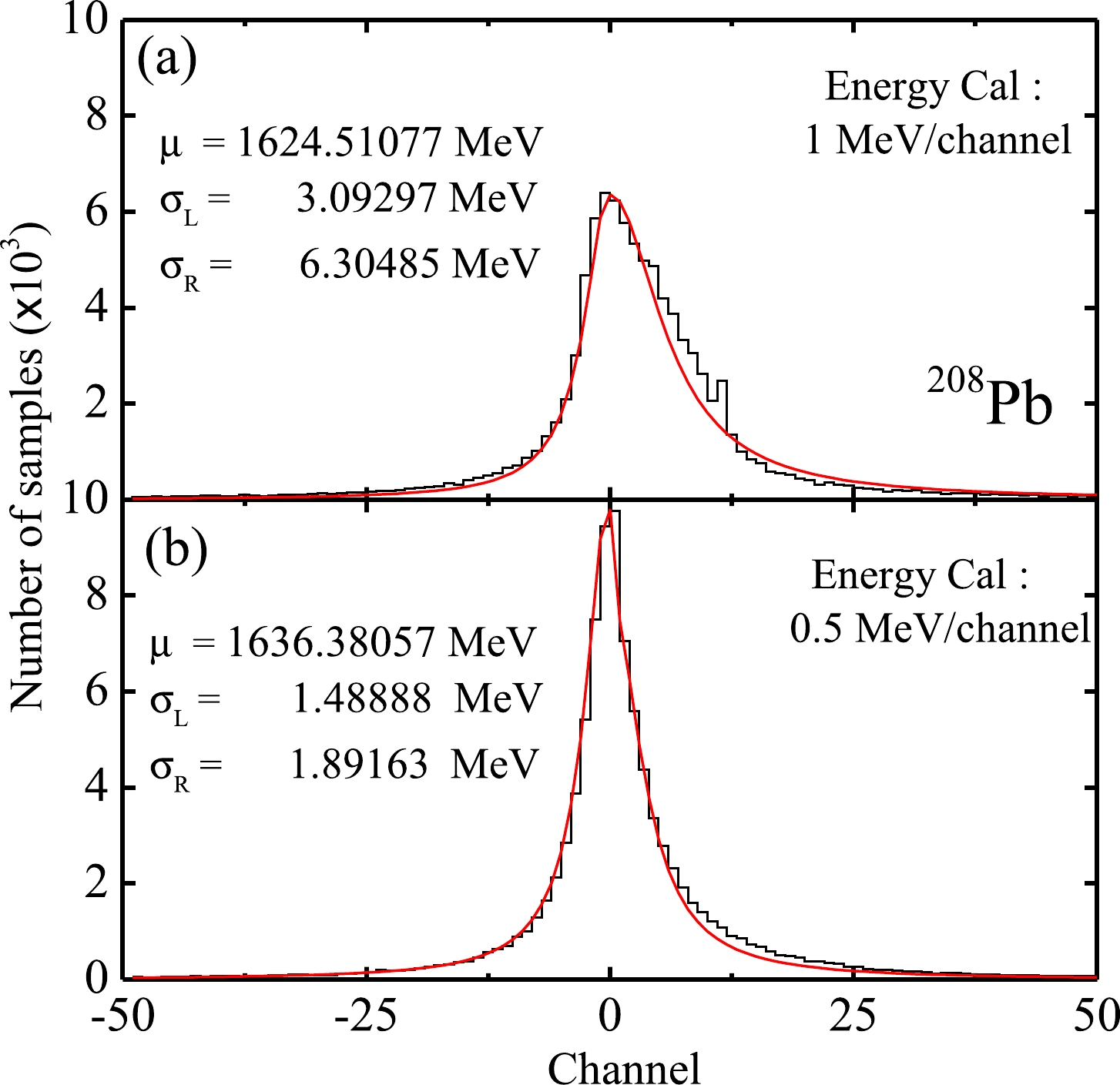

Figure 5.  (color online) (a) Distribution of calculated binding energies for $ ^{208} $Pb from $ 10^5 $ sets of parameters, which are obtained based on the uncorrected experimental data. The solid red line indicates the fitting result with the two-Cauchy-type combining function. (b) Same as (a), but the adopted model parameters are obtained from the theoretically-corrected experimental data. Note that for clarity, similar to Fig. 3, we shift the origins of the horizontal coordinates to the values of the position parameters 1624.51077 and 1636.38057 MeV in (a) and (b), respectively.

To evaluate the deviations $ \Delta B $ ($ \equiv B_{{\rm{Exp}}}-B_{{\rm{Th}}} $) and propagation uncertainties as the nuclei move far from the β-stability line, Fig. 6 presents $ \Delta B $ with error bars using one FWHM (which is just for simplicity and will not affect our conclusions; in principle, the error bars are asymmetric) for the entire $ Z=50 $ Sn isotopic chain. Note that this isotopic chain simultaneously includes more available isotopes both on the neutron-deficient and neutron-rich sides, e.g., cf. Fig. 2. As expected, both the deviations and the corresponding uncertainties generally decrease for nuclei close to the β stability, although this is not a strict rule for global fitting. The conclusions obtained from Fig. 5 appear to be entirely suitable for each individual nucleus. The present method used for extracting the theoretical uncertainties is valid to a large extent. As shown in Fig. 6, most of the data can be covered by the predictions within approximately one FWHM, indicating that the deviations between theory and experiment are not significant (namely, the predictions are reliable) according to statistical theory. For the theoretical prediction with error bars, we temporarily define the ratio $ \Delta B $/FWHM, which is related to the significance level (that is, to what extent the prediction is reliable), to illustrate the predictive power to some extent. In other words, a good prediction should not only have a small deviation $ \Delta B $ between theory and experiment but also a small $ |\Delta B $/FWHM| ratio (in general, $ \lesssim $ 1–2, depending on the given significance level). To evaluate the global property of the 578 available even-even nuclei, we show their $ \Delta B $/FWHM ratios in Fig. 7. Most of these ratios are located between $ +1 $ and $ -1 $. The improvement in the theoretical modeling decreases the $ |\Delta B| $ deviation (e.g., $\sigma_{\rm r.m.s}$ decreases from 3.484 to 1.696 MeV, see Table I); however, the prediction reliability is not destroyed because the corresponding FWHM decreases simultaneously. Therefore, it can be said that the present method provides a relatively reasonable uncertainty (e.g., error bars), improving the predictive power of the model. Improvement in the absolute deviation $ |\Delta B| $ between theory and experiment is not our primary concern at present. This study focuses on the method of estimating a model parameter, its uncertainty, and propagation. There is no doubt that if the model is further improved, a more accurate prediction may be obtained, e.g., with both a smaller deviation $ |\Delta B| $ and a lower ratio $ |\Delta B $/FWHM|. Further tests are desirable.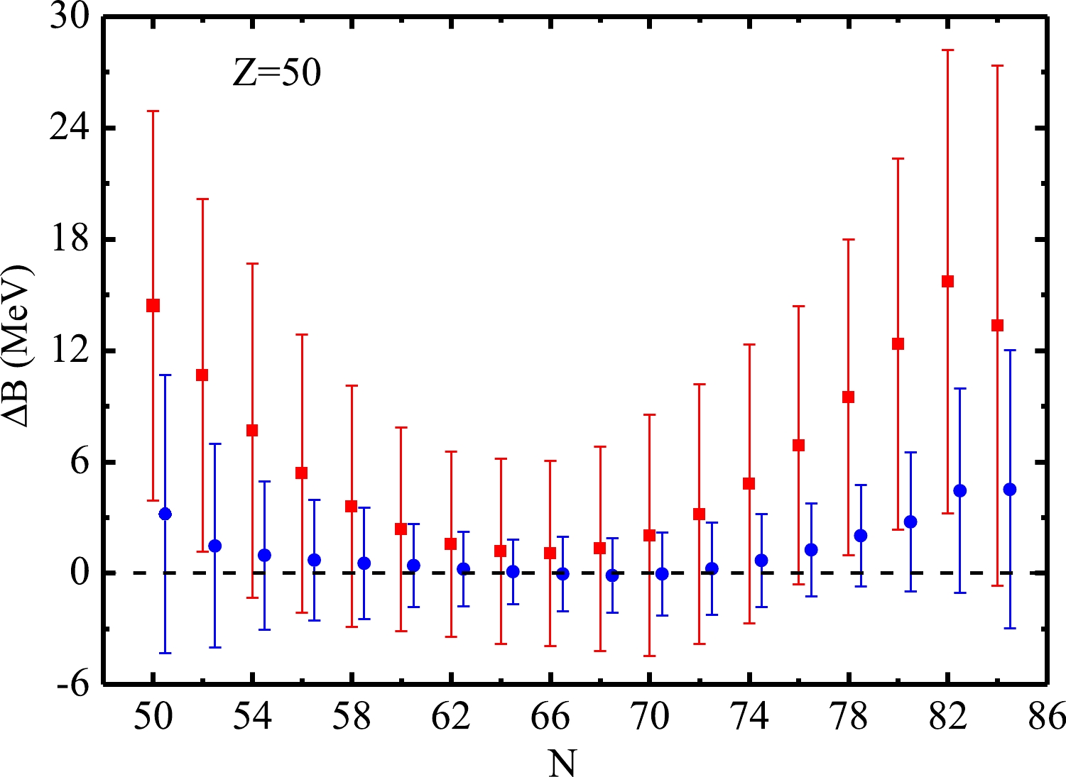

Figure 6.  (color online) Deviations $ \Delta B \pm $FWHM for even-even isotopes $ ^{100-134} $Sn, which are calculated in terms of the model parameters obtained from the uncorrected experimental data (red squares) and theoretically-corrected experimental data (blue circles). To avoid overlapping data, the horizontal coordinates of the blue points are shifted by $ +0.5 $.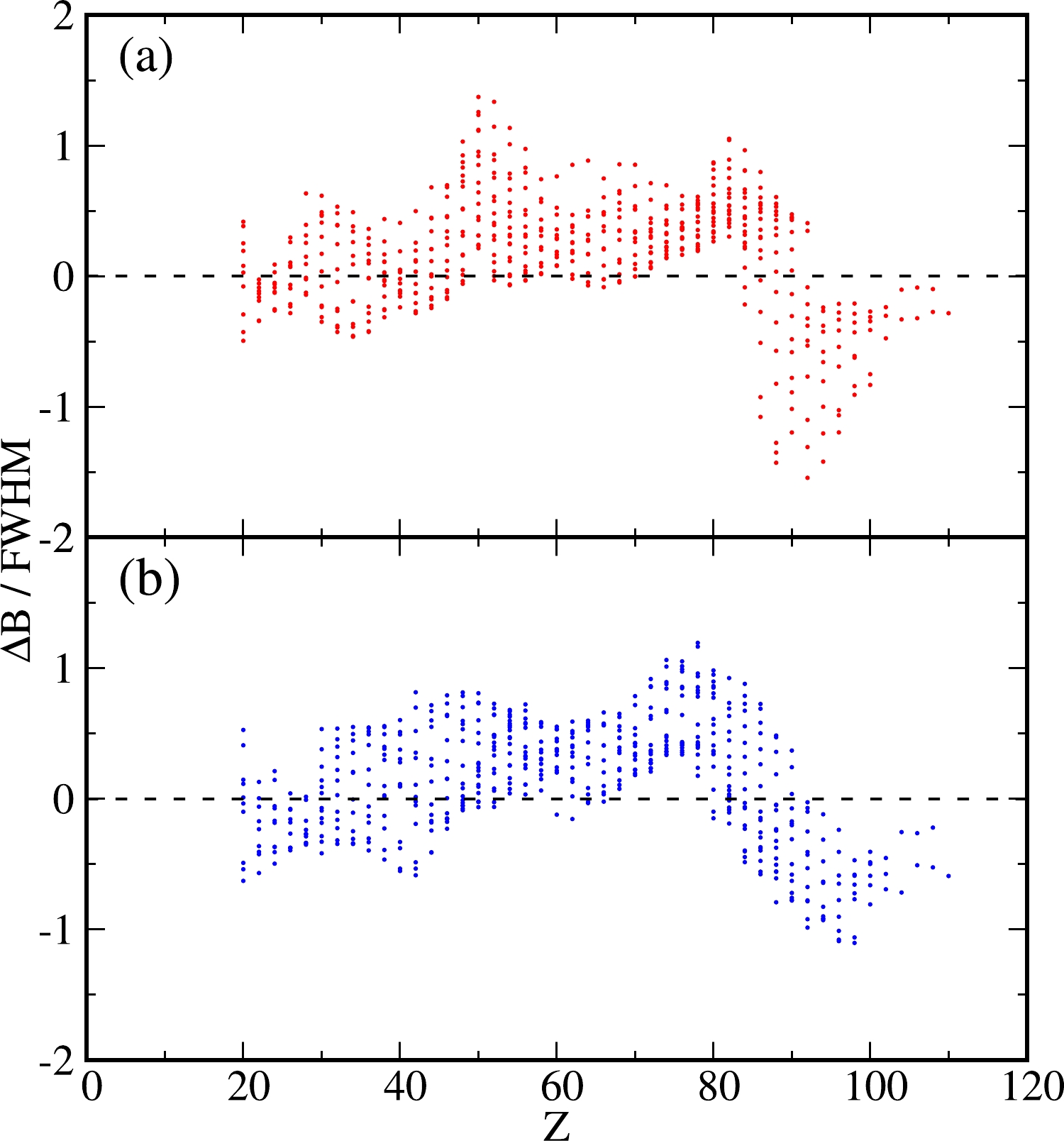

Figure 7.  (color online) (a) Calculated $ \Delta B $/FWHM ratios based on the model parameters obtained from the uncorrected experimental data. (b) Similar to (a), but the used model parameters are based on the theoretically-corrected experimental data.

From a new perspective, we present an estimation method for model parameters and their uncertainties in the macroscopic Bethe-Weizsäcker mass formula and its variant in which the microscopic corrections are considered. Based on $ 10^5 $ Monte Carlo replications and the maximum likelihood estimation, the properties of the Cauchy distribution of model parameters are obtained. We also compare the estimations with the likelihood and least squares estimations, revealing good agreement between the parameter values. Indeed, as expected, we obtain relatively "accurate" values of macroscopic model parameters if the microscopic corrections are subtracted from the adopted experimental data. The predictive power of the model can be improved by considering both the correct parameter correlations and reasonable theoretical modeling. This method can directly provide parameter uncertainties without any pre-assumptions. It will be interesting to extend this method to nuclear physics and other fields if the overdetermined system can be divided into numerous subsystems, which can be exactly solved. Moreover, the physics behind the parameter distribution of the Cauchy line shape is worth investigating in the future.