


 Abstract
 HTML
HTML Reference
 Related
 PDF
PDF


-
Black holes (BHs) and wormholes (WHs) are two fascinating solutions of general relativity (GR). Evidence of BHs has already been shown in literature [1–3] and is established beyond doubt. The discovery of gravity waves and the signatures they carry may soon bring BHs and their study into the domain of observational astrophysics. The presence of WHs has not yet been established, and even their existence is highly debatable. A detailed study has been performed on their existence in [4]. There is a fundamental difference between these entities. BH formation is generic and omnipresent in nature, caused by the gravitational collapse of stars. There is no special requirement regarding the matter content that facilitates the formation of BHs, and the energy conditions are very much preserved in their formation. In contrast, WHs are not sufficiently generic and require a special ecosystem in terms of energy conditions for their formation. WHs require non trivial matter (exotic matter that violates the null energy condition (NEC)) content for their maintenance and formation [5].
After the discovery of BHs and the possibility of probing the interior of BHs via gravity waves, research on WHs increased [6]. WHs and their conception stem from the "Einstein-Rosen bridge" [7], which was initially thought of only as a formal mathematical result. In [8], Wheeler highlighted the theoretical possibility of using a WH to form a bridge between two vastly separated regions. In 1988, Morris and Thorne [9] discovered another class of WH solutions that maintains the WH throat and hence may be traversable. The throat of these WHs is kept open due to a specific type of matter that violates various energy conditions, especially the NEC.
This type of matter is known as exotic matter, which is not part of the standard model of particle physics, and is studied in standard model extensions. It is required in both dynamic [10–13] and static [14–16] WH scenarios. In general, classical matter content satisfies all energy conditions; however, if the effects of quantum theory are included in, for example, the Casimir effect, there are situations in which the energy conditions are violated. Similarly, for quantum gravity, one can encounter scenarios in which classical energy conditions break down, leading to a 'repulsive' big bounce. To quantify the extent of energy violation, Visser et al., in [17], designed the volume integral quantifier (VIQ) to quantify the total averaged null energy condition (ANEC). Moreover, Visser [18, 19] proposed a copy-paste technique to minimize the usage of exotic matter, though this technique is applicable to exotic fluid at the throat of a WH. Kuhfittig gave another solution in [20, 21], where by imposing the condition
$ b^{'}(r)\leq 1 $ (where$ b(r) $ is the shape function) at the WH throat, the region demanding exotic matter can be made arbitrarily small.In recent years, modified theories of gravity have attracted the interest of researchers. These theories are geometrical extensions of Einstein's GR and are used to describe early and late time acceleration of the universe. Significant work has already been conducted on astrophysical objects such as WHs in modified theories, and research is ongoing. Born-Infield theory [22–24], Rastall theory [25], quadratic gravity [26], curvature matter coupling [27–29], Einstein-Cartan gravity [30–32], and braneworld [33–37] are a few examples.
Lobo and Oliveira [38] investigated WH geometries in the context of
$ f(R) $ gravity (where R is the Ricci scalar). They used specific shape functions and various equations of state (EoSs) to find exact WH solutions and studied their behavior with energy condition. In [39], Azizi studied WH geometries in$ f(R,T) $ gravity and revealed the effective stress-energy responsible for the violation of the NEC. Moreover, an interesting study on teleparallel gravity was conducted by Bahamonde et al. in Ref. [40]. Additional articles on WH geometries in different modified theories of gravity, such as in$ f(R,T) $ gravity [41–44],$ f(T) $ gravity [45–47], and$ f(T,T_G) $ gravity [48, 49], are available. A good model outlining the solutions of humanly traversable WHs when generalizing physics beyond the standard model of particle physics using the Randall Sundram model was given by Maldacena [50].Note that the role of the EoS in cosmology is significant because it portrays a physical fluid, which is vital to sustaining geometry. Fluid with a linear EoS and positive energy density is an excellent candidate for describing the expansion of the universe. Furthermore, phantom energy is considered a possible choice to describe the accelerated expansion of the universe and is referred to as
$ \omega=p/\rho<-1 $ . Caldwell first presented this concept in [51]. Because phantom energy violates the NEC, which is necessary for a traversable WH, this energy may play a vital role in forming WHs like spacetime. In [52–55], the authors investigated the physical properties of WHs by considering phantom energy in the context of GR.Recently, Jimenez et al. [56] introduced a new class of modified gravity, known as symmetric teleparallel gravity or
$ f(Q) $ gravity, where Q is a non-metricity scalar. In this theory, both torsion and curvature disappear, and hence gravity only depends on non-metricity. The affine connection plays a significant role in symmetric teleparallel gravity, rather than physical manifold [56]. It is also noted that$ f(Q) $ gravity is attributed to second-order field equations, whereas$ f(R) $ gravity has fourth-order field equations [57]. Hence,$ f(Q) $ gravity offers an alternate geometric portrayal of gravity, which is regardless equivalent to GR. Articles on cosmological [58–60] and astrophysical [61–65] objects are available, in which the authors extensively investigate this symmetric teleparallel gravity.Yixin et al. [66] presented an extension of
$ f(Q) $ gravity, known as$ f(Q,T) $ gravity, which is based on the coupling of non-metricity Q and the trace of the energy-momentum tensor T. In this theory, the gravitational effect is connected through the non-metricity function Q and manifestations from the quantum field owing to the trace of the energy-momentum tensor T. Because it was only recently proposed, significant work has already been done on this gravity based on theoretical [67, 68] and observational [69] aspects. Harko et al. studied novel couplings between non-metricity and matter in [70] and discussed coupling matter in modified Q gravity in [71]. Delhom [72] investigated minimal coupling in the presence of torsion and non-metricity. Moreover,$ f(R) $ gravity, torsion, and non-metricity were studied by Sotiriou in [73].Motivated by the above studies, we intend to study WH solutions in
$ f(Q,T) $ gravity for the spherically symmetric and static configuration. We further extend our analysis by considering (i) a linear EoS relation and (ii) a relation between radial and tangential pressures under the anisotropy case and attempt to find exact WH solutions for both cases using linear and non-linear models.The article is organized as follows. In Sec. II, we show the basic formalism of
$ f(Q,T) $ gravity, and the corresponding field equations for a WH in$ f(Q,T) $ are given in Sec. III. By considering different forms of$ f(Q,T) $ models, we study WH solutions in Sec. IV. A stability analysis of the obtained WH solutions using the Tolman-Oppenheimer-Volkov (TOV) equation is discussed in Sec. V, followed by final remarks in Sec. VI. -
We consider the action for symmetric teleparallel gravity proposed in [66],
$ \begin{equation} \mathcal{S}=\int\frac{1}{16\pi}\,f(Q,T)\sqrt{-g}\,{\rm d}^4x+\int \mathcal{L}_m\,\sqrt{-g}\,{\rm d}^4x\, , \end{equation} $

(1) where
$ f(Q,T) $ is a function of non-metricity Q and the trace of the energy momentum tensor T, g is the determinant of the metric$ g_{\mu\nu} $ , and$ \mathcal{L}_m $ is the matter Lagrangian density.The non-metricity tensor is given by [56]
$ \begin{equation} Q_{\lambda\mu\nu}=\bigtriangledown_{\lambda} g_{\mu\nu}, \end{equation} $

(2) and we can define the non-metricity conjugate or superpotential as
$ \begin{equation} P^\alpha\;_{\mu\nu}=\frac{1}{4}\left[-Q^\alpha\;_{\mu\nu}+2Q_{(\mu}\;^\alpha\;_{\nu)}+Q^\alpha g_{\mu\nu}-\tilde{Q}^\alpha g_{\mu\nu}-\delta^\alpha_{(\mu}Q_{\nu)}\right], \end{equation} $

(3) where
$ \begin{equation} Q_{\alpha}=Q_{\alpha}\;^{\mu}\;_{\mu},\; \tilde{Q}_\alpha=Q^\mu\;_{\alpha\mu}, \end{equation} $

(4) are two traces of the non-metricity tensor.
The non-metricity scalar is represented as [56]
$ Q = -Q_{\alpha\mu\nu}\,P^{\alpha\mu\nu} $

(5) $ \quad = -g^{\mu\nu}\left(L^\beta_{\,\,\,\alpha\mu}\,L^\alpha_{\,\,\,\nu\beta}-L^\beta_{\,\,\,\alpha\beta}\,L^\alpha_{\,\,\,\mu\nu}\right), $

(6) where the disformation
$ L^\beta_{\,\,\,\mu\nu} $ is defined by$ \begin{equation} L^\beta_{\,\,\,\mu\nu}=\frac{1}{2}Q^\beta_{\,\,\,\mu\nu}-Q_{(\mu\,\,\,\,\,\,\nu)}^{\,\,\,\,\,\,\beta}. \end{equation} $

(7) Now, by varying the action with respect to the metric tensor
$ g_{\mu\nu} $ , we can arrive at the gravitational equations of motion, which can be expressed as$ \begin{aligned}[b]& \frac{-2}{\sqrt{-g}}\bigtriangledown_\alpha\left(\sqrt{-g}\,f_Q\,P^\alpha\;_{\mu\nu}\right)-\frac{1}{2}g_{\mu\nu}f +f_T \left(T_{\mu\nu} +\Theta_{\mu\nu}\right)\\ &-f_Q\left(P_{\mu\alpha\beta}\,Q_\nu\;^{\alpha\beta}-2\,Q^ {\alpha\beta}\,\,_{\mu}\,P_{\alpha\beta\nu}\right)=8\pi T_{\mu\nu}, \end{aligned} $

(8) where
$f_Q=\dfrac{{\rm del}f}{{\rm del}Q}$ , and$f_T=\dfrac{{\rm del}f}{{\rm del}T}$ .By definition, the energy-momentum tensor for a fluid depiction of spacetime can be composed of
$ \begin{equation} T_{\mu\nu}=-\frac{2}{\sqrt{-g}}\frac{\delta\left(\sqrt{-g}\,\mathcal{L}_m\right)}{\delta g^{\mu\nu}}, \end{equation} $

(9) and
$ \begin{equation} \Theta_{\mu\nu}=g^{\alpha\beta}\frac{\delta T_{\alpha\beta}}{\delta g^{\mu\nu}}. \end{equation} $

(10) -
Consider a spherically symmetric and static WH metric in Schwarzschild coordinates
$ (t,\,r,\,\theta,\,\Phi) $ , given by [5, 9]$ \begin{equation} {\rm d}s^2=e^{2\phi(r)}{\rm d}t^2-\left(1-\frac{b(r)}{r}\right)^{-1}{\rm d}r^2-r^2\,{\rm d}\theta^2-r^2\,\sin^2\theta\,{\rm d}\Phi^2, \end{equation} $

(11) where
$ \phi(r) $ and$ b(r) $ denote the redshift and shape functions, respectively. They both obey the following conditions [5, 9]:$ (1) $ For$ r>r_0 $ , i.e., out of the throat,$1-\dfrac{b(r)}{r} > 0$ . At the WH throat, i.e.,$ r=r_0 $ ,$ b(r) $ must satisfy the condition$ b(r_0)=r_0 $ .$ (2) $ The shape function$ b(r) $ must fulfill the flaring-out requirement at the throat, i.e.,$ b'(r_0)<1 $ .$ (3) $ For the asymptotic flatness condition, the limit$\dfrac{b(r)}{r}\rightarrow 0$ as$ r\rightarrow \infty $ is required.$ (4) $ The redshift function$ \phi(r) $ should be finite everywhere.In this coordinate system, the nonvanishing components of
$ Q_{\lambda\mu\nu} $ and$ L^{\lambda}_{\,\,\,\mu\nu} $ are$ \begin{aligned}[b] &Q_{rtt}=2\,e^{2\phi}\phi^{'},\,\,\,\,\,Q_{rrr}=-\frac{(rb^{'}-b)}{(r-b)^2},\\& Q_{\theta r \theta}=Q_{\theta\theta r}=-\frac{rb}{r-b},\,\,\,\,Q_{\Phi r \Phi}=Q_{\Phi\Phi\,r}=-\frac{rb\sin^2\theta}{r-b}, \end{aligned} $

(12) and
$ \begin{aligned}[b]& L^{t}_{\,\,t\,r}=L^{t}_{\,\,r\,t}=-\phi^{'},\,\,\,\,L^{r}_{\,\,\theta\theta}=-b,\,\,\,L^{r}_{\,\,t\,t}=-\frac{(r-b)}{r}e^{2\phi}\phi{'},\\&L^{r}_{\,\,r\,r}=-\frac{(rb^{'}-b}{2\,r(r-b)},\,\,L^{r}_{\,\,\Phi\Phi}=-b\sin^2\theta, \end{aligned} $

(13) respectively, where
$ ' $ represents the derivative with respect to the radial coordinate r.In this study, we assume the matter content described by an anisotropic energy-momentum tensor to analyze the WH solutions, which is given by [5, 9]
$ \begin{equation} T_{\mu}^{\nu}=\left(\rho+p_t\right)u_{\mu}\,u^{\nu}-p_t\,\delta_{\mu}^{\nu}+\left(p_r-p_t\right)v_{\mu}\,v^{\nu}, \end{equation} $

(14) where ρ denotes the energy density, and
$ u_{\mu} $ and$ v_{\mu} $ are the four velocity vector and unitary space-like vectors, respectively. Both satisfy the conditions$ u_{\mu}u^{\nu}=-v_{\mu}v^{\nu}=1 $ .$ p_r $ and$ p_t $ denote the radial and tangential pressures, respectively, and are both functions of the radial coordinate r. The trace of the energy-momentum tensor turns out to be$ T=\rho-p_r-2p_t $ .In this article, we consider the matter Lagrangian
$ \mathcal{L}_m=-P $ [74], and hence Eq. (10) can be read as$ \begin{equation} \Theta_{\mu\nu}=-g_{\mu\nu}\,P-2\,T_{\mu\nu}, \end{equation} $

(15) where P is the total pressure and can be expressed as
$P=\dfrac{p_r+2\,p_t}{3}$ .The non-metricity scalar Q for the metric (11) is given by
$ \begin{equation} Q=-\frac{b}{r^2}\left[\frac{rb^{'}-b}{r(r-b)}+2\phi^{'}\right]. \end{equation} $

(16) Now, inserting Eqs. (11), (14), and (16) into the motion equation (Eq. (8)), we obtain the non-zero components of the field equations for
$ f(Q,T) $ gravity.$ \begin{aligned}[b] \\[-7pt] \frac{2 (r-b)}{(2 r-b) f_Q}\Bigg[\rho-\frac{(r-b)}{8 \pi r^3} \Bigg(\frac{b r f_{\rm{QQ}} Q'}{r-b}+b f_Q \Bigg(\frac{ r \phi '+1}{r-b}-\frac{2 r-b}{2 (r-b)^2}\Bigg)+\frac{f r^3}{2 (r-b)}\Bigg)+\frac{f_T (P+\rho )}{8 \pi }\Bigg]=\frac{b'}{8 \pi r^2}, \end{aligned} $ 
(17) $ \frac{2 b}{f r^3}\left[p_r +\frac{(r-b)}{16 \pi r^3} \left(f_Q \left(\frac{b \left(\frac{r b'-b}{r-b}+2 r \phi '+2\right)}{r-b}-4 r \phi '\right)+\frac{2 b r f_{\rm{QQ}} Q'}{r-b}\right)+\frac{fr^3 (r-b)\phi '}{8\pi b r^2}-\frac{f_T \left(P-p_r\right)}{8 \pi }\right] =\frac{1}{8 \pi}\left[2\left(1-\frac{b}{r}\right)\frac{\phi '}{r}-\frac{b}{r^3}\right], $

(18) $ \begin{aligned}[b]& \frac{1}{f_Q \left(\frac{r}{r-b}+r \phi '\right)}\left[p_t +\frac{(r-b)}{32 \pi r^2}\left(f_Q \left(\frac{4 (2 b-r) \phi '}{r-b}-4 r \left(\phi '\right)^2-4 r \phi ''\right)+\frac{2 f r^2}{r-b}-4 r f_{\rm{QQ}} Q' \phi '\right) \right.\\& \left. +\frac{(r-b)}{8\pi r}\left(\phi '' +{\phi '}^2-\frac{(rb'-b)\phi '}{2r(r-b)}+\frac{\phi '}{r}\right)f_Q \left(\frac{r}{r-b}+r \phi '\right)-\frac{f_T \left(P-p_t\right)}{8 \pi }\right]\\ =&\frac{1}{8\pi}\left(1-\frac{b}{r}\right)\left[\phi '' +{\phi '}^2-\frac{(rb'-b)\phi '}{2r(r-b)}-\frac{rb'-b}{2r^2 (r-b)}+\frac{\phi '}{r}\right]. \end{aligned} $

(19) It is known that the Morris-Throne traversable WH field equations for GR can be written as
$ \begin{equation} \frac{b'}{8 \pi r^2}= \tilde{\rho}, \end{equation} $

(20) $ \begin{equation} \frac{1}{8 \pi}\left[2\left(1-\frac{b}{r}\right)\frac{\phi '}{r}-\frac{b}{r^3}\right] = \tilde{p_r}, \end{equation} $

(21) $ \begin{equation} \frac{1}{8\pi}\left(1-\frac{b}{r}\right)\left[\phi '' +{\phi '}^2-\frac{(rb'-b)\phi '}{2r(r-b)}-\frac{rb'-b}{2r^2 (r-b)}+\frac{\phi '}{r}\right] = \tilde{p_t}. \end{equation} $

(22) where
$ \tilde{\rho} $ ,$ \tilde{p_r} $ , and$ \tilde{p_t} $ are the corresponding energy density, radial pressure, and tangential pressure, respectively. Comparing Eqs. (17)–(19) with Eqs. (20)–(22), we get$ \begin{aligned}\\[-9pt] \tilde{\rho}=\frac{2 (r-b)}{(2 r-b) f_Q}\left[\rho-\frac{1}{8 \pi r^2}\left(1-\frac{b}{r}\right) \left(\frac{b r f_{\rm{QQ}} Q'}{r-b}+b f_Q \left(\frac{ r \phi '+1}{r-b}-\frac{2 r-b}{2 (r-b)^2}\right)+\frac{f r^3}{2 (r-b)}\right)+\frac{f_T (P+\rho )}{8 \pi }\right], \end{aligned} $

(23) $ \begin{equation} \tilde{p_r}=\frac{2 b}{f r^3}\left[p_r +\frac{1}{16 \pi r^2}\left(1-\frac{b}{r}\right) \left(f_Q \left(\frac{b \left(\frac{r b'-b}{r-b}+2 r \phi '+2\right)}{r-b}-4 r \phi '\right)+\frac{2 b r f_{\rm{QQ}} Q'}{r-b}\right)+\frac{fr^3 (r-b)\phi '}{8\pi b r^2}-\frac{f_T \left(P-p_r\right)}{8 \pi }\right], \end{equation} $

(24) $ \begin{aligned}[b] \tilde{p_t}=&\frac{1}{f_Q \left(\frac{r}{r-b}+r \phi '\right)}\left[p_t +\frac{1}{32 \pi r}\left(1-\frac{b}{r}\right) \left(f_Q \left(\frac{4 (2 b-r) \phi '}{r-b}-4 r \left(\phi '\right)^2-4 r \phi ''\right)+\frac{2 f r^2}{r-b}-4 r f_{\rm{QQ}} Q' \phi '\right) \right.\\& \left. +\frac{1}{8\pi}\left(1-\frac{b}{r}\right)\left(\phi '' +{\phi '}^2-\frac{(rb'-b)\phi '}{2r(r-b)}+\frac{\phi '}{r}\right)f_Q \left(\frac{r}{r-b}+r \phi '\right)-\frac{f_T \left(P-p_t\right)}{8 \pi }\right]. \end{aligned} $

(25) From the above equations, we find extra terms beyond GR equations. Moreover, considering Eqs. (17)–(19), we find that the corresponding field equations for
$ f(Q,T) $ gravity are$ \begin{equation} 8 \pi \rho =\frac{(r-b)}{2 r^3} \left[f_Q \left(\frac{(2 r-b) \left(r b'-b\right)}{(r-b)^2}+\frac{b \left(2 r \phi '+2\right)}{r-b}\right)+\frac{2 b r f_{\rm{QQ}} Q'}{r-b}+\frac{f r^3}{r-b}-\frac{2r^3 f_T (P+\rho )}{(r-b)}\right], \end{equation} $

(26) $ \begin{equation} 8 \pi p_r=-\frac{(r-b)}{2 r^3} \left[f_Q \left(\frac{b }{r-b}\left(\frac{r b'-b}{r-b}+2 r \phi '+2\right)-4 r \phi '\right)+\frac{2 b r f_{\rm{QQ}} Q'}{r-b}+\frac{f r^3}{r-b}-\frac{2r^3 f_T \left(P-p_r\right)}{(r-b)}\right], \end{equation} $

(27) $ \begin{equation} 8 \pi p_t=-\frac{(r-b)}{4 r^2} \left[f_Q \left(\frac{\left(r b'-b\right) \left(\frac{2 r}{r-b}+2 r \phi '\right)}{r (r-b)}+\frac{4 (2 b-r) \phi '}{r-b}-4 r \left(\phi '\right)^2-4 r \phi ''\right)-4 r f_{\rm{QQ}} Q' \phi '+\frac{2 f r^2}{r-b}-\frac{4r^2 f_T \left(P-p_t\right)}{(r-b)}\right]. \end{equation} $

(28) With these field equations, we can study WH solutions by considering different models in
$ f(Q,T) $ gravity.Let us dedicate a few lines to classical energy conditions developed from the Raychaudhuri equations. These conditions are used to discuss the physically realistic matter configuration and are known as the NEC, weak energy condition (WEC), dominant energy condition (DEC), and strong energy condition (SEC). They are expressed as follows:
$ \bullet $ WEC if$ \rho\geq0 $ ,$ \rho+p_j\geq0 $ ,$ \forall j $ .$ \bullet $ NEC if$ \rho+p_j\geq0 $ ,$ \forall j $ .$ \bullet $ DEC if$ \rho\geq0 $ ,$ \rho \pm p_j\geq0 $ ,$ \forall j $ .$ \bullet $ SEC if$ \rho+p_j\geq0 $ ,$ \rho+\sum_jp_j\geq0 $ ,$ \forall j $ ,where
$ j=r,\,t $ .It is known that, in GR, the NEC is important because its violation may confirm that exotic matter is present in the WH throat. Hence, the NEC is usually studied for WH solutions in GR. Moreover, energy density must be positive for a realistic matter source that maintains the WH solutions.
Solving Eqs. (26) to (28), we can obtain
$ \begin{aligned}[b] \rho =&-\frac{f_Q f_T \left(-r b' \left(2 r (r-b) \phi '+b+2 r\right)+3 b^2+4 r (b-r) \left(\phi ' \left(r (b-r) \phi '+3 b-2 r\right)+r (b-r) \phi ''\right)\right)}{48 \pi r^3 (r-b) \left(f_T+8 \pi \right)}\\& -\frac{24 \pi f_Q \left(r (b-2 r) b'+b \left(2 r (b-r) \phi '+b\right)\right)}{48 \pi r^3 (r-b) \left(f_T+8 \pi \right)}\\& -\frac{r (b-r) \left(f_T \left(2 f_{\rm{QQ}} Q' \left(2 r (b-r) \phi '+b\right)+3 f r^2\right)+24 \pi \left(2 b f_{\rm{QQ}} Q'+f r^2\right)\right)}{48 \pi r^3 (r-b) \left(f_T+8 \pi \right)}, \end{aligned} $ 
(29) $ \begin{aligned}[b] p_r=&\frac{f_Q f_T \left(r b' \left(2 r (r-b) \phi '+b+2 r\right)-3 b^2-4 r (b-r) \left(\phi ' \left(r (b-r) \phi '+3 b-2 r\right)+r (b-r) \phi ''\right)\right)}{48 \pi r^3 (b-r) \left(f_T+8 \pi \right)}\\& +\frac{24 \pi f_Q \left(b r b'-(3 b-2 r) \left(2 r (b-r) \phi '+b\right)\right)}{48 \pi r^3 (b-r) \left(f_T+8 \pi \right)}\\& -\frac{r (b-r) \left(f_T \left(2 f_{\rm{QQ}} Q' \left(2 r (b-r) \phi '+b\right)+3 f r^2\right)+24 \pi \left(2 b f_{\rm{QQ}} Q'+f r^2\right)\right)}{48 \pi r^3 (b-r) \left(f_T+8 \pi \right)}, \end{aligned} $

(30) $ \begin{aligned}[b] p_t=&-\frac{f_Q f_T \left(-r b' \left(2 r (r-b) \phi '+b+2 r\right)+3 b^2+4 r (b-r) \left(\phi ' \left(r (b-r) \phi '+3 b-2 r\right)+r (b-r) \phi ''\right)\right)}{48 \pi r^3 (b-r) \left(f_T+8 \pi \right)}\\& -\frac{24 \pi r f_Q \left(r \left(b' \left((b-r) \phi '-1\right)+2 (b-r)^2 \left(\left(\phi '\right)^2+\phi ''\right)+(2 r-5 b) \phi '\right)+b \left(3 b \phi '+1\right)\right)}{48 \pi r^3 (b-r) \left(f_T+8 \pi \right)}\\& -\frac{r (b-r) \left(f_T \left(2 b f_{\rm{QQ}} Q'+3 f r^2\right)+4 r (b-r) f_{\rm{QQ}} \left(f_T+12 \pi \right) Q' \phi '+24 \pi f r^2\right)}{48 \pi r^3 (b-r) \left(f_T+8 \pi \right)}. \end{aligned} $

(31) These equations, therefore, establish the following constraints on the energy conditions:
$ \bullet $ WEC :$ \begin{aligned}[b] \rho =& -\frac{f_Q f_T \left(-r b' \left(2 r (r-b) \phi '+b+2 r\right)+3 b^2+4 r (b-r) \left(\phi ' \left(r (b-r) \phi '+3 b-2 r\right)+r (b-r) \phi ''\right)\right)}{48 \pi r^3 (r-b) \left(f_T+8 \pi \right)}\\ &-\frac{24 \pi f_Q \left(r (b-2 r) b'+b \left(2 r (b-r) \phi '+b\right)\right)}{48 \pi r^3 (r-b) \left(f_T+8 \pi \right)}\\& -\frac{r (b-r) \left(f_T \left(2 f_{\rm{QQ}} Q' \left(2 r (b-r) \phi '+b\right)+3 f r^2\right)+24 \pi \left(2 b f_{\rm{QQ}} Q'+f r^2\right)\right)}{48 \pi r^3 (r-b) \left(f_T+8 \pi \right)}\geq0,\\ \rho + p_r =& \frac{f_Q \left(r b'+2 r (r-b) \phi '-b\right)}{r^3 \left(f_T+8 \pi \right)}\geq0 ,\\ \rho + p_t =& \frac{f_Q \left(r \left(b' \left(1-r \phi '\right)+2 r (r-b) \left(\left(\phi '\right)^2+\phi ''\right)-\left((b-2 r) \phi '\right)\right)+b\right)+2 r f_{\rm{QQ}} Q' \left(r (r-b) \phi '+b\right)}{2 r^3 \left(f_T+8 \pi \right)}\geq0. \end{aligned} $

(32) $ \bullet $ NEC :$ \begin{aligned}[b] \rho + p_r =& \frac{f_Q \left(r b'+2 r (r-b) \phi '-b\right)}{r^3 \left(f_T+8 \pi \right)}\geq0 ,\\ \rho + p_t =& \frac{f_Q \left(r \left(b' \left(1-r \phi '\right)+2 r (r-b) \left(\left(\phi '\right)^2+\phi ''\right)-\left((b-2 r) \phi '\right)\right)+b\right)+2 r f_{\rm{QQ}} Q' \left(r (r-b) \phi '+b\right)}{2 r^3 \left(f_T+8 \pi \right)}\geq0. \end{aligned} $

(33) $ \bullet $ DEC :$ \begin{aligned}[b] \rho =& -\frac{f_Q f_T \left(-r b' \left(2 r (r-b) \phi '+b+2 r\right)+3 b^2+4 r (b-r) \left(\phi ' \left(r (b-r) \phi '+3 b-2 r\right)+r (b-r) \phi ''\right)\right)}{48 \pi r^3 (r-b) \left(f_T+8 \pi \right)}\\ &-\frac{24 \pi f_Q \left(r (b-2 r) b'+b \left(2 r (b-r) \phi '+b\right)\right)}{48 \pi r^3 (r-b) \left(f_T+8 \pi \right)}\\& -\frac{r (b-r) \left(f_T \left(2 f_{\rm{QQ}} Q' \left(2 r (b-r) \phi '+b\right)+3 f r^2\right)+24 \pi \left(2 b f_{\rm{QQ}} Q'+f r^2\right)\right)}{48 \pi r^3 (r-b) \left(f_T+8 \pi \right)}\geq0,\\ \rho - p_r =& \frac{f_Q f_T \left(r b' \left(2 r (r-b) \phi '+b+2 r\right)-3 b^2-4 r (b-r) \left(\phi ' \left(r (b-r) \phi '+3 b-2 r\right)+r (b-r) \phi ''\right)\right)}{24 \pi r^3 (r-b) \left(f_T+8 \pi \right)}\\& +\frac{24 \pi f_Q \left(r^2 b'-(2 b-r) \left(2 r (b-r) \phi '+b\right)\right)}{24 \pi r^3 (r-b) \left(f_T+8 \pi \right)}\\& -\frac{r (b-r) \left(f_T \left(2 f_{\rm{QQ}} Q' \left(2 r (b-r) \phi '+b\right)+3 f r^2\right)+24 \pi \left(2 b f_{\rm{QQ}} Q'+f r^2\right)\right)}{24 \pi r^3 (r-b) \left(f_T+8 \pi \right)}\geq0 ,\end{aligned} $

$ \begin{aligned}[b] \rho - p_t =& -\frac{f_Q f_T \left(-r b' \left(2 r (r-b) \phi '+b+2 r\right)+3 b^2+4 r (b-r) \left(\phi ' \left(r (b-r) \phi '+3 b-2 r\right)+r (b-r) \phi ''\right)\right)}{24 \pi r^3 (r-b) \left(f_T+8 \pi \right)}\\ &-\frac{12 \pi f_Q \left(r b' \left(r (b-r) \phi '+b-3 r\right)+r (b-r) \left(\phi ' \left(2 r (b-r) \phi '+5 b-2 r\right)+2 r (b-r) \phi ''\right)+b (b+r)\right)}{24 \pi r^3 (r-b) \left(f_T+8 \pi \right)}\\& -\frac{r (b-r) \left(f_T \left(2 f_{\rm{QQ}} Q' \left(2 r (b-r) \phi '+b\right)+3 f r^2\right)+24 \pi \left(f_{\rm{QQ}} Q' \left(r (b-r) \phi '+b\right)+f r^2\right)\right)}{24 \pi r^3 (r-b) \left(f_T+8 \pi \right)}\geq0. \end{aligned} $

(34) $ \bullet $ SEC :$ \begin{aligned}[b] \rho + p_r + 2 p_t =& \frac{f_Q f_T \left(-r b' \left(2 r (r-b) \phi '+b+2 r\right)+3 b^2+4 r (b-r) \left(\phi ' \left(r (b-r) \phi '+3 b-2 r\right)+r (b-r) \phi ''\right)\right)}{24 \pi r^3 (r-b) \left(f_T+8 \pi \right)}\\& +\frac{24 \pi f_Q \left(-r b' \left(r (r-b) \phi '+b\right)+b^2+r (b-r) \left(\phi ' \left(2 r (b-r) \phi '+5 b-4 r\right)+2 r (b-r) \phi ''\right)\right)}{24 \pi r^3 (r-b) \left(f_T+8 \pi \right)}\\& +\frac{r (b-r) \left(f_T \left(2 b f_{\rm{QQ}} Q'+3 f r^2\right)+4 r (b-r) f_{\rm{QQ}} \left(f_T+12 \pi \right) Q' \phi '+24 \pi f r^2\right)}{24 \pi r^3 (r-b) \left(f_T+8 \pi \right)}\geq0. \end{aligned} $

(35) -
In this section, we study WH solutions with different functional forms of
$ f(Q,T) $ gravity. We analyze the behaviors of the solutions with energy condition. Moreover, to achieve de Sitter and anti-de Sitter asymptotic behaviors, we consider the redshift function$\phi(r)=\rm constant$ , which is applied throughout this study. -
In this subsection, we consider an EoS (which represents a link between the components of the energy-momentum tensor) to solve field equations and construct WH solutions. Typically, this concept is used in GR to find exact WH solutions. Owing to the complexity of field equations in modified gravity, researchers sometimes fail to obtain exact analytical solutions; hence, they use numerical methods or do not consider an EoS. In literature, the linear EoS
$ p_r=\omega\rho $ is the most common for examining WH solutions. In this study, we investigate WH solutions with the following form of EoS [52, 75]:$ \begin{equation} p_r=\omega\rho, \end{equation} $

(36) where ω is the EoS parameter. In Ref. [76], the authors dubbed asymptotically flat WH solutions with
$ \omega \leq -1 $ as a phantom region EoS. It is mentioned in [63] that obtaining WH solutions with a linear EoS is difficult in symmetric teleparallel gravity. However, in this study, we atempt to obtain exact WH solutions in$ f(Q,T) $ gravity.Inserting Eqs. (29) and (30) into Eq. (36), we get
$ \begin{aligned}[b]& f_Q \left[f_T \left(r (b+2 r) b'-3 b^2\right)+24 \pi \left(b r b'-b (3 b-2 r)\right)\right]\\&-r (b-r) \left[f_T \left(2 b f_{\rm{QQ}} Q'+3 f r^2\right)+24 \pi \left(2 b f_{\rm{QQ}} Q'+f r^2\right)\right]\\=& \omega \Bigg[f_Q \left(f_T \left(3 b^2-r (b+2 r) b'\right)+24 \pi \left(r (b-2 r) b'+b^2\right)\right)\\&+r (b-r) \left(f_T \left(2 b f_{\rm{QQ}} Q'+3 f r^2\right)+24 \pi \left(2 b f_{\rm{QQ}} Q'+f r^2\right)\right)\Bigg]. \end{aligned} $

(37) Solving the above equation for the general form of
$ f(Q,T) $ is not easy; hence, we consider several specific functional forms of$ f(Q,T) $ to find the shape function$ b(r) $ . In this study, we consider two specific forms of$ f(Q,T) $ , linear ($ f(Q,T)=\alpha\,Q+\beta\,T $ [66]) and non-linear ($ f(Q,T)=Q+\lambda\,Q^2+\eta\,T $ [77]), and attempt to find exact WH solutions. After calculations, we find that it is not possible to find exact WH solutions analytically in the non-linear case. However, in the linear case, it is possible. Hence, we consider$ \begin{equation} f(Q,T)=\alpha\,Q+\beta\,T. \end{equation} $

(38) to study WH solutions with a linear EoS, where α and β are free parameters.
Using the above linear functional form of
$ f(Q,T) $ in the field equations (26)–(28), we obtain$ \begin{equation} \rho =\frac{\alpha (12 \pi -\beta ) b'}{3 (4 \pi -\beta ) (\beta +8 \pi ) r^2}, \end{equation} $

(39) $ \begin{equation} p_r=-\frac{\alpha \left(2 \beta r b'-3 \beta b+12 \pi b\right)}{3 (4 \pi -\beta ) (\beta +8 \pi ) r^3}, \end{equation} $

(40) $ \begin{equation} p_t=-\frac{\alpha \left((\beta +12 \pi ) r b'+3 b (\beta -4 \pi )\right)}{6 (4 \pi -\beta ) (\beta +8 \pi ) r^3}. \end{equation} $

(41) From Eqs. (39) and (40) and using the EoS given in Eq. (36), we obtain the shape function as
$ \begin{equation} b\left(r\right)= c r^\eta, \end{equation} $

(42) where
$ \begin{equation} \eta={-\frac{3 (\beta -4 \pi )}{\beta (\omega -2)-12 \pi \omega }}\,\,, \end{equation} $

(43) and c is the integrating constant. Without loss of generality, one can consider
$ c=1 $ .To satisfy the asymptotic flatness conditions, η should be less than
$ 1 $ , i.e.,$ \eta < 1 $ , and hence the possible ranges of ω and β are listed below.From the above table,
$ \omega<-1 $ is found under the phantom region, and$ -1<\omega<0 $ is found under the quintessence region. Because the universe is accelerating, we neglect the region$ \omega\geq0 $ . By considering the ranges of ω and β from the table, we fix several values and show the behavior of the shape functions, as shown in Fig. 1. The shape functions exhibit a positively increasing behavior under asymptotic background. The flaring out condition is also satisfied at the throat of the WH. In this case, the throat radius$ r_0=1 $ . Thus, we can conclude that the shape function satisfies all the necessary conditions for its traversability. Now, by taking Eqs. (38) and (42) into account, we are able to express the energy conditions as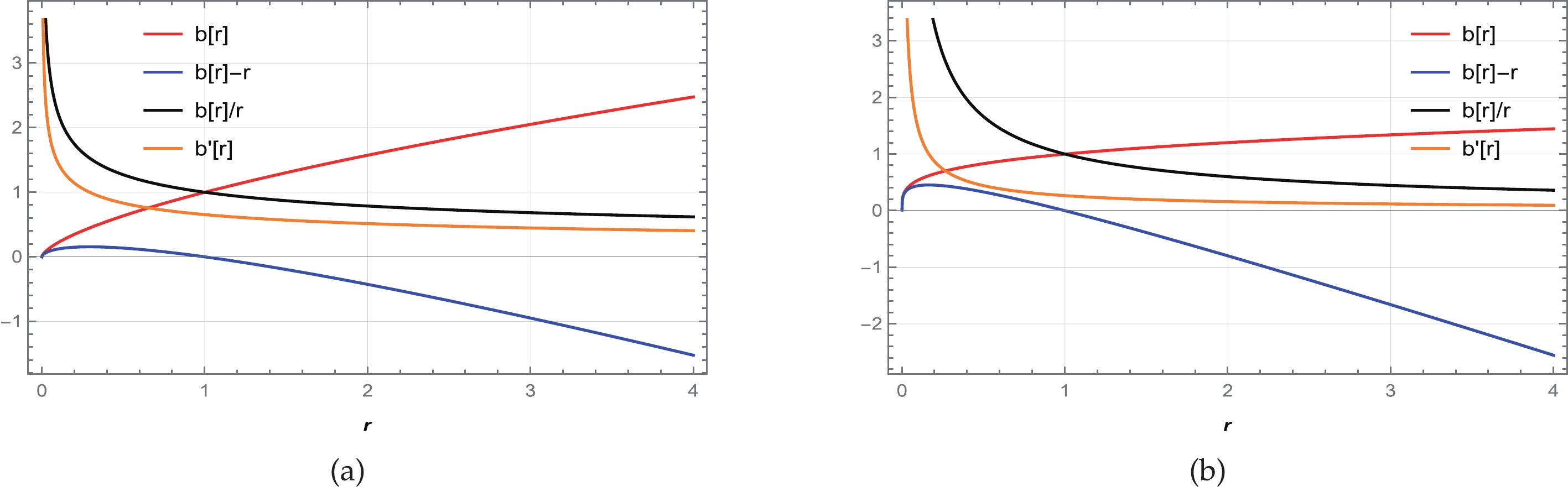
Figure 1. (color online) Behavior of the shape function
$ b(r) $ , flaring out condition$ b'(r)<1 $ , throat condition$ b(r)-r<0 $ , and asymptotic flatness condition$ \frac{b(r)}{r}\rightarrow 0 $ as$ r\rightarrow \infty $ for (a)$ \omega= -1.5 $ with$ \beta=1 $ and (b)$ \omega= -0.5 $ with$ \beta=14 $ . We consider$ \alpha=1 $ and set the unit of radius as kilometers (km).$ \bullet $ NEC :$ \rho+p_r=-\dfrac{\alpha (12 \pi -\beta) (\omega +1) r^{\eta-3}}{\Lambda} $ and$ \rho+p_t=\dfrac{\alpha \left(12 \pi (\omega -1)-\beta (\omega -5)\right) r^{\eta-3}}{2\,\Lambda} $ ,$ \bullet $ DEC :$ \rho-p_r=\dfrac{\alpha (12 \pi -\beta)(\omega -1) r^{\eta-3}}{\Lambda} $ and$ \rho-p_t=-\dfrac{\alpha\,\left(\beta\,(1-\omega) +12 \pi (\omega +3)\right) r^{\eta-3}}{2\,\Lambda} $ ,$ \bullet $ SEC :$\rho+p_r+2p_t=\dfrac{4\,\alpha\,\beta\,r^{\eta-3}}{\Lambda}$ ,where
$ \Lambda=(\beta +8 \pi) \left(12 \pi \omega -\beta (\omega -2)\right) $ .Again, for this linear EoS case, the energy density can be found from the field equation (29),
$ \begin{equation} \rho=\frac{\alpha (\beta -12 \pi ) r^{\eta-3}}{\Lambda}. \end{equation} $

(44) Considering particular values of ω and β based on the obtained ranges, a graph of energy density is plotted in Fig. 2. Figure 2 shows a graph of the energy density ρ for
$ \omega<-1 $ , which indicates that the energy density exhibits a positively decreasing behavior across the entire spacetime. However, for$ -1<\omega<0 $ , it is violating. Therefore, we consider a particular value of$ \omega\in(-\infty, -1) $ and plot graphs for the NEC, DEC, and SEC in Fig. 3. It can be observed from Fig. 3 that the NEC is violated for radial pressure and satisfied for tangential pressure across the entire spacetime. Moreover, the DEC is satisfied for both pressures, whereas the SEC is violated. Violation of the NEC may confirm the presence of exotic matter at the throat of the WH.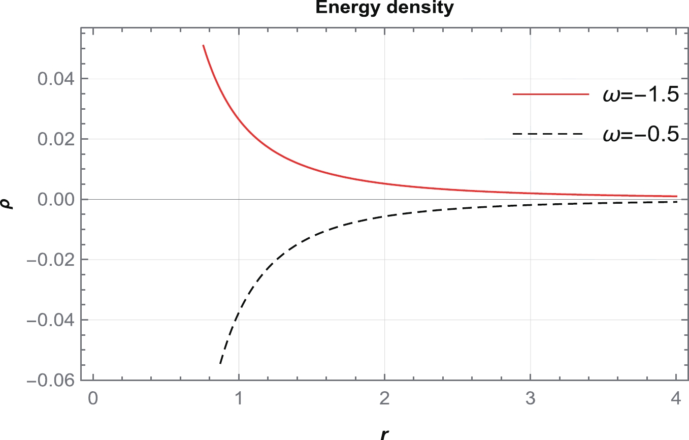
Figure 2. (color online) Behavior of the energy density ρ with respect to r for particular values of
$\omega=-1.5,-0.5$ , corresponding to$\beta=1,14$ , respectively. Here, we consider$\alpha=1$ and set the unit of radius as kilometers (km).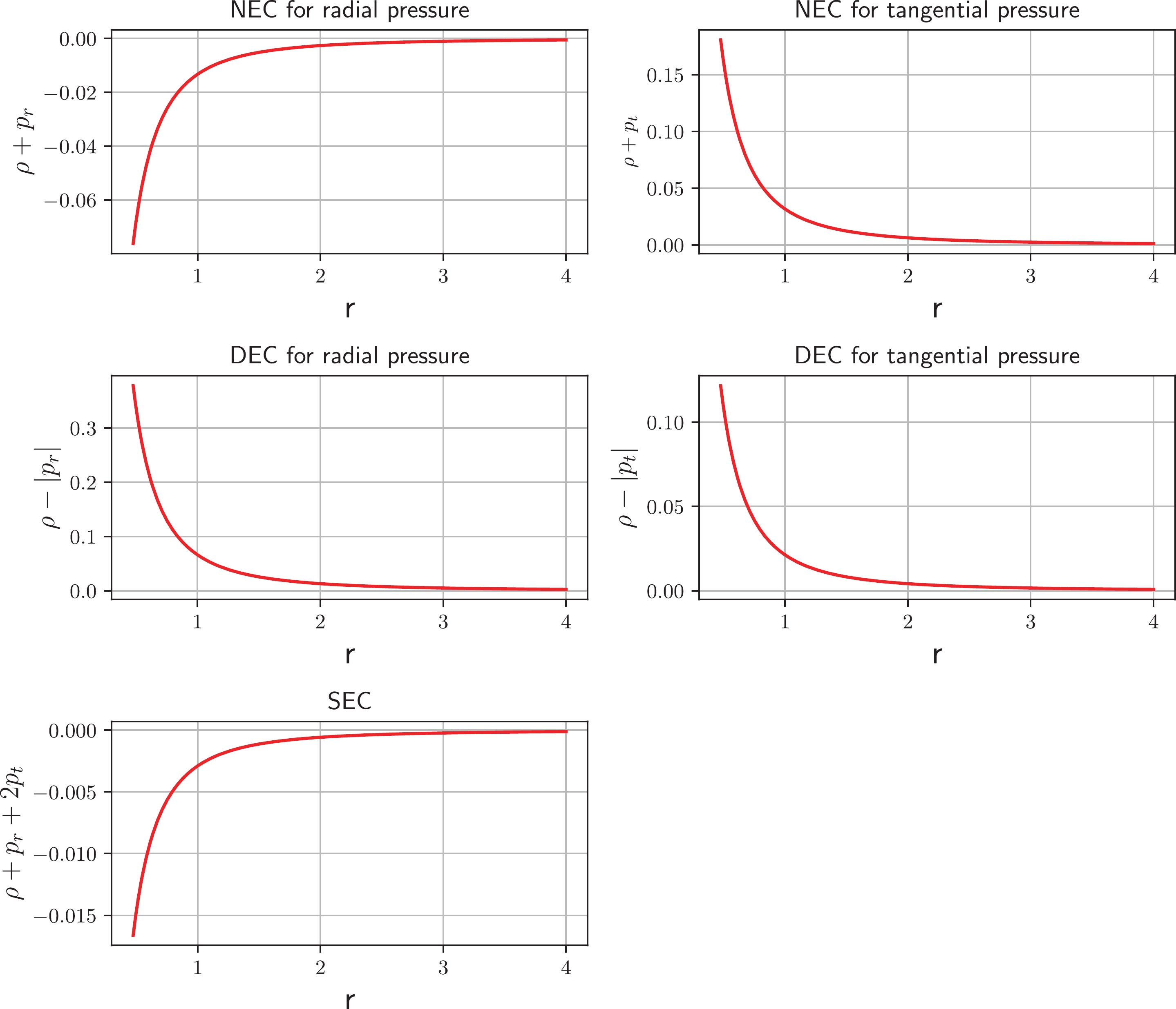
Figure 3. (color online) Behavior of the NEC, DEC, and SEC for
$ \omega=-1.5 $ and$ \beta=1 $ . Here, we consider$ \alpha=1 $ and set the unit of radius as kilometers (km). -
In this section, we consider the anisotropic energy momentum tensor fluid relation
$ p_r\neq p_t $ of the asymptotically flat WH solutions. For this case, we consider the relation between$ p_r $ and$ p_t $ as follows [78, 41]:$ \begin{equation} p_t = n\,p_r, \end{equation} $

(45) where n is any parameter. Because we are studying anisotropic fluid, n cannot be equal to one, i.e.,
$ n\neq1 $ , otherwise it will reduce to a perfect fluid.Inserting Eqs. (30) and (31) into Eq. (45), we get
$ \begin{aligned}[b]& f_Q \Big[(n-1) f_T \left(3 b^2-r (b+2 r) b'\right)\\&+24 \pi \left(r b' (r-b n)+b (3 b n-2 n r-r)\right)\Big]+\\& r (b-r) \Big[2 b f_{\rm{QQ}} Q' \left((n-1) f_T+24 \pi n\right)\\&+3 f (n-1) r^2 \left(f_T+8 \pi \right)\Big]=0. \end{aligned} $

(46) For this case, we use the previous functional forms of
$ f(Q,T) $ and attempt to find the shape function$ b(r) $ . We find that for non-linear$ f(Q,T)=Q+\lambda\,Q^2+\eta\,T $ , the exact WH solutions are formidable owing to the complexity of the field equations. However, for linear$ f(Q,T)=\alpha\,Q+\beta\,T $ , we are able to obtain exact solutions.For the linear case, considering Eqs. (40) and (41) in Eq. (45), we get the shape function
$ b(r) $ as follows:$ \begin{equation} b(r)=c_1 r^{\gamma}, \end{equation} $

(47) where
$ \begin{equation} \gamma=\frac{3 (4 \pi -\beta ) (2 n+1)}{\beta -4 \beta n+12 \pi }, \end{equation} $

(48) and
$ c_1 $ is the integrating constant. Without loss of generality, one can consider$ c_1=1 $ .To satisfy the asymptotic flatness conditions, γ should be less than
$ 1 $ , i.e.,$ \gamma < 1 $ , and hence the possible ranges of n and β are listed below. From the above table, we use particular values of β and n from each domain to plot graphs of shape function in Figs. 4–7. It is clear from the figures that the shape functions satisfy all the necessary conditions for a traversable WH. In this case, we obtain the WH throat radius$ r_0=1 $ .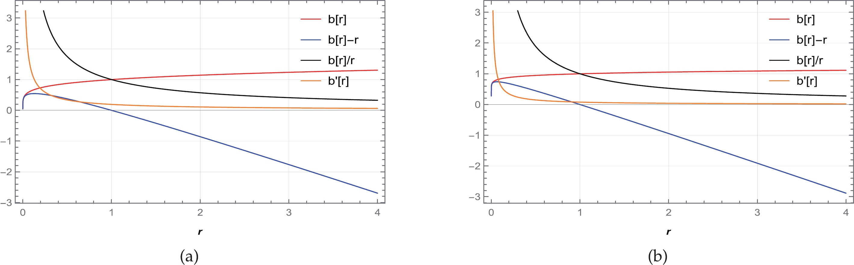
Figure 4. (color online) Behavior of the shape function
$ b(r) $ , flaring out condition$ b'(r)<1 $ , throat condition$ b(r)-r<0 $ , and asymptotic flatness condition$ \frac{b(r)}{r}\rightarrow 0 $ as$ r\rightarrow \infty $ for (a)$ n=-2.5 $ with$ \beta=16 $ and (b)$ n= -2 $ with$ \beta=14 $ . We consider$ \alpha=1 $ and set the unit of radius as kilometers (km).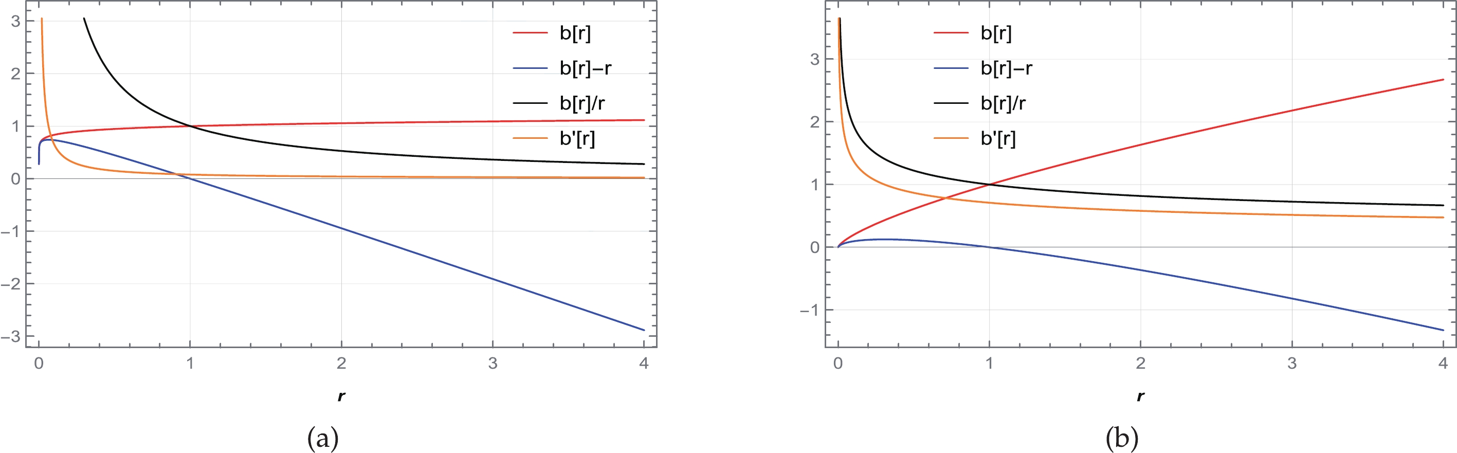
Figure 5. (color online) Behavior of the shape function
$ b(r) $ , flaring out condition$ b'(r)<1 $ , throat condition$ b(r)-r<0 $ , and asymptotic flatness condition$ \frac{b(r)}{r}\rightarrow 0 $ as$ r\rightarrow \infty $ for (a)$ n= -1.5 $ with$ \beta=14 $ and (b)$ n= -0.1 $ with$ \beta=1 $ . We consider$ \alpha=1 $ and set the unit of radius as kilometers (km).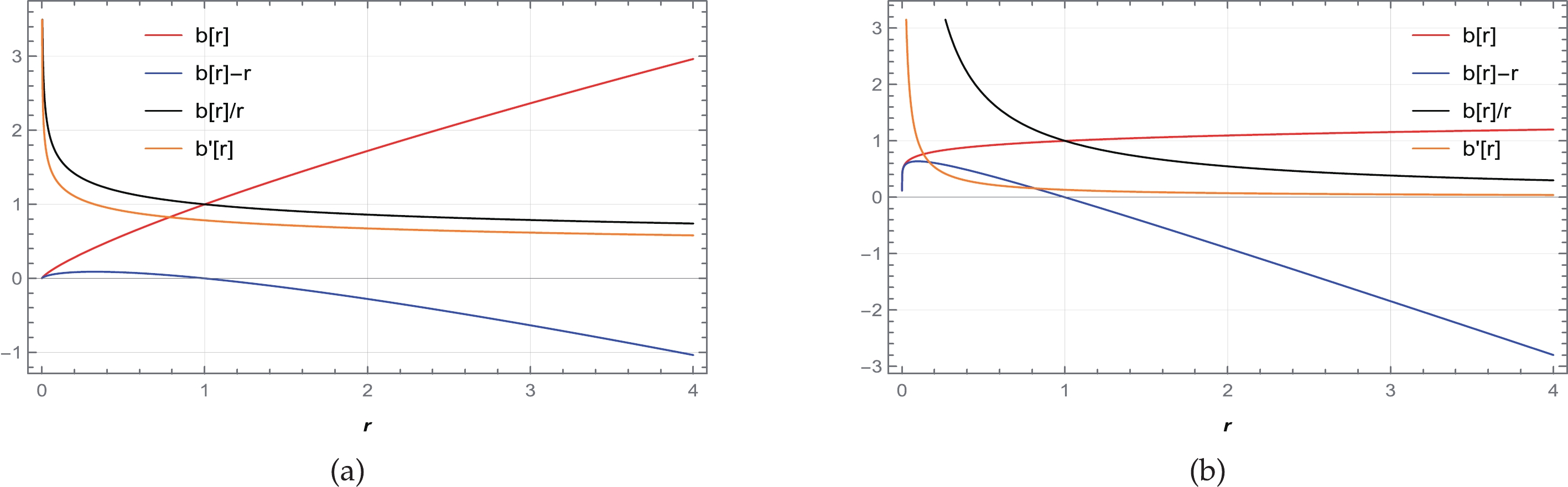
Figure 6. (color online) Behavior of the shape function
$ b(r) $ , flaring out condition$ b'(r)<1 $ , throat condition$ b(r)-r<0 $ , and asymptotic flatness condition$ \frac{b(r)}{r}\rightarrow 0 $ as$ r\rightarrow \infty $ for (a)$ n= 0.25 $ with$ \beta=6 $ and (b)$ n= 0.5 $ with$ \beta=12 $ . We consider$ \alpha=1 $ and set the unit of radius as kilometers (km).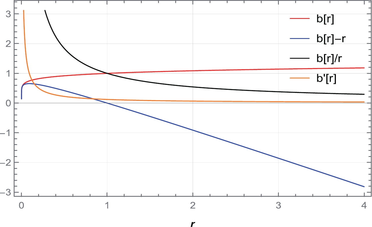
Figure 7. (color online) Behavior of the shape function
$ b(r) $ , flaring out condition$ b'(r)<1 $ , throat condition$ b(r)-r<0 $ , and asymptotic flatness condition$ \frac{b(r)}{r}\rightarrow 0 $ as$ r\rightarrow \infty $ for$ n= 2 $ with$ \beta=13 $ . We consider$ \alpha=1 $ and set the unit of radius as kilometers (km).Again, by considering Eqs. (38) and (47), we obtain the energy conditions defined below.
$ \bullet $ NEC :$ \rho+p_r=\dfrac{r^{k} (24 \pi \alpha n-2 \alpha \beta (n+2))}{\Lambda_{1}} $ and$ \rho+p_t=\dfrac{\alpha (12 \pi (n+1)-\beta (5 n+1)) r^{k}}{\Lambda_{1}} $ ,$ \bullet $ DEC :$ \rho-p_r=\dfrac{2 \alpha (\beta -\beta n+12 \pi (n+1)) r^{k}}{\Lambda_{1}} $ and$ \rho-p_t=\dfrac{\alpha (\beta (n-1)+12 \pi (3 n+1)) r^{k}}{\Lambda_{1}} $ ,$ \bullet $ SEC :$ \rho+p_r+2p_t=-\dfrac{4 \alpha \beta (2 n+1) r^{k}}{\Lambda_{1}} $ ,where
$ \Lambda_{1}=(\beta +8 \pi) (\beta -4 \beta n+12 \pi) $ , and$ k=-\dfrac{6 (\beta +4 \pi) (n-1)}{\beta (4 n-1)-12 \pi } $ .Again, for this case, we find the energy density from the field equation (29),
$ \begin{equation} \rho=\frac{\alpha (12 \pi -\beta ) (2 n+1) r^k}{\Lambda_1}. \end{equation} $

(49) Now, we consider particular values from each domain in Table 3 and plot a graph of energy density, as shown in Fig. 8. We find that energy density is positive for
$ \frac{-1}{2}<n<\frac{1}{4} $ ,$ n=\frac{1}{4} $ , and$ \frac{1}{4}<n<1 $ ; however, for other regions of n, it is violating. Therefore, we consider several particular values of n from$ \frac{-1}{2}<n<\frac{1}{4} $ ,$ n=\frac{1}{4} $ , and$ \frac{1}{4}<n<1 $ and plot graphs for the NEC, DEC, and SEC in Figs. 9–11. It can be observed from Fig. 9 that the NEC is violated for radial pressure and satisfied for tangential pressure across the entire spacetime. Moreover, from Figs. 10 and 11, we conclude that the DEC is satisfied for both pressures, whereas the SEC is violated.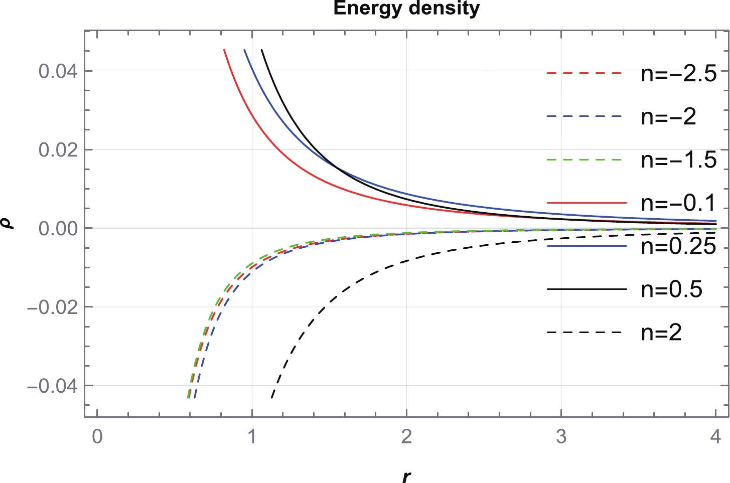
Figure 8. (color online) Behavior of ρ with respect to r for particular values of
$ n=$ –2.5, –2, –1.5, –0.1, 0.25, 0.5, and$ 2 $ , corresponding to$ \beta=$ 16, 14, 14, 1, 6, 12, and$ 13 $ , respectively. We consider$ \alpha=1 $ and set the unit of radius as kilometers (km).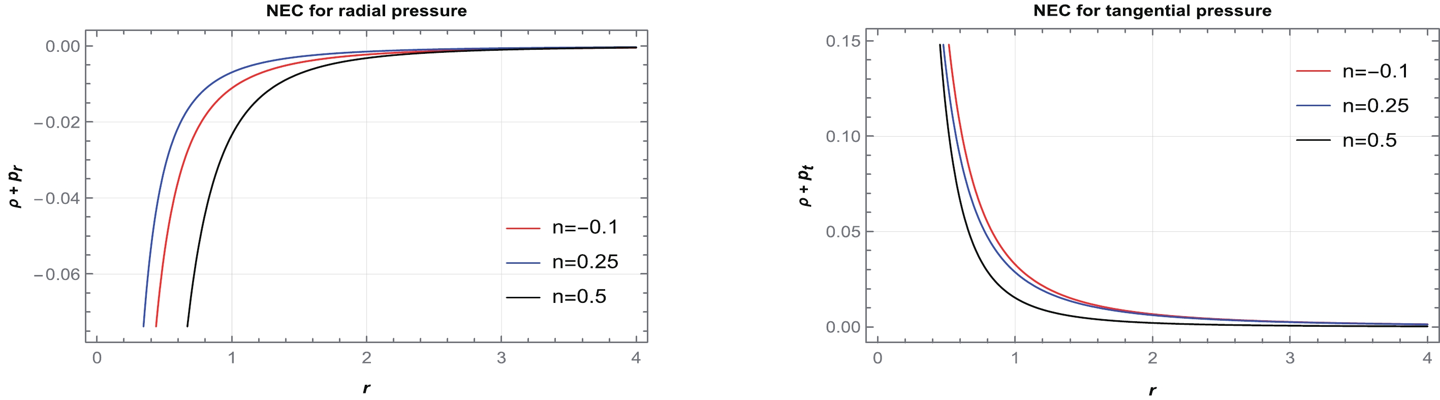
Figure 9. (color online) Behavior of the NEC for
$ n=-0.1,\,0.25, $ and$ 0.5 $ , corresponding to$ \beta=1,\,6, $ and$ 12 $ , respectively. We consider$ \alpha=1 $ and set the unit of radius as kilometers (km).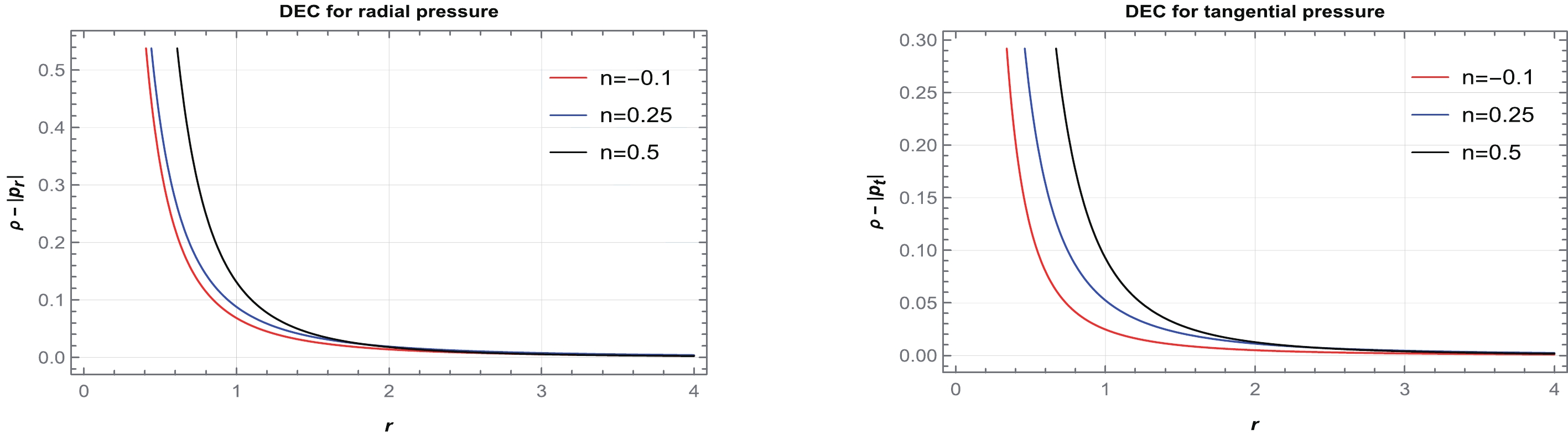
Figure 10. (color online) Behavior of the DEC for
$ n=-0.1,\,0.25, $ and$ 0.5 $ , corresponding to$ \beta=1,\,6, $ and$ 12 $ , respectively. We consider$ \alpha=1 $ and set the unit of radius as kilometers (km).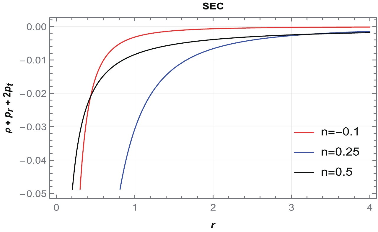
Figure 11. (color online) Behavior of the SEC for
$ n= $ –0.1, 0.25, and$ 0.5 $ , corresponding to$ \beta=1,\,6, $ and$ 12 $ , respectively. We consider$ \alpha=1 $ and set the unit of radius as kilometers (km). -
In this section, we consider the generalized TOV equation [79–81] to find the stability of our obtained WH solutions. The generalized TOV equation can be written as
$ \begin{eqnarray} \frac{\varpi'}{2}(\rho+p_r)+\frac{{\rm d}p_r}{{\rm d}r}+\frac{2}{r}(p_r-p_t)=0, \end{eqnarray} $

(50) where
$ \varpi=2\phi(r) $ .Owing to anisotropic matter distribution, the hydrostatic, gravitational, and anisotropic forces are defined as follows:
$ \begin{eqnarray} F_h=-\frac{{\rm d}p_r}{{\rm d}r}, \; \; \; \; \; F_g=-\frac{\varpi^{'}}{2}(\rho+p_r), \; \; \; \; F_a=\frac{2}{r}(p_t-p_r). \end{eqnarray} $

(51) To place the WH solutions into equilibrium,
$ F_h+F_g+F_a=0 $ must hold. Because, in this study, we assume that the redshift function$\phi(r)=\rm constant$ , it will cause the gravitational contribution$ F_g $ to vanish in the equilibrium equation. Hence, the equilibrium equation becomes$ \begin{equation} F_h+F_a=0. \end{equation} $

(52) Using Eqs. (30), (31), (36), and (38), we obtain the following equations for the hydrostatic and anisotropic forces in the linear model using
$ p_r=\omega \rho $ :$ F_h=-\frac{(\beta -12 \pi ) \omega \left(\dfrac{3 (\beta -4 \pi )}{12 \pi \omega -\beta (\omega -2)}-3\right) r^{\frac{3 (\beta -4 \pi )}{12 \pi \omega -\beta (\omega -2)}-4}}{(\beta +8 \pi ) (12 \pi \omega -\beta (\omega -2))}, $

(53) $ F_a=\frac{3 \alpha (\beta (-\omega )+\beta +4 \pi (3 \omega +1)) r^{\frac{3 (\beta -4 \pi )}{12 \pi \omega -\beta (\omega -2)}-4}}{(\beta +8 \pi ) (12 \pi \omega -\beta (\omega -2))}. $

(54) Furthermore, for the relation
$ p_t=n p_r $ , considering Eqs. (30), (31), (45), and (38), the equations for the hydrostatic and anisotropic forces read as$ \begin{equation} F_h=-\frac{18 \alpha (\beta +4 \pi )^2 (n-1) r^{-\frac{6 (\beta +4 \pi ) (n-1)}{\beta (4 n-1)-12 \pi }-1}}{(\beta +8 \pi ) (\beta -4 \beta n+12 \pi ) (\beta (4 n-1)-12 \pi )}, \end{equation} $

(55) $ \begin{equation} F_a=-\frac{6 \alpha (\beta +4 \pi ) (n-1) r^{-\frac{6 (\beta +4 \pi ) (n-1)}{\beta (4 n-1)-12 \pi }-1}}{(\beta +8 \pi ) (\beta -4 \beta n+12 \pi )}. \end{equation} $

(56) The graphs of hydrostatic and anisotropic forces for both cases are depicted in Figs. 12 and 13. It can be observed that these forces exhibit the same behavior but are opposite to each other. These balanced developments indicate that our obtained WH solutions are stable.
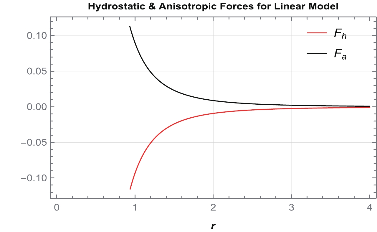
Figure 12. (color online) Behavior of both the hydrostatic and anisotropic forces for
$ p_r=\omega \rho $ with$ \omega=-1.5 $ . We consider$ \alpha=1 $ and set the unit of radius as kilometers (km).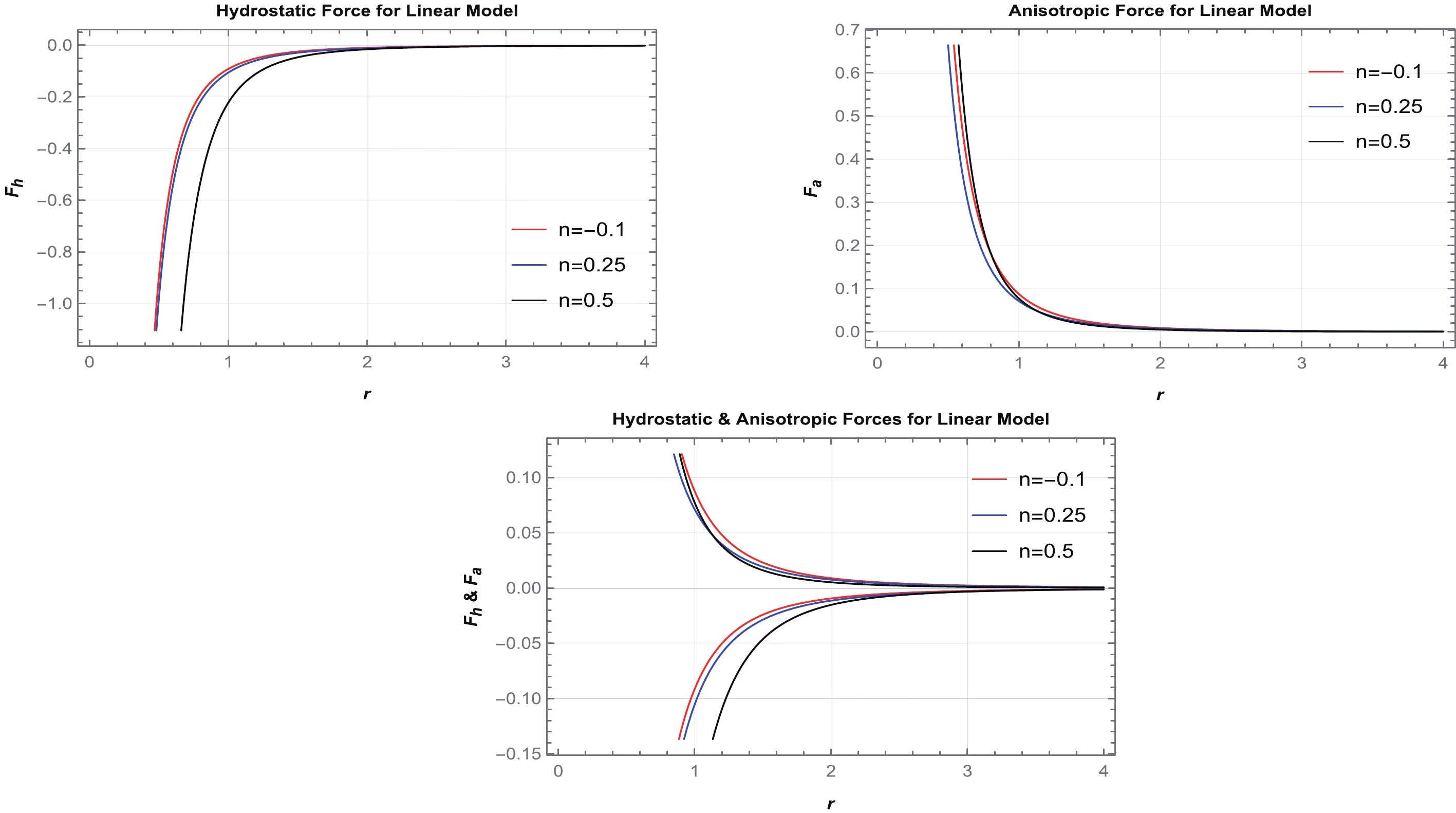
Figure 13. (color online) Behavior of both the hydrostatic and anisotropic forces for
$ p_t=n p_r $ . We consider$ \alpha=1 $ and set the unit of radius as kilometers (km). -
WHs can act as tunnels that connect two spatially different regions separated by a spacelike interval of the same spacetime manifold. They are currently a theoretical possibility that has not yet been observed. Based on advances in gravity wave astronomy, one may be able to conjecture a scenario in which the signatures of an astrophysical WH may be detected. In GR, WH solutions of interest (stable and traversable) suffer from a known pathology where energy conditions are violated. The requirement for exotic matter when one explores standard model extensions in the context of classical GR is a significant hurdle. However, one can now turn to modified versions of gravity to solve issues regarding WHs. The study of WHs in modified theories of gravity makes it possible to derive stable solutions without compromising energy conditions.
The modified theory of gravity
$ f(Q,T) $ has successfully explained late-time acceleration [69] and matter-antimatter asymmetry [68]. It is worth asking whether modified theories of gravity are useful in the context of astrophysical objects such as WHs, and if so, which modified versions support stable, traversable WHs. This is the motivation behind studying WH solutions in the recently proposed$ f(Q,T) $ gravity. Because$ f(Q,T) $ gravity is a novel approach, it may provide new insights into astrophysical objects such as BHs and WHs. In our study, we set up the corresponding field equations in$ f(Q,T) $ gravity. We then conduct our analysis in two phases: (i) WH solutions with a linear EoS, and (ii) anisotropic WH solutions. Furthermore, we study these solutions under two functional forms of the$ f(Q,T) $ model; we consider linear$ f(Q,T)=\alpha\,Q+\beta\,T $ and non-linear$f(Q,T)=Q+ \lambda\,Q^2+ \eta\,T$ . Our aim is to find exact WH solutions for both models. Because our obtained field equations are more complex than solutions in classical GR, finding exact solutions with a linear EoS and an anisotropic relation is a challenging task for both models. We find exact solutions for both cases under the assumption of linear$ f(Q,T) $ . In the case of the non-linear model, finding exact solutions is not analytically feasible for both EoSs. Solutions with the linear EoS for the linear form of$ f(Q,T) $ are obtained explicitly. We find that the shape function is in power-law form. Moreover, to satisfy the asymptotic flatness condition, several domains of ω and β are found, as shown in Table 1. We choose several particular values of ω and β from Table 1 and show the behaviors of the shape functions. We observe that all the necessary conditions of the shape functions are satisfied, which is necessary for a traversable WH. Furthermore, we verify the behavior of energy density in both the phantom and quintessence regions and find that it exhibits a positively decreasing behavior in the phantom region, whereas it is violating in the quintessence region. Keeping this in mind, we choose several particular values of ω and plot graphs of energy conditions. We observe that the NEC is violated for radial pressure and satisfied for tangential pressure. The DEC is satisfied, whereas the SEC is violated, throughout spacetime. In Table 2, we summarize the behavior of the energy conditions.Model Parameters ω β $ (-\infty, -1) $ 

$ \Bigg(-\infty, \dfrac{12 \pi \omega }{\omega -2}\Bigg)\cup (12 \pi, \infty) $ 

$ (-1, 2) $ 

$ \Bigg(\dfrac{12 \pi \omega }{\omega -2}, 12 \pi\Bigg) $ 

$ 2 $ 

$ (-\infty, 12 \pi) $ 

$ (2, \infty) $ 

$ (-\infty, 12 \pi)\cup \Bigg(\dfrac{12 \pi \omega }{\omega -2}, \infty\Bigg) $ 

Table 1. Possible domains of ω and β.
Terms Interpretations ω $ (-\infty, -1) $ 

$ (-1, 2) $ 

β $ \Bigg(-\infty, \dfrac{12 \pi \omega }{\omega -2}\Bigg)\cup (12 \pi, \infty) $ 

$ \Bigg(\dfrac{12 \pi \omega }{\omega -2}, 12 \pi\Bigg) $ 

ρ $ satisfied $ 

$ violated $ 

$ \rho + p_r $ 

$ violated $ 

$ violated $ 

$ \rho + p_t $ 

$ satisfied $ 

$ satisfied $ 

$ \rho - p_r $ 

$ satisfied $ 

$ violated $ 

$ \rho - p_t $ 

$ satisfied $ 

$ violated $ 

$ \rho + p_r + 2p_t $ 

$ violated $ 

$ satisfied $ 

Table 2. Summary of the energy conditions for
$ p_r=\omega\,\rho $ .Furthermore, we study WH solutions for the anisotropic case with both models of
$ f(Q,T) $ . Our analysis shows that for the non-linear model, it is difficult to find exact solutions. However, for the linear model, WH solutions for an anisotropic case are obtained, and we obtain the shape function in power-law form. In Table 3, we show all the possible domains of n and β that satisfy the asymptotic flatness conditions. Figs. 4–7 show that all the necessary conditions of shape functions are satisfied within each of the domains from the table. Moreover, a plot of energy density is depicted in Fig. 8, and we find that for particular values of n, the energy density is positive. Considering these values, we plot graphs of the NEC, DEC, and SEC. It is observed that the NEC and SEC are violated, whereas the DEC is obeyed throughout spacetime in this$ f(Q,T) $ gravity. A summary of the energy conditions for this case is given in Table 4.Model Parameters n β $ (-\infty, -2) $ 

$ \Bigg(\dfrac{12 \pi}{4n-1}, \dfrac{12 \pi n}{n+2}\Bigg) $ 

$ -2 $ 

$ \Bigg(\dfrac{-4 \pi}{3}, \infty\Bigg) $ 

$ \Bigg(-2, \dfrac{-1}{2}\Bigg] $ 

$ \Bigg(-\infty, \dfrac{12 \pi n}{n+2})\Bigg)\cup \Bigg(\dfrac{12 \pi}{4n-1}, \infty\Bigg) $ 

$\Bigg(\dfrac{-1}{2}, \dfrac{1}{4}\Bigg)$ 

$ \Bigg(-\infty, \dfrac{12 \pi}{4n-1}\Bigg) \cup \Bigg(\dfrac{12 \pi n}{n+2}, \infty\Bigg) $ 

$ \dfrac{1}{4} $ 

$ \Bigg(\dfrac{4 \pi}{3}, \infty\Bigg) $ 

$ \Bigg(\dfrac{1}{4}, 1\Bigg) $ 

$ \Bigg(\dfrac{12 \pi n}{n+2}, \dfrac{12 \pi}{4n-1}\Bigg) $ 

$ (1, \infty) $ 

$ \Bigg(\dfrac{12 \pi}{4n-1}, \dfrac{12 \pi n}{n+2}\Bigg) $ 

Table 3. Possible domains of β and n.
Terms Interpretations n $ (-\infty, -2) $ 

$ -2 $ 

$ \Bigg(-2, \dfrac{-1}{2}\Bigg] $ 

$ \Bigg(\dfrac{-1}{2}, \dfrac{1}{4}\Bigg) $ 

$ \dfrac{1}{4} $ 

$ \Bigg(\dfrac{1}{4}, 1\Bigg) $ 

$ (1, \infty) $ 

β $ \Bigg(\dfrac{12 \pi}{4n-1}, \dfrac{12 \pi n}{n+2}\Bigg) $ 

$ \Bigg(\dfrac{-4 \pi}{3}, \infty\Bigg) $ 

$ \Bigg(-\infty, \dfrac{12 \pi n}{n+2}\Bigg)\cup \Bigg(\dfrac{12 \pi}{4n-1}, \infty\Bigg) $ 

$ \Bigg(-\infty, \dfrac{12 \pi}{4n-1}\Bigg) \cup \Bigg(\dfrac{12 \pi n}{n+2}, \infty\Bigg) $ 

$ \Bigg(\dfrac{4 \pi}{3}, \infty\Bigg) $ 

$ \Bigg(\dfrac{12 \pi n}{n+2}, \dfrac{12 \pi}{4n-1}\Bigg) $ 

$ \Bigg(\dfrac{12 \pi}{4n-1}, \dfrac{12 \pi n}{n+2}\Bigg) $ 

ρ $ violated $ 

$ violated $ 

$ violated $ 

$ satisfied $ 

$ satisfied $ 

$ satisfied $ 

$ violated $ 

$ \rho + p_r $ 

$ violated $ 

$ violated $ 

$ violated $ 

$ violated $ 

$ violated $ 

$ violated $ 

$ violated $ 

$ \rho + p_t $ 

$ satisfied $ 

$ satisfied $ 

$ satisfied $ 

$ satisfied $ 

$ satisfied $ 

$ satisfied $ 

$ satisfied $ 

$ \rho - p_r $ 

$ violated $ 

$ satisfied $ 

$ satisfied $ 

$ satisfied $ 

$ satisfied $ 

$ satisfied $ 

$ violated $ 

$ \rho - p_t $ 

$ violated $ 

$ violated $ 

$ violated $ 

$ satisfied $ 

$ satisfied $ 

$ satisfied $ 

$ violated $ 

$ \rho + p_r + 2p_t $ 

$ satisfied $ 

$ satisfied $ 

$ satisfied $ 

$ violated $ 

$ violated $ 

$ violated $ 

$ satisfied $ 

Table 4. Summary of the energy conditions for
$ p_t=n\,p_r $ .For completeness, we check the stability of our obtained WH solutions for both cases. From Figs. 12–13, we can conclude that the obtained WH solutions are stable. Throughout our study, we consider the redshift function
$\phi(r)=\rm constant$ to avoid the presence of an event horizon. It would be interesting to study WH solutions with a non-constant redshift function and different matter sources in$ f(Q,T) $ gravity. -
We are very grateful to the honorable referee and editor for illuminating suggestions that have significantly improved our work in terms of research quality and presentation.
Static spherically symmetric wormholes in $ {\boldsymbol f(\boldsymbol Q,T)} $ gravity
- Received Date: 2022-06-02
- Available Online: 2022-11-15
Abstract: In this study, we obtain wormhole solutions in the recently proposed extension of symmetric teleparallel gravity, known as


 DownLoad: