


 Abstract
 HTML
HTML Reference
 Related
 PDF
PDF


-
$ CP $ violation reflects the asymmetry between matter and antimatter. Since the discovery of$ CP $ violation in the decay process of K mesons, theories and experiments have been constructed to explore and search for the source of$ CP $ violation. In the standard model (SM), the weak complex phase of the Cabibbo-Kobayashi Maskawa (CKM) matrix is the main source of$ CP $ violation in the process of weak particle decay [1]. The strong phase does not change under$ CP $ conjugate transformation. Because of the large mass of$ B $ -mesons containing b-quarks, the approximate result of perturbation calculation is good, which becomes important in the search for$ CP $ violation. In particular, in the two-body decay process of$ B $ -mesons, the ratio of the penguin amplitude to the tree amplitude contributes the weak phase angle required for$ CP $ violation. Combined with the results of factorization, a relatively reliable prediction is given theoretically and measured experimentally. For example,$ CP $ violation in the decay processes$ B^{0}\rightarrow K^{+}\pi^{-} $ and$ B^{0}\rightarrow \pi^{+}\pi^{-} $ were recently demonstrated [2–4]. Compared with two-body decay processes, three-body or multi-body decay contains more dynamic effects and the phase space distribution. Since the measurement of the LHCb Collaboration for$ CP $ violation [5, 6], multi-body decay processes have become a research hotspot [7–14].Experimentally, through model-independent analysis, a large
$ CP $ violation in the localized phase space region has been observed in the$ B $ -meson three-body noncharmed decay process [5–8], and there is no precise model to give the effect of resonance. In recent literature [12],$ CP $ violations observed in the decay process$ B^{\pm} \rightarrow K^{+}K^{-}\pi^{\pm} $ are given by the contributions of resonance, non-resonance, and the$ \pi\pi\rightarrow K\bar{K} $ re-scattering of final state particles. It is suggested that the re-scattering of final-state particles should play an equally important role in the other three-body non-charm-decay processes of$ B $ -mesons. Because the isospin is conserved in the decay process$ \rho^{0}\rightarrow \pi^{+}\pi^{-} $ and the decay rate is 100%, a large contribution of the S-wave amplitude has been observed [15, 16]. Moreover,$ CP $ violation was found in the low invariant mass region of the S wave, which indicates that$ CP $ violation is related to the interference of S wave and P wave amplitudes [13]. Some progress has also been made in the measurement of the$ CP $ violating phase angle and the analysis of amplitudes in the$ B $ -meson four-body decay process. In the invariant mass regions of$ K^{\pm}\pi^{\mp} $ , the LHCb Collaboration analyzed the time-dependent amplitudes and phase angles of$ CP $ violation using the resonance of$ K_{0}^{*}(800)^{0} $ and$ K_{0}^{*}(1430)^{0} $ ,$ K_{0}^{*}(892)^{0} $ and$ K_{2}^{*}(1430)^{0} $ [17]. Considering the resonance of$ \rho $ ,$ \omega $ ,$ f_{0}(500) $ , and$ f_{0}(980) $ in the invariant mass regions of$ \pi^{+}\pi^{-} $ , and the main contribution of the$ K^{*}(892)^{0} $ decay in the invariant mass regions of$ K^{+}\pi^{-} $ , the decay amplitude of$ B^{0}\rightarrow (\pi^{+}\pi^{-})(K^{+}\pi^{-}) $ has been analyzed [18].Theoretically, three-body or multi-body decay is a relatively complex calculation process, and a growing number of studies have been conducted recently [9, 19–28]. Under the perturbative QCD framework, the final state interaction is described by the two-particle distribution amplitude in the resonance region. The three-body decay process is treated as a quasi-two-body decay process in the form of intermediate resonant states [24, 25]. Recently, the narrow width approximation was applied to extract the branching fraction of quasi-two-body decay processes using an intermediate resonant state. The correction will be considered when the resonance has a sufficiently large width. Because the widths
$ \omega(782) $ and$ \phi(1020) $ are relatively small, one can neglect the effects safely as quasi-two-body decay processes. It has been shown that the correction is generally less than$ 10 $ % for vector resonances. It is known that the decay width of$ \rho(770) $ is large, and the correction factor is at the$ 7 $ % level for the decay process$ B^{-}\rightarrow \rho(770)\pi^{-} \rightarrow \pi^{+}\pi^{-}\pi^{-} $ in the frame of QCD factorization. Under different factorization frameworks, the numerical results may vary greatly within the error range. Particularly, we notice that the parameter$ \eta_{R} $ is introduced to identify the degree of approximation for$ \Gamma(B \rightarrow RP_{3})B(R\rightarrow P_{1}P_{2})=\eta_{R}\Gamma(B\rightarrow RP_{3}\rightarrow P_{1}P_{2}P_{3}) $ in the narrow width approximation [29, 30]. We find that$ \eta_{R} $ can be divided out for the calculation of$ CP $ violation. Based on the above considerations, we focus on vector meson resonance and ignore the effect of this correction in this study.Considering the influence of isospin symmetry breaking,
$ CP $ violation for the decay processes of the three-body or four-body decay of$ B $ -mesons has been studied via$ \rho-\omega $ mixing [26–28]. The mechanism of$ \rho-\omega $ mixing produces a strong phase to change the$ CP $ violation. Hence,$ \rho-\omega $ ,$ \rho-\phi $ , and$ \omega-\phi $ interferences may lead to a resonance contribution to produce new strong phases.$ CP $ violation is considered from the above isospin symmetry breaking due to the new strong phase of the first order. We focus on$ CP $ violation from$ \rho-\omega-\phi $ interferences.The paper is organized as follows: In the Section II, we present our theoretical derivation process for the resonance effects in detail. Then, we give the values of
$ CP $ violation in individual decay processes under our theoretical framework. A summary and discussion are presented in Section III. -
According to vector meson dominance (VMD) [31],
$ e^{+}e^{-} $ annihilate into photons, which are polarized in a vacuum to form the vector particles$ \rho^{0}(770) $ ,$ \omega(782) $ , and$ \phi(1020) $ before decaying into$ \pi^{+}\pi^{-} $ pairs. The mixed amplitude parameters of the two or three corresponding particles can be obtained by the electromagnetic form factor of$ \pi $ mesons, and the values are given by combining them with the experimental results [32]. The intermediate state particle is a non-physical state, which is transformed into a physical field through an isospin field and connected by the unitary matrix R. The mixed amplitude parameters can be expressed as$ \Pi_{\rho\omega} $ ,$ \Pi_{\rho\phi} $ , and$ \Pi_{\omega\phi} $ , and the contribution of higher-order terms are ignored. The momentum is transmitted by the vector meson via the VMD model. These amplitudes should be related to the square of the momentum. The transformation amplitudes are dependent on the s associated with the square of the momentum. The unitary matrix$ R(s) $ relates the isopin field$ \rho_{I}^{0} $ ,$ \omega_{I} $ ,$ \phi_{I} $ to the physical field$ \rho^{0} $ ,$ \omega $ ,$ \phi $ through the relation$ \begin{array}{l} \left ( \begin{array}{lllll} \rho^0\\ \omega\\ \phi \end{array} \right ) = R(s) \left ( \begin{array}{lll} \rho^0_I\\ \omega_I\\ \phi_I \end{array} \right ), \end{array} $

(1) where
$ \begin{array}{l} R = \left ( \begin{array}{lll} <\rho_{I}|\rho> & \quad <\omega_{I}|\rho> & \quad <\phi_{I}|\rho>\\ <\rho_{I}|\omega> & \quad <\omega_{I}|\omega>& \quad <\phi_{I}|\omega>\\ <\rho_{I}|\phi>& \quad <\omega_{I}|\phi> & \quad <\phi_{I}|\phi> \end{array} \right ),\\ \end{array} $

(2) $ \begin{array}{l} \quad= \left ( \begin{array}{lll} \; \; \; \; 1 & \quad -F_{\rho\omega}(s) & \quad -F_{\rho\phi}(s)\\ F_{\rho\omega}(s) & \quad \; \; \; 1 & \quad - F_{\omega\phi}(s)\\ F_{\rho\phi}(s) & \quad F_{\omega\phi}(s)& \quad 1 \end{array} \right ), \end{array} $

(3) where
$ F_{\rho\omega}(s) $ ,$ F_{\rho\phi}(s) $ , and$ F_{\omega\phi}(s) $ are of the order of$ \mathcal{O}(\lambda) $ ,$ (\lambda\ll 1) $ . The transformations of the two representations are related through the unitary matrices R. Based on the isospin$ \rho_{I}^{0} $ ,$ \omega_{I} $ ,$ \phi_{I} $ field, we can construct the isospin basis vector$ |I,I_{3}> $ . Thus, the physical particle state can be represented as a linear combination of the above basis vectors. We use M and N to represent the physical state and isospin basis vector of the particle, respectively. According to the orthogonal normalization relation, we can get$ \begin{array}{l} \displaystyle\sum\limits_{M}|M><M|=\displaystyle\sum\limits_{M_{I}}|M_{I}><M_{I}|=I, \end{array} $

(4) and
$ \begin{array}{l} <M|N>=<M_{I}|N_{I}>=\delta_{MN}. \end{array} $

(5) We can write
$ |M>=\displaystyle\sum\limits_{N_{I}}|N_{I}><N_{I}|M> $ owing to the thetransformationof the two representations.$ W $ can bedefined as the mass squared operator, and the propagator can be defined as$ D(s)={1}/{(s-W(s))} $ in the physical representation, which can be expressed as$ D(s)=\displaystyle\sum\limits_{M,N}|M><M|\frac{1}{s-W(s)}\times |N><N| $ . Based on the diagonalization of the physical states, we obtain$ <M|W|N>= \delta_{MN}Z_{M} $ to generate$D= \displaystyle\sum\limits_{M}{\big(|M > < M|\big)}/{\big(s-Z_{M}\big)}$ [32]. From the translation of the two representations, the physical states can be written as$ \begin{array}{l} \rho^{0}=\rho^{0}_{I}-F_{\rho\omega}(s)\omega_{I}-F_{\rho\phi}(s)\phi_{I}, \end{array} $

(6) $ \begin{array}{l} \omega=F_{\rho\omega}(s)\rho^{0}_{I}+\omega_{I}-F_{\omega\phi}(s)\phi_{I}, \end{array} $

(7) $ \begin{array}{l} \phi=F_{\rho\Phi}(s)\rho^{0}_{I}+F_{\omega\phi}(s)\omega_{I}+\phi_{I}. \end{array} $

(8) We define
$ \begin{array}{l} W_{I} = \left ( \begin{array}{lll} <\rho_{I}|W|\rho_{I}> & \quad <\rho_{I}|W|\omega_{I}> & \quad <\rho_{I}|W|\phi_{I}>\\ <\omega_{I}|W|\rho_{I}> & \quad <\omega_{I}|W|\omega_{I}>& \quad <\omega_{I}|W|\phi_{I}>\\ <\phi_{I}|W|\rho_{I}>& \quad <\phi_{I}|W|\omega_{I}> & \quad <\phi_{I}|W|\phi_{I}> \end{array} \right ).\\ \end{array} $

(9) Ignoring the contribution of higher-order terms, we can diagonalize the equation
$ W_{I} $ by the matrix R in the physical representation.$ \begin{array}{l} W=RW_{I}R^{-1}=\left ( \begin{array}{lll} Z_{\rho} & \quad 0 & \quad 0 \\ 0 & \quad Z_{\omega}& \quad 0\\ 0& \quad 0 & \quad Z_{\phi} \end{array} \right ).\\ \end{array} $

(10) From Eqs.
$ (9) $ and$ (10) $ , we can neglect the higher-order terms of$ F^{2} $ ,$ F <\rho_{I}|W|\omega_{I}> $ , and$ F <\rho_{I}|W|\phi_{I}> $ for simplification. We can obtain the symmetry relationship of$ F <\rho_{I}|W|\omega_{I}>\;=F <\omega_{I}|W|\rho_{I}> $ and$ F <\rho_{I}|W|\phi_{I}>\;= F <\phi_{I}|W|\rho_{I}> $ :$ F_{\rho\omega}=\frac{<\rho_{I}|W|\omega_{I}>}{Z_{\omega}-Z_{\rho}}, $

(11) $ F_{\rho\phi}=\frac{<\rho_{I}|W|\phi_{I}>}{Z_{\phi}-Z_{\rho}}, $

(12) $ F_{\omega\phi}=\frac{<\omega_{I}|W|\phi_{I}>}{Z_{\phi}-Z_{\omega}}. $

(13) The square of the complex mass can be written as [32, 33]
$ \begin{array}{l} Z_{\rho(\omega,\phi)}=(m_{\rho(\omega,\phi)}-{\rm i}\Gamma_{\rho(\omega,\phi)}/2)^{2}\backsimeq m_{\rho(\omega,\phi)}^{2}-{\rm i}m_{\rho(\omega,\phi)}\Gamma_{\rho(\omega,\phi)}, \end{array} $

(14) where
$ \Gamma_{\rho} $ ,$ \Gamma_{\omega} $ , and$ \Gamma_{\phi} $ are the decay widths of the mesons$ \rho^0 $ ,$ \omega $ , and$ \phi $ , respectively.Hence,
$ F_{\rho\omega}=\frac{<\rho_{I}|W|\omega_{I}>}{m_{\omega}^{2}-m_{\rho}^{2}-{\rm i}(m_{\omega}\Gamma_{\omega}-m_{\rho}\Gamma_{\rho})}, $

(15) $ F_{\rho\phi}=\frac{<\rho_{I}|W|\phi_{I}>}{m_{\phi}^{2}-m_{\rho}^{2}-{\rm i}(m_{\phi}\Gamma_{\phi}-m_{\rho}\Gamma_{\rho})}, $

(16) $ F_{\omega\phi}=\frac{<\omega_{I}|W|\phi_{I}>}{m_{\phi}^{2}-m_{\omega}^{2}-{\rm i}(m_{\phi}\Gamma_{\phi}-m_{\omega}\Gamma_{\omega})}. $

(17) In the physical representation, the propagator of the intermediate state particle from the vector meson can be expressed as
$ \begin{array}{l} D_{V_{1}V_{2}}^{\mu\nu}(q^{2})={\rm i}\int {\rm d}^{4}x {\rm e}^{{\rm i}qx}<0|T(V_{1}^{\mu}(x)(V_{2}^{\nu}(0))|0>. \end{array} $

(18) $ D_{V_{1}V_{2}} $ and$ D_{V_{1}V_{2}}^{I} $ refer to the propagator$ D_{V_{1}V_{2}}= <0|TV_{1}V_{2}|0> $ and$ D_{V_{1}V_{2}}^{I}=<0|TV_{1}^{I}V_{2}^{I}|0> $ in the representations of physics and isospin, respectively. We can obtain$ \begin{aligned}[b] D_{\rho\omega} =& <0|T\rho\omega|0>=<0|T(\rho_{I}-F_{\rho\omega}\omega_{I}-F_{\rho\phi}\phi_{I})\\&\times(F_{\rho\omega}\rho_{I}+\omega_{I}-F_{\omega\phi}\phi_{I})|0>, \\ = & F_{\rho\omega}\frac{1}{s_{\rho}}+\frac{1}{s_{\rho}}\Pi_{\rho\omega}\frac{1}{s_{\omega}}-F_{\omega\phi}\frac{1}{s_{\rho}}\Pi_{\rho\phi}\frac{1}{s_{\phi}} \\&-F_{\rho\omega}\frac{1}{s_{\omega}}-F_{\rho\phi}\frac{1}{s_{\phi}}\Pi_{\phi\omega}\frac{1}{s_{\omega}}+\mathcal{O}(\varepsilon^{2}), \end{aligned} $

(19) $ \begin{aligned}[b] D_{\rho\phi} =& <0|T\rho\phi|0>=<0|T(\rho_{I}-F_{\rho\omega}\omega_{I}-F_{\rho\phi}\phi_{I})\\&\times(F_{\rho\phi}\rho_{I}+F_{\omega\phi}\omega_{I}+\phi_{I})|0>, \\ = & F_{\rho\phi}\frac{1}{s_{\rho}}+F_{\omega\phi}\frac{1}{s_{\rho}}\Pi_{\rho\omega}\frac{1}{s_{\omega}}+\frac{1}{s_{\rho}}\Pi_{\rho\phi}\frac{1}{s_{\phi}} \\&-F_{\rho\omega}\frac{1}{s_{\omega}}\Pi_{\omega\phi}\frac{1}{s_{\phi}}-F_{\rho\phi}\frac{1}{s_{\phi}}+\mathcal{O}(\varepsilon^{2}) , \end{aligned} $

(20) $ \begin{aligned}[b] D_{\omega\phi} =& <0|T\omega\phi|0>=<0|T(\omega_{I}+F_{\rho\omega}\rho_{I}-F_{\omega\phi}\phi_{I})\\&\times(F_{\rho\phi}\rho_{I}+F_{\omega\phi}\omega_{I}+\phi_{I})|0>, \\ =&F_{\rho\omega}\frac{1}{s_{\rho}}\Pi_{\rho\omega}\frac{1}{s_{\phi}}+F_{\rho\phi}\frac{1}{s_{\omega}}\Pi_{\omega\rho}\frac{1}{s_{\rho}}\\&+F_{\omega\phi}\frac{1}{s_{\omega}} +\frac{1}{s_{\omega}}\Pi_{\omega\phi}\frac{1}{s_{\phi}}-F_{\omega\phi}\frac{1}{s_{\phi}}+\mathcal{O}(\varepsilon^{2}). \end{aligned} $

(21) Similarly,
$ D_{\omega\rho}=D_{\rho\omega} $ ,$ D_{\rho\phi}=D_{\phi\rho} $ , and$ D_{\omega\phi}=D_{\phi\omega} $ .In the state of physics, there is no
$ \rho-\omega-\phi $ mixing so that$ D_{\rho\omega} $ ,$ D_{\rho\phi} $ , and$ D_{\omega\phi} $ are equal to zero. One can get$ \frac{1}{s_{\rho}}\Pi_{\rho\omega}\frac{1}{s_{\omega}}-F_{\omega\phi}\frac{1}{s_{\rho}}\Pi_{\rho\phi}\frac{1}{s_{\phi}} -F_{\rho\phi}\frac{1}{s_{\phi}}\Pi_{\phi\omega}\frac{1}{s_{\omega}}=F_{\rho\omega}\left(\frac{1}{s_{\omega}}-\frac{1}{s_{\rho}}\right), $

(22) $ F_{\omega\phi}\frac{1}{s_{\rho}}\Pi_{\rho\omega}\frac{1}{s_{\omega}}+\frac{1}{s_{\rho}}\Pi_{\rho\phi}\frac{1}{s_{\phi}} -F_{\rho\omega}\frac{1}{s_{\omega}}\Pi_{\omega\phi}\frac{1}{s_{\phi}}=F_{\rho\phi}\left(\frac{1}{s_{\phi}}-\frac{1}{s_{\rho}}\right), $

(23) $ F_{\rho\omega}\frac{1}{s_{\rho}}\Pi_{\rho\omega}\frac{1}{s_{\phi}}+F_{\rho\phi}\frac{1}{s_{\omega}}\Pi_{\omega\rho}\frac{1}{s_{\rho}} +\frac{1}{s_{\omega}}\Pi_{\omega\phi}\frac{1}{s_{\phi}}=F_{\omega\phi}\left(\frac{1}{s_{\phi}}-\frac{1}{s_{\omega}}\right). $

(24) The parameters
$ \Pi_{\rho\omega} $ ,$ \Pi_{\omega\phi} $ ,$ \Pi_{\rho\phi} $ ,$ F_{\rho\omega} $ ,$ F_{\rho\phi} $ , and$ F_{\omega\phi} $ are of the order of$ \mathcal{O}(\lambda) $ ($ \lambda\ll 1 $ ). Any two or three terms multiplied together are of higher-order and can be ignored. Hence, we can obtain$ F_{\rho\omega}=\frac{\Pi_{\rho\omega}}{s_{\rho}-s_{\omega}}, $

(25) $ F_{\rho\phi}=\frac{\Pi_{\rho\phi}}{s_{\rho}-s_{\phi}}, $

(26) and
$ F_{\omega\phi}=\frac{\Pi_{\omega\phi}}{s_{\omega}-s_{\phi}}, $

(27) where we define
$ \widetilde{\Pi}_{\rho\omega}=\frac{s_{\rho}\Pi_{\rho\omega}}{s_{\rho}-s_{\omega}}, $

(28) $ \widetilde{\Pi}_{\rho\phi}=\frac{s_{\rho}\Pi_{\rho\phi}}{s_{\rho}-s_{\phi}}. $

(29) $ s_{V} $ ,$ m_{V} $ , and$ \Gamma_{V} $ ($ V $ =$ \rho $ ,$ \omega $ , or$ \phi $ ) refer to the inverse propagator, mass, and decay rate of the vector meson$ V $ , respectively. We can write$ \begin{array}{l} s_V=s-m_V^2+{{\rm{i}}}m_V\Gamma_V, \end{array} $

(30) where
$ \sqrt{s} $ denotes the invariant mass of the$ \pi^+ \pi^- $ pairs [34].The
$ \rho-\omega $ mixing parameters were recently determined precisely by Wolfe and Maltman as [35, 36]$ \begin{aligned}[b] {{\mathfrak{Re}}}{\Pi}_{\rho\omega}(m_{\rho}^2) =& -4470\pm250_{\rm model}\pm160_{\rm data}\;{\rm{MeV}}^2,\\ {\mathfrak{Im}}{\Pi}_{\rho\omega}(m_{\rho}^2) =& -5800\pm2000_{\rm model}\pm1100_ {\rm data} \;{\rm{MeV}}^2. \end{aligned} $

(31) The
$ \rho-\phi $ mixing parameters have been given near the$ \phi $ meson as [37]$ \begin{array}{l} F_{\rho\phi}=(0.72\pm 0.18)\times 10^{-3}-{\rm i}(0.87 \pm 0.32)\times 10^{-3}. \end{array} $

(32) The mixing parameter depends on the momentum, including both the resonant and non-resonant contribution, which absorbs the direct decay processes
$ \omega\rightarrow \pi^+\pi^- $ and$ \phi\rightarrow \pi^+\pi^- $ from isospin symmetry breaking effects. The mixing parameters$ \widetilde{\Pi}_{\rho\omega}(s) $ and$ \widetilde{\Pi}_{\rho\phi}(s) $ are the momentum dependence for$ \rho-\omega $ mixing and$ \rho-\phi $ mixing, respectively. We expect to search for the contribution of this mixing mechanism in the resonance region of the$ \omega $ and$ \phi $ mass, where two pions are also produced by isospin symmetry breaking. One can express$ \widetilde{\Pi}_{\rho\omega}(s)={{\mathfrak{Re}}}\widetilde{\Pi}_{\rho\omega}(m_{\omega}^2)+ {\mathfrak{Im}}\widetilde{\Pi}_{\rho\omega}(m_{\omega}^2) $ and$ \widetilde{\Pi}_{\rho\phi}(s)={{\mathfrak{Re}}}\widetilde{\Pi}_{\rho\phi}(m_{\phi}^2)+{\mathfrak{Im}}\widetilde{\Pi}_{\rho\phi}(m_{\phi}^2) $ and update the values to$ \begin{aligned}[b] {\mathfrak{Re}}\widetilde{\Pi}_{\rho\omega}(m_{\omega}^2) =& -4760\pm440 \;{\rm{MeV}}^2,\\ {\mathfrak{Im}}\widetilde{\Pi}_{\rho\omega}(m_{\omega}^2) =& -6180\pm3300 \;{\rm{MeV}}^2, \end{aligned} $

(33) and
$ \begin{aligned}[b] {\mathfrak{Re}}\widetilde{\Pi}_{\rho\phi}(m_{\phi}^2) =& 796\pm312\; {\rm{MeV}}^2,\\ {\mathfrak{Im}}\widetilde{\Pi}_{\rho\phi}(m_{\phi}^2) =& -101\pm67 \; {\rm{MeV}}^2. \end{aligned} $

(34) -
Experiments on
$ e^{+}e^{-} \rightarrow hadrons $ are performed for the cross section to determine the parameters of vector mesons in the energy range of$ \rho^0 $ ,$ \omega $ , and$ \phi $ from the reactions. The processes$ \omega \rightarrow \pi^{+}\pi^{-} $ and$ \phi \rightarrow \pi^{+}\pi^{-} $ from isospin symmetry breaking can provide dynamics information on the interference of$ \rho^0 $ ,$ \omega $ , and$ \phi $ mesons.$ CP $ violation depends on the CKM matrix elements associated with the weak and strong phases. The effect of isospin symmetry breaking can provide the strong phase to change$ CP $ violation from intermediate vector meson mixing. We take the$ B^{0}\rightarrow \rho^0(\omega,\phi)\eta^{(')}\rightarrow \pi^+\pi^{-}\eta^{(')} $ decay channel as an example to study$ CP $ violation.The decay amplitude
$ A $ ($ \bar{A} $ ) for the process$ B^{0}\rightarrow \pi^+\pi^{-}\eta^{(')} $ can be expressed as$ \begin{array}{l} A=\big<\pi^+\pi^-\eta^{(')}|H^T|B^{0}\big>+\big<\pi^+\pi^-\eta^{(')}|H^P|B^{0}\big>, \end{array} $

(35) where
$ \big<\pi^+\pi^{-}\eta^{(')}|H^T|B^{0}\big> $ and$ \big<\pi^+\pi^{-}\eta^{(')}|H^P|B^{0}\big> $ refer to the contribution from the tree level and penguin level due to the Hamiltonian operators, respectively. The ratio of the penguin diagram contribution to the tree diagram contribution produces the phase angle, which affects$ CP $ violation in the decay process. The formalism of amplitude can be expressed as follows:$ \begin{array}{l} A=\big<\pi^+\pi^-\eta^{(')}|H^T|B^{0}\big>[1+r{\rm e}^{{\rm i}(\delta+\phi)}]. \end{array} $

(36) The weak phase
$ \phi $ is from the CKM matrix. The strong phase$ \delta $ and parameter$ r $ are dependent on the interference of the two level contribution and other mechanisms. We can define$ \begin{array}{l} r\equiv\Bigg|\frac{\big<\pi^+\pi^-\eta^{(')}|H^P|B^{0}\big>}{\big<\pi^+\pi^-\eta^{(')}|H^T|B^{0}\big>}\Bigg| . \end{array} $

(37) We provide the decay amplitude from the isospin field. Then, the physical decay amplitude is obtained by the translation of the two representations from
$ B\rightarrow V_{I} $ and$ V_{I}\rightarrow \pi^{+}\pi^{-} $ by the unitary matrix$ R $ . One can find that the propagators of intermediate vector mesons become physical states from the diagonal matrix. To the leading order approximation of isospin violation, one can provide the following results:$ \big<\pi^+\pi^-\eta^{(')}|H^T|B^{0}\big>=\frac{g_{\rho}}{s_{\rho}s_{\omega}}\widetilde{\Pi}_{\rho\omega}t_{\omega} +\frac{g_{\rho}}{s_{\rho}s_{\phi}}\widetilde{\Pi}_{\rho\phi}t_{\phi}+\frac{g_{\rho}}{s_{\rho}}t_{\rho}, $

(38) $ \big<\pi^+\pi^-\eta^{(')}|H^P|B^{0}\big>=\frac{g_{\rho}}{s_{\rho}s_{\omega}}\widetilde{\Pi}_{\rho\omega}p_{\omega} +\frac{g_{\rho}}{s_{\rho}s_{\phi}}\widetilde{\Pi}_{\rho\phi}p_{\phi}+\frac{g_{\rho}}{s_{\rho}}p_{\rho}, $

(39) where
$ t_{\rho}(p_{\rho}) $ ,$ t_{\phi}(p_{\phi}) $ , and$ t_{\omega}(p_{\omega}) $ are the tree (penguin) amplitudes of$ B^{0}\rightarrow \rho^{0}\eta^{(')} $ ,$ B^{0}\rightarrow \phi\eta^{(')} $ , and$ B^{0}\rightarrow \omega\eta^{(')} $ , respectively. The coupling constant$ g_{\rho} $ originates from the decay process$ \rho^0\rightarrow \pi^+\pi^- $ . Then, we can obtain$ r{\rm e}^{{\rm i}\delta}{\rm e}^{{\rm i}\phi}=\frac{\widetilde{\Pi}_{\rho\omega}p_{\omega}s_{\phi}+\widetilde{\Pi}_{\rho\phi}p_{\phi}s_{\omega} +s_{\omega}s_{\phi}p_{\rho}}{\widetilde{\Pi}_{\rho\omega}t_{\omega}s_{\phi}+\widetilde{\Pi}_{\rho\phi}t_{\phi}s_{\omega}+s_{\omega}s_{\phi}t_{\rho}}, $

(40) Defining
$ \begin{aligned}[b]& \frac{p_{\omega}}{t_{\rho}}\equiv r_{1} {\rm e}^{{\rm i}(\delta_\lambda+\phi)}, \quad\frac{p_{\phi}}{t_{\rho}}\equiv r_{2}{\rm e}^{{\rm i}(\delta_\chi+\phi)}, \\&\frac{t_{\omega}}{t_{\rho}}\equiv \alpha {\rm e}^{{\rm i}\delta_\alpha},\quad\frac{t_{\phi}}{t_{\rho}}\equiv \tau {\rm e}^{{\rm i}\delta_\tau},\\& \frac{p_{\rho}}{p_{\omega}}\equiv \beta {\rm e}^{{\rm i}\delta_\beta}, \end{aligned} $

(41) where
$ \delta_\alpha $ ,$ \delta_\beta $ and$ \delta_q $ are strong phases. The following is found using Eqs. (40) and (41):$ r{\rm e}^{{\rm i}\delta}=\frac{\widetilde{\Pi}_{\rho\omega} r_{1} {\rm e}^{{\rm i}\delta_\lambda}s_{\phi}+\widetilde{\Pi}_{\rho\phi}r_{2} {\rm e}^{{\rm i}\delta_\chi}s_{\omega} +s_{\omega}s_{\phi}\beta {\rm e}^{{\rm i}\delta_\beta} r_{1} {\rm e}^{{\rm i}\delta_\lambda}}{\widetilde{\Pi}_{\rho\omega}\alpha {\rm e}^{{\rm i}\delta_\alpha}s_{\phi}+\widetilde{\Pi}_{\rho\phi}\tau {\rm e}^{{\rm i}\delta_\tau}s_{\omega}+s_{\omega}s_{\phi}}, $

(42) We require sin
$ \phi $ and cos$ \phi $ to obtain the$ CP $ violation. The weak phase$ \phi $ originates from CKM matrix elements. In the Wolfenstein parametrization [38],$ \begin{aligned}[b] {\rm sin}\phi =& \frac{\eta}{\sqrt{[\rho(1-\rho)-\eta^2]^2+\eta^2}},\\ {\rm cos}\phi =& \frac{\rho(1-\rho)-\eta^2}{\sqrt{[\rho(1-\rho)-\eta^2]^2+\eta^2}}.\end{aligned} $

(43) -
In the perturbative QCD method, in a rest frame of heavy
$ B $ -mesons,$ B $ mesons decay into two light mesons with large momenta, which move rapidly. The perturbative interaction plays a significant role in the decay process over a short distance. There is insufficient time to exchange soft gluons among final state mesons. Because final state mesons move very rapidly, the hard gluon gives a significant amount of energy to the spectator quark of the$ B $ meson, which produces a fast moving final meson. Non-perturbative contributions are included in meson wave functions and form factors. One can use perturbation theory to calculate the decay amplitudes by introducing the Sudakov factor to eliminate endpoint divergence.For simplification, we take the decay process
$ B^{0}\rightarrow \rho^{0}(\omega,\phi)\eta \rightarrow \pi^{+}\pi^{-} \eta $ as an example to illustrate the mechanism in detail. We must obtain the formalisms of$ t_{\rho} $ ,$ t_{\omega} $ ,$ t_{\phi} $ and$ p_{\rho} $ ,$ p_{\omega} $ ,$ p_{\phi} $ to calculate$ CP $ violation, which are from the tree level and penguin level contributions, respectively.$ C_{i} $ are the Wilson coefficients. The formalisms of the functions F and M are provided in the appendix.Based on the CKM matrix elements of
$ V_{ub}V^{*}_{ud} $ and$ V_{tb}V^{*}_{td} $ , the decay amplitude of$ B^{0}\rightarrow \rho^{0}\eta $ in the perturbative QCD approach can be written as$ \begin{array}{l} \sqrt{2}M(B^{0}\to\rho^{0} \eta)=V_{ub}V^{*}_{ud}t_{\rho}-V_{tb}V^{*}_{td}p_{\rho}, \end{array} $

(44) where
$ t_{\rho} $ and$ p_{\rho} $ refer to the tree and penguin contributions, respectively. The formalisms can be obtained using the perturbative QCD method.We can get
$ \begin{aligned}[b] t_{\rho}=&F_{e}\left(C_{1}+\frac{1}{3}C_{2}\right) F_{1}(\theta_{p})- F_{e\rho}\left(C_{1}+\frac{1}{3}C_{2} \right) f_{\eta}^{d} F_{1}(\theta_{p}) \\& - M_{e\rho} C_{2}\cdot F_{1}(\theta_p)+\left (M_{a\rho}+M_{a}\right) C_{2} F_{1}(\theta_{p})\\& + M_e C_{2} F_{1}(\theta_{p}), \end{aligned} $

(45) and
$ \begin{aligned}[b] \quad -p_{\rho} = & F_{e} \left [- \left (-\frac{1}{3}C_{3} -C_{4}+\frac{3}{2}C_{7}+\frac{1}{2}C_{8}+\frac{5}{3}C_{9} +C_{10}\right)\right] F_{1}(\theta_{p}) - F_{e\rho}\left [ -\left(\frac{1}{3}C_{3}+C_{4} -\frac{1}{2}C_{7}-\frac{1}{6}C_{8}+\frac{1}{3}C_{9}-\frac{1}{3} C_{10}\right)\right] f_{\eta}^d F_{1}(\theta_p) \\ & - F_{e\rho}\left(\frac{1}{2}C_7+\frac{1}{6}C_{8} +\frac{1}{2}C_9+\frac{1}{6}C_{10}\right) f_{\eta}^s F_{2}(\theta_p) + F_{e\rho}^{P} \left(\frac{1}{3}C_{5}+ C_{6}-\frac{1}{6}C_{7} -\frac{1}{2}C_{8} \right) \cdot F_{1}(\theta_p) \\ & - M_{e\rho} \left [ - \left(C_3 + 2 C_4+2C_6+\frac{1}{2}C_8-\frac{1}{2}C_9 +\frac{1}{2}C_{10}\right)\right ] \cdot F_{1}(\theta_p) \\ & + M_{e\rho}\left( C_4+C_6-\frac{1}{2}C_8-\frac{1}{2}C_{10}\right ) F_2(\theta_p) +\left (M_{a\rho}+M_a\right) \left [-\left( -C_3+\frac{3}{2}C_8+\frac{1}{2}C_9 +\frac{3}{2}C_{10}\right)\right ] F_1(\theta_p) \\ & - \left(M_{e}^{P_1}\,+M_{a}^{P_1}\,+M_{a\rho}^{P_1}\,\right) \left (C_5-\frac{1}{2}C_7 \right ) F_1(\theta_p)+ M_e \left[-\left(-C_3 -\frac{3}{2}C_8+\frac{1}{2}C_{9} +\frac{3}{2}C_{10}\right)\right ] F_{1}(\theta_{p}), \end{aligned} $

(46) where
$ F_{1}\left(\theta_{p}\right)=-\sin \theta_{p}+\cos \theta_{p} / \sqrt{2} $ , and$ F_{2}\left(\theta_{p}\right)= -\sin \theta_{p}- \sqrt{2} \cos \theta_{p} $ .$ -20^{\circ} <\theta_{p}< -10^{\circ} $ can be obtained, as given in Ref. [39]. The decay amplitudes of$ B^{0}\to\rho^{0} \eta' $ can be obtained from Eq. (44) using the following replacements:$ f_{\eta}^{d}, f_{\eta}^{s} \rightarrow f_{\eta^{\prime}}^{d} f_{\eta^{\prime}}^{s} $ ,$ F_{1}\left(\theta_{p}\right) \rightarrow F_{1}^{\prime}\left(\theta_{p}\right)=\cos \theta_{p}+\dfrac{\sin \theta_{p}}{\sqrt{2}} $ , and$ F_{2}\left(\theta_{p}\right) \rightarrow F_{2}^{\prime}\left(\theta_{p}\right)=\cos \theta_{p}-\sqrt{2} \sin \theta_{p} $ . Here, the possible gluonic component of the$ \eta' $ meson is neglected.$ t_{\omega} $ and$ p_{\omega} $ can be extracted by the amplitudes of$ B^0 \to \omega\eta $ . The decay amplitudes can be written as$ \begin{array}{l} \sqrt{2}M(B^0\to \omega \eta)=V_{ub}V^{*}_{ud}t_{\omega}-V_{tb}V^{*}_{td}p_{\omega}, \end{array} $

(47) where
$ \begin{aligned}[b] t_\omega =& F_{e}F_1(\phi) f_{\omega}\left( C_1 + \frac{1}{3}C_2\right) + M_{e}F_1(\phi)C_2\\&+F_{e\omega} \left( C_1 +\frac{1}{3}C_2\right)f_{\eta}^{d} + M_{e\omega}F_1(\phi)C_2 \\ & + \left(M_{a}+M_{a\omega}\right) F_1(\phi)C_{2}, \end{aligned} $

(48) and
$ \begin{aligned}[b] -p_\omega =& - F_{e}F_1(\phi) f_{\omega} \left(\frac{7}{3}C_3+\frac{5}{3}C_4+2C_{5}+\frac{2}{3}C_{6} +\frac{1}{2}C_7+\frac{1}{6}C_8+\frac{1}{3}C_9 -\frac{1}{3} C_{10}\right) \\& + M_{e}F_1(\phi)\left [- \left(C_3+2C_4-2C_6-\frac{1}{2}C_8-\frac{1}{2}C_9 +\frac{1}{2}C_{10}\right)\right ] \\ & +F_{e\omega} \left[ - \left(\frac{7}{3}C_3+\frac{5}{3}C_4-2C_{5}-\frac{2}{3}C_{6} -\frac{1}{2}C_7-\frac{1}{6}C_8+\frac{1}{3}C_9 -\frac{1}{3} C_{10}\right)f_{\eta}^{d}\right. \\&\left. -\left(C_3+\frac{1}{3}C_4-C_5-\frac{1}{3}C_6 +\frac{1}{2}C_7+\frac{1}{6}C_8-\frac{1}{2}C_9-\frac{1}{6}C_{10}\right)f_{\eta}^{s}\right] \\ & +F_{e\omega}^{P_2}\left[-\left(\frac{1}{3}C_5+C_6- \frac{1}{6}C_7-\frac{1}{2}C_8\right)f_{\eta}^{d}\right] +M_{e\omega}F_1(\phi)\left [- \left(C_3+2C_4+2C_6+\frac{1}{2}C_8-\frac{1}{2}C_9 +\frac{1}{2}C_{10}\right)\right ] \\ & + M_{e\omega}F_2(\phi)\left [- \left(C_4+C_6-\frac{1}{2}C_8-\frac{1}{2}C_{10}\right)\right ] + \left(M_{a}+M_{a\omega}\right) F_1(\phi)\left[ - \left(C_3+2C_4-\frac{1}{2}C_9 +\frac{1}{2}C_{10}\right)\right ] \\ & -\left(M_{e}^{P_1}\,+M_{a}^{P_1}\,+M_{a\omega}^{P_1}\,\right)F_1(\phi) \,\left(C_{5}-\frac{1}{2}C_{7}\right) - \left(M_{a}^{P_2}\,+ M_{a\omega}^{P_2}\,\right) F_1(\phi)\, \left(2C_6+\frac{1}{2}C_8\right). \end{aligned} $ 
(49) By replacing
$ f_{\omega} \to f_{\phi} $ and$ \phi_{\omega}^{A,P,T} \to \phi_{\phi}^{A,P,T} $ , the amplitude of$ B^0 \to \phi\eta $ can be written as$ \begin{array}{l} M(B^0\to \phi \eta)=V_{ub}V^{*}_{ud}t_{\phi}-V_{tb}V^{*}_{td}p_{\phi}, \end{array} $

(50) where
$ \begin{array}{l} t_{\phi}=0, \end{array} $

(51) and
$ \begin{aligned}[b] p_{\phi} = & F_{e}\; \Big(C_3+\frac{1}{3}C_4+C_{5}+\frac{1}{3}C_{6} -\frac{1}{2}C_7\\&-\frac{1}{6}C_8-\frac{1}{2}C_9 -\frac{1}{6} C_{10}\Big) F_1(\phi)\\& + M_{e} \; \; \left(C_4-C_6+\frac{1}{2}C_8 -\frac{1}{2}C_{10}\right) \; F_1(\phi) \end{aligned} $

$ \begin{aligned}[b] \quad&+\left( M_{a}+ M_{a\phi}\right) \; \left(C_4-\frac{1}{2}C_{10}\right) F_2(\phi) \\ & +\left(M_{a}^{P_2}+M_{a\phi}^{P_2}\right) \; \, \left(C_6-\frac{1}{2}C_8\right) F_2(\phi). \end{aligned} $

(52) where
$ F_{1}(\phi)=\cos \phi / \sqrt{2} $ , and$ F_{2}(\phi)=-\sin \phi $ . We get$ \phi = 39.3^{\circ}\pm1.0^{\circ} $ from Refs. [40, 41]. The complete decay amplitudes of$ B^{0}\to\omega \eta' $ and$ B^{0}\to\phi \eta' $ can be obtained from Eqs. (47) and (50) using the following replacements:$ f_{\eta}^{d}, f_{\eta}^{s} \rightarrow f_{\eta^{\prime}}^{d} f_{\eta^{\prime}}^{s} $ ,$ F_{1}\left(\phi\right) \rightarrow F_{1}^{\prime}\left(\phi\right)=\dfrac{\sin \phi}{\sqrt{2}} $ , and$F_{2}\left(\phi\right) \rightarrow F_{2}^{\prime}\left(\phi\right)= \cos \phi$ . -
The CKM matrix, the elements of which are determined from experiments, can be expressed in terms of the Wolfenstein parameters
$ A $ ,$ \rho $ ,$ \lambda $ , and$ \eta $ [38].$ \begin{array}{l} \left( \begin{array}{ccc} 1-\dfrac{1}{2}\lambda^2 & \lambda &A\lambda^3(\rho-\mathrm{i}\eta) \\ -\lambda & 1-\dfrac{1}{2}\lambda^2 &A\lambda^2 \\ A\lambda^3(1-\rho-\mathrm{i}\eta) & -A\lambda^2 &1\\ \end{array} \right), \end{array} $

(53) where
$ \mathcal{O} (\lambda^{4}) $ corrections are neglected. The latest values for the parameters in the CKM matrix are [42]$ \begin{aligned}[b] & \lambda=0.22650\pm0.00048,\quad A=0.790^{+0.017}_{-0.012}, \\ & \bar{\rho}=0.141_{-0.017}^{+0.016}, \quad \quad \bar{\eta}=0.357\pm0.011, \end{aligned} $

(54) where
$ \begin{array}{l} \bar{\rho}=\rho\left(1-\dfrac{\lambda^2}{2}\right),\quad \bar{\eta}=\eta\left(1-\dfrac{\lambda^2}{2}\right). \end{array} $

(55) From Eqs. (54) and (55), we have
$ \begin{array}{l} 0.127<\rho<0.161,\quad 0.355<\eta<0.377. \end{array} $

(56) The other parameters, including the physical decay constants, are given as follows [38, 42]:
$ \begin{aligned}[b] & m_B=5.2792\;{\rm{GeV}}, \quad m_W=80.385\;{\rm{GeV}},\\ & m_\rho=0.77526\;{\rm{GeV}}, \quad m_\phi=1.02\;{\rm{GeV}},\\ & m_\omega=0.78265\;{\rm{GeV}}, \quad C_{F}=4/3, \\ & f_\rho=0.216\;{\rm{GeV}}, \quad f^T_\rho=0.17\;{\rm{GeV}},\\ & f_\omega=0.195\;{\rm{GeV}}, \quad f^T_\omega=0.14\;{\rm{GeV}},\\ & f_\phi=0.237\;{\rm{GeV}}, \quad f^T_\phi=0.22\;{\rm{GeV}}, \\ & f_\pi=0.13\;{\rm{GeV}}, \quad \Gamma_\rho=0.15\;{\rm{GeV}}, \end{aligned} $

$ \begin{aligned}[b] \quad & \Gamma_\omega=8.49\times10^{-3}\;{\rm{GeV}}, \quad \Gamma_\phi =4.23\times10^{-3}\;{\rm{GeV}},\\ & G_{F}=1.1663787\times10^{-5}\;{\rm GeV^{-2}}. \end{aligned} $

(57) For the
$ B $ meson wave function, we adopt the model$ \phi_{B}(x, b)=N_{B} x^{2}(1-x)^{2} \exp \left[-\frac{M_{B}^{2} x^{2}}{2 \omega_{b}^{2}}-\frac{1}{2}\left(\omega_{b} b\right)^{2}\right], $

(58) where
$ \omega_{b} $ is a free parameter, and we take$ \omega_{b}= 0.4\pm 0.04 \;{\rm GeV} $ .$ N_{B}=91.7456 $ is the normalization factor for$ \omega_{b}=0.4 \;{\rm GeV} $ [43, 44]. This is the best fit for most measured hadronic$ B $ decays.For the vector meson V, the longitudinal polarized component of the wave function is defined as [45]
$ \varPhi _V=\frac{1}{\sqrt{2N_C}}\left\{ \not {\epsilon }\left[ m_V\phi _V\left( x \right) +\not \phi _{V}^{t}\left( x \right) \right] +m_V\phi _{V}^{s}\left( x \right) \right\} . $

(59) where
$ \epsilon $ and p refer to the polarized vector and the momentum of the vector meson, respectively. The first term in the above equation is the leading twist wave function (twist-2), whereas the second and third terms are subleading twist (twist-3) wave functions. The twist-2 DAs for longitudinally polarized vector meson can be parameterized as$ \phi _V\left( x \right) =\frac{f_V}{2\sqrt{2N_C}}6x\left( 1-x \right) \left[ 1+a_{2V}C_{2}^{\frac{3}{2}}\left( 2x-1 \right) \right] , $

(60) where
$ V=\rho ,\omega ,\phi $ .$ f_V $ is the decay constant:$ f_{\rho}=216\;{\rm MeV} $ ,$ f_{\omega}=187\;{\rm MeV} $ ,$ f_{\phi}=215\;{\rm MeV}$ . For the light meson wave function, we neglect the$ b $ dependent part, which is not important in numerical analyses.For the distribution amplitude,
$ \phi _{\eta _{q\left( s \right)}}^{A}\, ,\; \phi _{\eta _{q\left( s \right)}}^{T}\,\,{\rm and}\,\,\phi _{\eta _{q\left( s \right)}}^{P} $ , which refer to the axial vector, tensor components, and pseudoscalar of the wave function, respectively. We utilize the results for the$ \pi $ meson obtained from the light cone sum rule, including twist-3 contributions [46]:$ \begin{aligned}[b] \phi _{\eta _{q\left( s \right)}}^{A}\left( x \right) =&\frac{3}{\sqrt{2N_c}}f_{q\left( s \right)}x\left( 1-x \right) \times \Bigg\{ 1+a_{2}^{\eta _{q\left( s \right)}}\frac{3}{2}\left[ 5\left( 1-2x \right) ^2-1 \right] \\&+a_{4}^{\eta _{q\left( s \right)}}\frac{15}{8}\left[ 21\left( 1-2x \right) ^4-14\left( 1-2x \right) ^2+1 \right] \Bigg\}. \end{aligned} $

(61) $ \begin{aligned}[b] \phi _{\eta _{q\left( s \right)}}^{T}\left( x \right) =&\frac{3}{\sqrt{2N_c}}f_{q\left( s \right)}\left( 1-2x \right) \Bigg[ \frac{1}{6}+\Bigg( 5\eta _3-\frac{1}{2}\eta _3\omega _3\\&-\frac{7}{20}\rho _{\eta _{q\left( s \right)}}^{2}-\frac{3}{5}\rho _{\eta _{q\left( s \right)}}^{2}a_{2}^{\eta _{q,s}} \Bigg) \left( 10x^2-10x+1 \right) \Bigg]. \end{aligned} $

(62) $ \begin{aligned}[b] \phi _{\eta _{q\left( s \right)}}^{P}\left( x \right)=&\frac{1}{2\sqrt{2C}}f_{q\left( s \right)}\Bigg\{ 1+\frac{1}{2}\left( 30\eta _3-\frac{5}{2}\rho _{f_{q\left( s \right)}}^{2} \right) \\& \times \left[ 3\left( 1-2x \right) ^2-1 \right] +\frac{1}{8}\\& \left( -3\eta _3\omega _3-\frac{27}{20}\rho _{\eta _{q\left( s \right)}}^{2}-\frac{81}{10}\rho _{\eta _{q\left( s \right)}}^{2}a_{2}^{\eta _{q\left( s \right)}} \right)\\& \times \left[ 35\left( 1-2x \right) ^4-30\left( 1-2x \right) ^2+3 \right] \Bigg\}. \end{aligned} $

(63) We choose the wave function of the
$ \rho (\omega,\phi) $ meson similar to the pion case for$ \phi_{\rho(\omega,\phi)} $ ,$ \phi_{\rho(\omega,\phi)}^{t} $ , and$ \phi_{\rho(\omega,\phi)}^{s} $ [47–49]. The relevant Gegenbauer polynomials are defined by$ C_{2}^{3 / 2}(t)=\dfrac{3}{2}\left(5 t^{2}-1\right) $ and$ C_{4}^{1 / 2}(t)= \dfrac{1}{8}\Big(35 t^{4}- 30 t^{2}+3\Big) $ [47]. The two input parameters$ f_{q} $ and$ f_{s} $ in the quark-flavor basis are extracted from various related experiments [40, 41]. The other parameters can be found in [46, 50–53]. -
In the framework of perturbative QCD, we find that
$ CP $ violation changes sharply for the decay processes$ {B}^{0}\rightarrow \pi^+\pi^{-}\eta $ and$ {B}^{0}\rightarrow \pi^+\pi^{-}\eta' $ from the$ \rho-\omega-\phi $ resonance in the vicinity of the$ \omega $ and$ \phi $ masses. The results are shown in Figs. 1, 2, and 3. A plot of$ CP $ violation as a function of$ \sqrt{s} $ is presented in Fig. 1. The$ CP $ violation varies sharply when the invariant masses of the$ \pi^+\pi^{-} $ pairs are in the area around the$ \omega $ resonance range and changes slightly around the$ \phi $ resonance range. For the decay channel$ B^{0}\rightarrow \pi^+\pi^{-}\eta $ , we find that the$ CP $ violation varies from$ 99.6 $ % to$ -14.2 $ % and from$ -18.8 $ % to$ -6.3 $ % in the$ \rho-\omega $ resonance range and$ \rho-\phi $ resonance range, respectively. For the decay channel$ B^{0}\rightarrow \pi^+\pi^{-}\eta' $ , the$ CP $ violation varies from$ 95.9 $ % to$ -18.8 $ % and from$ 47.1 $ % to$ 59.5 $ % in the$ \rho-\omega $ resonance range and$ \rho-\phi $ resonance range, respectively.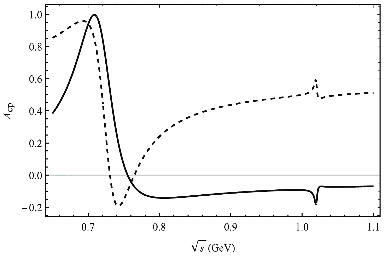
Figure 1. Plot of
$ A_{CP} $ as a function of$ \sqrt{s} $ corresponding to the central parameter values of the CKM matrix elements. The solid (dashed) line corresponds to the decay channel$ B^{0}\rightarrow \pi^+\pi^{-}\eta $ ($ B^{0}\rightarrow \pi^+\pi^{-}\eta' $ ).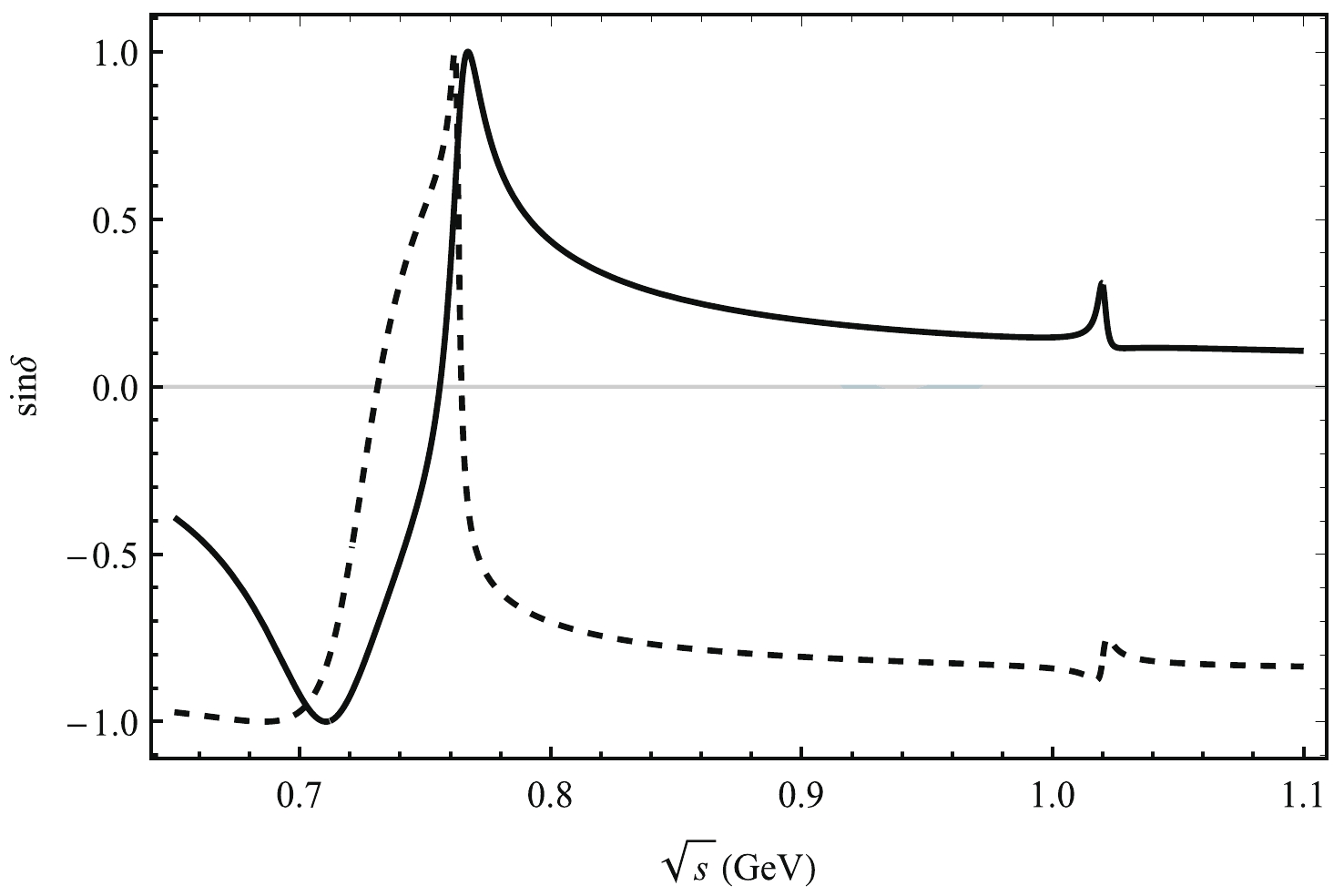
Figure 2. Plot of
$ {{\rm{sin}}}\delta $ as a function of$ \sqrt{s} $ corresponding to the central parameter values of the CKM matrix elements. The solid (dashed) line corresponds to the decay channel$ B^{0}\rightarrow \pi^+\pi^{-}\eta $ ($ B^{0}\rightarrow \pi^+\pi^{-}\eta' $ ).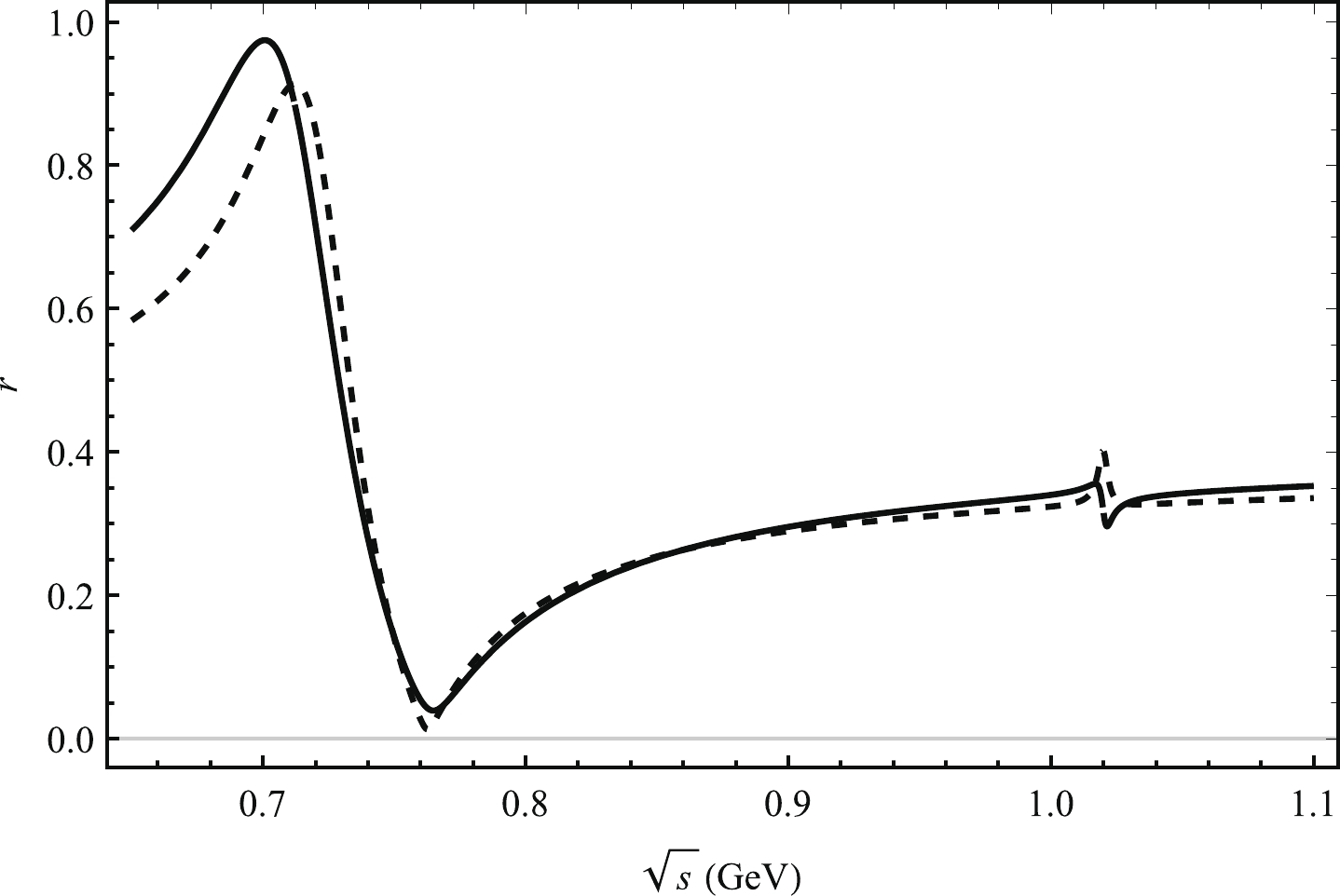
Figure 3. Plot of
$ r $ as a function of$ \sqrt{s} $ corresponding to the central parameter values of the CKM matrix elements. The solid (dashed) line corresponds to the decay channel$ B^{0}\rightarrow \pi^+\pi^{-}\eta $ ($ B^{0}\rightarrow \pi^+\pi^{-}\eta' $ ).We find that
$ CP $ violation is affected by the weak phase difference, strong phase difference, and$ r $ . The weak phase depends on the CKM matrix elements, which have little effect on our results. Hence, we present the results corresponding to the central parameter values of the CKM matrix elements. In Fig. 2, we present a plot of$ {{\rm{sin}}}\delta $ as a function of$ \sqrt{s} $ from the central parameter values$ \rho $ ,$ \eta $ ,$ \lambda $ , and$ A $ of the CKM matrix elements. We find that$ {{\rm{sin}}}\delta $ oscillates considerably in the area of$ \omega $ resonance and changes slightly in the area of$ \phi $ resonance. A plot of$ r $ as a function of$ \sqrt{s} $ is presented in Fig. 3.$ r $ changes sharply for the$ \omega $ resonance range and slightly for the$ \phi $ resonance range. -
In this paper, we introduce the formalism for
$ \rho-\omega-\phi $ meson interferences from isospin symmetry breaking. A new strong phase can be produced by the resonance contributions of$ \rho-\omega $ ,$ \rho-\phi $ , and$ \omega-\phi $ . The mechanism is applied to the decay process$ B^{0}\rightarrow \pi^+\pi^{-}\eta^{(')} $ . It is found that$ CP $ asymmetry oscillates greatly in the resonance range. The maximum$ CP $ asymmetry can reach$ 99.6 $ % and$ -18.2 $ % in the vicinity of the$ \omega $ resonance range and the$ \phi $ resonance range of the decay process$ B^{0}\rightarrow \pi^+\pi^{-}\eta $ , respectively. For the decay process$ B^{0}\rightarrow \pi^+\pi^{-}\eta' $ , the maximum$ CP $ asymmetry is$ 95.9 $ % and$ 59.5 $ % in the area of$ \omega $ resonance and$ \phi $ resonance, respectively. Our formalism can be used to calculate other decay process.Detection of the
$ CP $ violation signal is important in the$ B $ -meson decay process. For three body final states,$ CP $ violation is often dominated by quasi-two-body decay channels and depends on the relative phase between two quasi-two-body amplitudes. The numbers required to observe large$ CP $ violation depend on both the magnitudes of$ CP $ violation and the branching ratios of heavy$ B $ -meson decays. We find that the contribution of three meson mixing has little effect on the branching ratio and can be ignored safely because the mechanism can only provide the strong phase. For a one (three) standard deviation signature, the number of required$ B\bar{B} $ pairs is [54–56]$ N_{B\bar{B}}\sim \frac{1}{BRA_{CP}^{2}}(1-A_{CP}^{2})\Bigg(\frac{9}{BR A_{CP}^{2}}(1-A_{CP}^{2})\Bigg), $

(64) where BR is the branching ratio for
$ B\rightarrow \rho^{0}\eta^{(')} $ . We present the number of$ B\bar{B} $ pairs used to observe large$ CP $ violation at the LHC. For the channel$ B^{0}\rightarrow \rho^{0}(\omega,\phi)\eta\rightarrow \pi^{+}\pi^{-} \eta $ , the number of$ B\bar{B} $ pairs is$ 10^{4} $ ($ 10^{5} $ ) and$ 10^{8} $ ($ 10^{9} $ ) in the resonance ranges of$ \omega $ and$ \phi $ for a$ 1\sigma $ ($ 3\sigma $ ) signature. We need$ 10^{5} $ ($ 10^{6} $ ) and$ 10^{7} $ ($ 10^{8} $ )$ B\bar{B} $ pairs to observe$ CP $ violation from the two resonance ranges in the decay process$ B^{0}\rightarrow \rho^{0}(\omega,\phi)\eta^{'}\rightarrow \pi^{+}\pi^{-} \eta^{'} $ for a$ 1\sigma $ ($ 3\sigma $ ) signature, respectively.In the heavy-quark limit, strong-interaction corrections can be calculated at the leading power of
$ \Lambda_{\rm QCD}/m_{b} $ in QCD factorization [57]. The decay amplitudes can be expressed in terms of form factors and meson light-cone distribution amplitudes, including the nonfactorizable and chirally enhanced hard-scattering spectator and annihilation contributions at next-to-leading order in$ \alpha_{s} $ . In the leading order of the expansion of$ 1/m_{b} $ , hadronic matrix elements can be presented using the factorization approach. However, power counting is significantly different from the hard kernels due to transverse momenta between QCD factorization and perturbative QCD. The strong phases associated with hadronic matrix elements may be different for different factorization approaches. Hence, the result of CP violation can be affected by the different factorization approaches for our mixing mechanism.In 2010, the Large Hadron Collider (LHC) operated successfully for proton-proton collisions with a 7 TeV center-of-mass energy at CERN. With the designed center-of-mass energy of
$ 14 $ TeV and luminosity$ L=10^{34} {\rm cm}^{-2}{\rm s}^{-1} $ , the LHC provides new possibilities of searching for$ CP $ violation and new physics. The$ b\bar{b} $ production cross section is of the order of 0.5 mb, providing as many as$ 0.5\times 10^{12} $ bottom events per year at the LHC [58, 59]. The LHC can provide approximately$ 10^{13} $ $ B\bar{B} $ pairs. In particular, the LHCb detector is designed to study$ CP $ violation and rare decays in$ b $ -hadron systems precisely using a large number of$ b $ -hadrons produced at the LHC. Direct$ CP $ violation can be observed in the decay processes of$ B $ and$ \bar{B} $ to obtain differences from that of the LHCb detector. Furthermore, the ATLAS and CMS experiments are expected to discover new physics and focus on their$ B $ physics programs within the first few years [58, 59]. To extend its discovery potential, the LHC recently made a significant upgrade and increased its luminosity by a factor of five beyond its design value. As a result, it is possible to observe large$ CP $ violation in small energy ranges of the$ \rho^{0}\sim \omega $ and$ \rho^{0}\sim \phi $ resonances at the peak values of$ CP $ violation from LHC experiment at the high luminosity LHC (HL-LHC), even though the branching fractions in these regions may be small. For the experiments, it is possible to reconstruct$ \pi^{+} $ ,$ \pi^{-} $ , and$ \eta^{(')} $ mesons when the invariant masses of$ \pi^{+}\pi^{-} $ pairs are in the vicinity of the$ \omega $ or$ \phi $ resonances. Therefore, it is possible to observe large$ CP $ violation in$ B^{0}\rightarrow \rho^{0}(\omega,\phi)\eta^{(')}\rightarrow \pi^{+}\pi^{-} \eta^{(')} $ at the LHC. -
Functions related to the tree and penguin contributions are presented using the PQCD approach [43, 44, 60].
The hard scales
$ t $ are chosen as$ \begin{array}{l} t_e^1 = \rm{max}\{{\sqrt{x_3}m_{B},1/b_1,1/b_3}\}, \end{array} \tag{A1}$

$ \begin{array}{l} t_e^2 = \rm{max}\{{\sqrt{x_1}m_{B},1/b_1,1/b_3}\}, \end{array} \tag{A2}$

$ \begin{array}{l} t_f = \rm{max}\{\sqrt{x_1x_3}m_{B},\sqrt{(x_1-x_2)x_3}m_{B},1/b_1,1/b_2\}, \end{array} \tag{A3}$

$ \begin{array}{l} t_f^1 = \rm{max}\{{\sqrt{x_2x_3}m_{B},1/b_1,1/b_2}\}, \end{array} \tag{A4}$

$ \begin{array}{l} t_f^2 = \rm{max}\{{\sqrt{x_2x_3}m_{B},\sqrt{x_2+x_3-x_2x_3}m_{B},1/b_1,1/b_2}\}, \end{array} \tag{A5}$

$ \begin{aligned}[b] t_f^3 =& \rm{max}\{\sqrt{x_1+x_2+x_3-x_1x_3-x_2x_3}m_{B},\\&\sqrt{x_2x_3}m_{B},1/b_1,1/b_2\}, \end{aligned} \tag{A6}$

$ \begin{array}{l} t_f^4 = \rm{max}\{\sqrt{x_2x_3}m_{B},\sqrt{(x_1-x_2)x_3}m_{B},1/b_1,1/b_2\}. \end{array} \tag{A7}$

The function
$ h $ originates from the Fourier transformations of the function$ H^{(0)} $ [61]. They are defined by$ \begin{aligned}[b] h_{e}\left(x_{1}, x_{3}, b_{1}, b_{3}\right)=& K_{0}\left(\sqrt { x _ { 1 } x _ { 3 } } m _ { B } b _ { 1 } \left[\theta\left(b_{1}-b_{3}\right) K_{0}\left(\sqrt{x}_{3} m_{B} b_{1}\right) I_{0}\left(\sqrt{x}_{3} m_{B} b_{3}\right)\right.\right.\\ &\left.+\theta\left(b_{3}-b_{1}\right) K_{0}\left(\sqrt{x}_{3} m_{B} b_{3}\right) I_{0}\left(\sqrt{x}_{3} m_{B} b_{1}\right)\right] S_{t}\left(x_{3}\right), \end{aligned} \tag{A8}$ 
$ \begin{aligned}[b] h_{e}^{1}\left(x_{1}, x_{2}, b_{1}, b_{2}\right)=& K_{0}\left(\sqrt { x _ { 1 } x _ { 2 } } m _ { B } b _ { 1 } \left[\theta\left(b_{1}-b_{2}\right) K_{0}\left(\sqrt{x}_{2} m_{B} b_{1}\right) I_{0}\left(\sqrt{x}_{2} m_{B} b_{2}\right)\right.\right.\\& \left.+\theta\left(b_{2}-b_{1}\right) K_{0}\left(\sqrt{x}_{2} m_{B} b_{2}\right) I_{0}\left(\sqrt{x}_{2} m_{B} b_{1}\right)\right], \end{aligned}\tag{A9} $

$ \begin{aligned}[b] h_{f}\left(x_{1}, x_{2}, x_{3}, b_{1}, b_{2}\right)=&\left[\theta\left(b_{2}-b_{1}\right) I_{0}\left(M_{B} \sqrt{x_{1} x_{3}} b_{1}\right) K_{0}\left(M_{B} \sqrt{x_{1} x_{3}} b_{2}\right)\right.\\ &\left.+\left(b_{1} \longleftrightarrow b_{2}\right)\right] \cdot\left\{\begin{array}{ll} K_{0}\left(M_{B} F_{(1)} b_{2}\right), {\rm { for }}\; F_{(1)}^{2}>0 \\ \dfrac{{\rm i} \pi}{2} H_{0}^{(1)}\left(M_{B} \sqrt{\left.\left|F_{(1)^{2}}\right| b_{2}\right),}\right. {\rm { for }}\; F_{(1)}^{2}<0 \end{array},\right. \end{aligned}\tag{A10} $

$ \begin{aligned}[b] h_{f}^{1}\left(x_{1}, x_{2}, x_{3}, b_{1}, b_{2}\right)=& K_{0}\left(-{\rm i} \sqrt{x_{2} x_{3}} m_{B} b_{1}\left[\theta\left(b_{1}-b_{2}\right) K_{0}\left(-{\rm i} \sqrt{x}_{2} x_{3} m_{B} b_{1}\right) J_{0}\left(\sqrt{x}_{2} x_{3} m_{B} b_{2}\right)\right.\right.\\ &\left.+\theta\left(b_{2}-b_{1}\right) K_{0}\left(-{\rm i} \sqrt{x}_{2} x_{3} m_{B} b_{2}\right) J_{0}\left(\sqrt{x}_{2} x_{3} m_{B} b_{3}\right)\right], \end{aligned} \tag{A11}$

$ \begin{aligned}[b] h_{f}^{2}\left(x_{1}, x_{2}, x_{3}, b_{1}, b_{2}\right)=& K_{0}\left({\rm i} \sqrt { x _ { 2 } + x _ { 3 } - x _ { 2 } x _ { 3 } } m _ { B } b _ { 1 } \left[\theta\left(b_{1}-b_{2}\right) K_{0}\left(-{\rm i} \sqrt{x}_{2} x_{3} m_{B} b_{1}\right) J_{0}\left(\sqrt{x}_{2} x_{3} m_{B} b_{2}\right)\right.\right.\\ &\left.+\theta\left(b_{2}-b_{1}\right) K_{0}\left(-{\rm i} \sqrt{x}_{2} x_{3} m_{B} b_{2}\right) J_{0}\left(\sqrt{x}_{2} x_{3} m_{B} b_{1}\right)\right], \end{aligned} \tag{A12}$

$ \begin{aligned}[b] h_{f}^{3}\left(x_{1}, x_{2}, x_{3}, b_{1}, b_{2}\right)=&\left[\theta\left(b_{1}-b_{2}\right) K_{0}\left({\rm i} \sqrt{x_{2} x_{3}} b_{1} M_{B}\right) I_{0}\left({\rm i} \sqrt{x_{2} x_{3}} b_{2} M_{B}\right)\right.\\ &\left.+\left(b_{1} \longleftrightarrow b_{2}\right)\right] \cdot K_{0}\left(\sqrt{x_{1}+x_{2}+x_{3}-x_{1} x_{3}-x_{2} x_{3}} b_{1} M_{B}\right), \end{aligned}\tag{A13} $

$ \begin{aligned}[b] h_{f}^{4}\left(x_{1}, x_{2}, x_{3}, b_{1}, b_{2}\right)=&\left[\theta\left(b_{1}-b_{2}\right) K_{0}\left({\rm i} \sqrt{x_{2} x_{3}} b_{1} M_{B}\right) I_{0}\left({\rm i} \sqrt{x_{2} x_{3}} b_{2} M_{B}\right)\right.\\& \left.+\left(b_{1} \longleftrightarrow b_{2}\right)\right] \cdot\left\{\begin{array}{ll} K_{0}\left(M_{B} F_{(2)} b_{2}\right), {\rm { for }}\; F_{(2)}^{2}>0 \\ \dfrac{{\rm i} \pi}{2} H_{0}^{(1)}\left(M_{B} \sqrt{\left|F_{(2)^{2}}\right|} b_{2}\right), {\rm { for }}\; F_{(2)}^{2}<0 \end{array},\right. \end{aligned}\tag{A14} $

where
$ J_0 $ is the Bessel function,$ K_0 $ and$ I_0 $ are the modified Bessel functions$K_0(-{\rm i}x) = -\dfrac{\pi}{2}\mathrm{y}_0(x) + {\rm i}\,\dfrac{\pi}{2} {J}_0(x)$ , and$ F_{(j)} $ are defined by$ F_{(1)}^2=(x_1-x_2)x_3, \;\;\;\; F_{(2)}^2=(x_1-x_2)x_3. \tag{A15} $

The
$ S_t $ re-sums the threshold logarithms$ \ln^2x $ appearing in the hard kernels to all orders and is parameterized as$ S_t(x)=\frac{2^{1+2c}\Gamma(3/2+c)}{\sqrt \pi \Gamma(1+c)}[x(1-x)]^c, \tag{A16} $

with
$ c=0.3 $ . In the nonfactorizable contributions,$ S_t(x) $ has a small numerical effect on the amplitude [62].The Sudakov exponents are defined as
$ S_{a b}(t)=s\left(x_{1} \frac{m_{B}}{\sqrt{2}}, b_{1}\right)+s\left(x_{3} \frac{m_{B}}{\sqrt{2}}, b_{3}\right)+s\left(\left(1-x_{3}\right) \frac{m_{B}}{\sqrt{2}}, b_{3}\right)-\frac{1}{\beta_{1}}\left[\ln \frac{\ln (t / \Lambda)}{-\ln \left(b_{1} \Lambda\right)}+\ln \frac{\ln (t / \Lambda)}{-\ln \left(b_{3} \Lambda\right)}\right], \tag{A17}$ 
$ \begin{aligned}[b] S_{c d}(t)=& s\left(x_{1} \frac{m_{B}}{\sqrt{2}}, b_{1}\right)+s\left(x_{2} \frac{m_{B}}{\sqrt{2}}, b_{2}\right)+s\left(\left(1-x_{2}\right) \frac{m_{B}}{\sqrt{2}}, b_{2}\right)+s\left(x_{3} \frac{m_{B}}{\sqrt{2}}, b_{1}\right)+s\left(\left(1-x_{3}\right) \frac{m_{B}}{\sqrt{2}}, b_{1}\right) \\& -\frac{1}{\beta_{1}}\left[\ln \frac{\ln (t / \Lambda)}{-\ln \left(b_{1} \Lambda\right)}+\ln \frac{\ln (t / \Lambda)}{-\ln \left(b_{2} \Lambda\right)}\right], \end{aligned} \tag{A18}$

$ \begin{aligned}[b] S_{e f}(t)=& s\left(x_{1} \frac{m_{B}}{\sqrt{2}}, b_{1}\right)+s\left(x_{2} \frac{m_{B}}{\sqrt{2}}, b_{2}\right)+s\left(\left(1-x_{2}\right) \frac{m_{B}}{\sqrt{2}}, b_{2}\right)+s\left(x_{3} \frac{m_{B}}{\sqrt{2}}, b_{2}\right)+s\left(\left(1-x_{3}\right) \frac{m_{B}}{\sqrt{2}}, b_{2}\right) \\& -\frac{1}{\beta_{1}}\left[\ln \frac{\ln (t / \Lambda)}{-\ln \left(b_{1} \Lambda\right)}+2 \ln \frac{\ln (t / \Lambda)}{-\ln \left(b_{2} \Lambda\right)}\right]. \end{aligned} \tag{A19}$

$ S_{gh}(t)=s\left( x_2\frac{m_B}{\sqrt{2}},b_2 \right) +s\left( x_3\frac{m_B}{\sqrt{2}},b_3 \right) +s\left( \left( 1-x_2 \right) \frac{m_B}{\sqrt{2}},b_2 \right) +s\left( \left( 1-x_3 \right) \frac{m_B}{\sqrt{2}},b_3 \right)-\frac{1}{\beta _1}\left[ \ln \frac{\ln\mathrm{(}t/\Lambda )}{-\ln \left( b_2\Lambda \right)}+2\ln \frac{\ln\mathrm{(}t/\Lambda )}{-\ln \left( b_3\Lambda \right)} \right] . \tag{A20} $

The explicit form of the function
$ s(k,b) $ is [44]$ s(k, b)= \frac{2}{3 \beta_{1}}\left[\hat{q} \ln \left(\frac{\hat{q}}{\hat{b}}-\hat{q}+\hat{b}\right)\right]+\frac{A^{(2)}}{4 \beta_{1}^{2}}\left(\frac{\hat{q}}{\hat{b}}-1\right) -\left[\frac{A^{(2)}}{4 \beta_{1}^{2}}-\frac{1}{3 \beta_{1}}\left(2 \gamma_{E}-1-\ln 2\right)\right] \ln \left(\frac{\hat{q}}{\hat{b}}\right), \tag{A21}$

where the variables are defined by
$ \hat q\equiv \rm{ln}[k/(\sqrt \Lambda)],\quad \hat b\equiv \rm{ln}[1/(b\Lambda)], \tag{A22}$

and the coefficients
$ A^{(i)} $ and$ \beta_i $ are$ A^{(2)} = \frac{67}{9} -\frac{\pi^2}{3}-\frac{10}{27}n_f+\frac{8}{3}\beta_1\rm{ln}\left(\frac{1}{2}{\rm e}^{\gamma_E}\right), \tag{A23}$

$ \beta_1 = \frac{33-2n_f}{12},\tag{A24}$

where
$ n_f $ is the number of quark flavors, and$ \gamma_E $ is the Euler constant.The decay amplitudes
$ F_{e} $ ,$ F_{e \rho} $ , and$ F_{e \omega} $ induced by inserting the$ (V-A)(V-A) $ operators are [63]$ \begin{aligned}[b] F_{e}=& 4 \sqrt{2} \pi G_{F} C_{F} f_{\rho} m_{B}^{4} \int_{0}^{1} {\rm d} x_{1} {\rm d} x_{3} \int_{0}^{\infty} b_{1} {\rm d} b_{1} b_{3} {\rm d} b_{3} \phi_{B}\left(x_{1}, b_{1}\right) \cdot\left\{\left[\left(1+x_{3}\right) \phi_{\eta}^{A}\left(x_{3}, b_{3}\right)+r_{\eta}\left(1-2 x_{3}\right)\left(\phi_{\eta}^{P}\left(x_{3}, b_{3}\right)\right.\right.\right.\\& \left.\left.\left.+\phi_{\eta}^{T}\left(x_{3}, b_{3}\right)\right)\right] \cdot \alpha_{s}\left(t_{e}^{1}\right) h_{e}\left(x_{1}, x_{3}, b_{1}, b_{3}\right) \exp \left[-S_{a b}\left(t_{e}^{1}\right)\right]+2 r_{\eta} \phi_{\eta}^{P}\left(x_{3}, b_{3}\right) \alpha_{s}\left(t_{e}^{2}\right) h_{e}\left(x_{3}, x_{1}, b_{3}, b_{1}\right) \exp \left[-S_{a b}\left(t_{e}^{2}\right)\right]\right\}, \end{aligned} \tag{A25}$

$ \begin{aligned}[b] F_{e \rho}=& 4 \sqrt{2} G_{F} \pi C_{F} m_{B}^{4} \int_{0}^{1} {\rm d} x_{1} {\rm d} x_{3} \int_{0}^{\infty} b_{1} {\rm d} b_{1} b_{3} {\rm d} b_{3} \phi_{B}\left(x_{1}, b_{1}\right) \cdot\left\{\left[\left(1+x_{3}\right) \phi_{\rho}\left(x_{3}, b_{3}\right)+\left(1-2 x_{3}\right) r_{\rho}\left(\phi_{\rho}^{s}\left(x_{3}, b_{3}\right)\right.\right.\right.\\& \left.\left.\left.+\phi_{\rho}^{t}\left(x_{3}, b_{3}\right)\right)\right] \alpha_{s}\left(t_{e}^{1}\right) h_{e}\left(x_{1}, x_{3}, b_{1}, b_{3}\right) \exp \left[-S_{a b}\left(t_{e}^{1}\right)\right]+2 r_{\rho} \phi_{\rho}^{s}\left(x_{3}, b_{3}\right) \alpha_{s}\left(t_{e}^{2}\right) h_{e}\left(x_{3}, x_{1}, b_{3}, b_{1}\right) \exp \left[-S_{a b}\left(t_{e}^{2}\right)\right]\right\}, \end{aligned}\tag{A26} $

$ \begin{aligned}[b] F_{e \omega}=& 4 \sqrt{2} G_{F} \pi C_{F} m_{B}^{4} \int_{0}^{1} {\rm d} x_{1} {\rm d} x_{3} \int_{0}^{\infty} b_{1} {\rm d} b_{1} b_{3} {\rm d} b_{3} \phi_{B}\left(x_{1}, b_{1}\right)\left\{\left[\left(1+x_{3}\right) \phi_{\omega}\left(x_{3}, b_{3}\right)+\left(1-2 x_{3}\right) r_{\omega}\left(\phi_{\omega}^{s}\left(x_{3}, b_{3}\right)\right.\right.\right.\\& \left.\left.\left.+\phi_{\omega}^{t}\left(x_{3}, b_{3}\right)\right)\right] \alpha_{s}\left(t_{e}^{1}\right) h_{e}\left(x_{1}, x_{3}, b_{1}, b_{3}\right) \exp \left[-S_{a b}\left(t_{e}^{1}\right)\right]+2 r_{\omega} \phi_{\omega}^{s}\left(x_{3}, b_{3}\right) \alpha_{s}\left(t_{e}^{2}\right) h_{e}\left(x_{3}, x_{1}, b_{3}, b_{1}\right) \exp \left[-S_{a b}\left(t_{e}^{2}\right)\right]\right\}. \end{aligned}\tag{A27} $

where the color factor
$ C_F=\dfrac{3}{4} $ ,$ \phi _B $ and$ \phi _{\eta}^{A,T,P} $ are the light cone distribution amplitudes (LCDAs) of the heavy B meson and light$ \eta $ meson, and$ r_{\eta}\equiv r_{\pi} = m^{\pi}_{0}/m_{B} $ . The functions$ h_e $ , scales$ t_{e}^{i} $ , and Sudakov factors are explicitly provided.We may obtain the
$ (S+P)(S-P) $ operators from the$ (V-A)(V-A) $ operators. Because neither the scalar nor pseudoscalar density give a contribution to vector meson production, we obtain the$ (S+P)(S-P) $ operators, and we can get$ F_{e}^{P2}=0 $ .$ \begin{aligned}[b]F_{e \rho}^{P}=& 8 \sqrt{2} G_{F} \pi C_{F} f_{\eta}^{d} m_{B}^{4} \int_{0}^{1} {\rm d} x_{1} {\rm d} x_{3} \int_{0}^{\infty} b_{1} {\rm d} b_{1} b_{3} {\rm d} b_{3} \phi_{B}\left(x_{1}, b_{1}\right) \cdot\left\{\left[\phi_{\rho}\left(x_{3}, b_{3}\right)+r_{\rho}\left(\left(x_{3}+2\right) \phi_{\rho}^{s}\left(x_{3}, b_{3}\right)-x_{3} \phi_{\rho}^{t}\left(x_{3}, b_{3}\right)\right)\right]\right.\\& \left.\cdot \alpha_{s}\left(t_{e}^{1}\right) h_{e}\left(x_{1}, x_{3}, b_{1}, b_{3}\right) \exp \left[-S_{a b}\left(t_{e}^{1}\right)\right]+\left(x_{1} \phi_{\rho}\left(x_{3}, b_{3}\right)+2 r_{\rho} \phi_{\rho}^{s}\left(x_{3}, b_{3}\right)\right) \alpha_{s}\left(t_{e}^{2}\right) h_{e}\left(x_{3}, x_{1}, b_{3}, b_{1}\right) \exp \left[-S_{a b}\left(t_{e}^{2}\right)\right]\right\}, \end{aligned}\tag{A28} $

$ \begin{aligned}[b] F_{e \omega}^{P 2}=& 8 \sqrt{2} G_{F} \pi C_{F} r_{\eta} m_{B}^{4} \int_{0}^{1} {\rm d} x_{1} {\rm d} x_{3} \int_{0}^{\infty} b_{1} {\rm d} b_{1} b_{3} {\rm d} b_{3} \phi_{B}\left(x_{1}, b_{1}\right)\left\{\left[\phi_{\omega}\left(x_{3}, b_{3}\right)+r_{\omega}\left(\left(x_{3}+2\right) \phi_{\omega}^{s}\left(x_{3}, b_{3}\right)-x_{3} \phi_{\omega}^{t}\left(x_{3}, b_{3}\right)\right)\right]\right.\\ &\left.\times \alpha_{s}\left(t_{e}^{1}\right) h_{e}\left(x_{1}, x_{3}, b_{1}, b_{3}\right) \exp \left[-S_{a b}\left(t_{e}^{1}\right)\right]+\left(x_{1} \phi_{\omega}\left(x_{3}, b_{3}\right)+2 r_{\omega} \phi_{\omega}^{s}\left(x_{3}, b_{3}\right)\right) \alpha_{s}\left(t_{e}^{2}\right) h_{e}\left(x_{3}, x_{1}, b_{3}, b_{1}\right) \exp \left[-S_{a b}\left(t_{e}^{2}\right)\right]\right\}. \end{aligned}\tag{A29} $

The decay amplitude of the
$ (V-A)(V-A) $ and$ (V-A)(V+A) $ operators can be written as follows:$ \begin{aligned}[b] M_{e}=&-M_{e}^{P 2}=\frac{16}{\sqrt{3}} G_{F} \pi C_{F} m_{B}^{4} \int_{0}^{1} {\rm d} x_{1} {\rm d} x_{2} {\rm d} x_{3} \int_{0}^{\infty} b_{1} {\rm d} b_{1} b_{2} {\rm d} b_{2} \phi_{B}\left(x_{1}, b_{1}\right) \phi_{\omega}\left(x_{2}, b_{2}\right) \\& \times\left\{\left[2 x_{3} r_{\eta} \phi_{\eta}^{T}\left(x_{3}, b_{1}\right)-x_{3} \phi_{\eta}^{A}\left(x_{3}, b_{1}\right)\right] \alpha_{s}\left(t_{f}\right) h_{f}\left(x_{1}, x_{2}, x_{3}, b_{1}, b_{2}\right) \exp \left[-S_{c d}\left(t_{f}\right)\right]\right\}, \end{aligned}\tag{A30} $

$ \begin{aligned}[b] M_{e}^{P}=&-\frac{32}{\sqrt{3}} G_{F} \pi C_{F} r_{\rho} m_{B}^{4} \int_{0}^{1} {\rm d} x_{1} {\rm d} x_{2} {\rm d} x_{3} \int_{0}^{\infty} b_{1} {\rm d} b_{1} b_{2} {\rm d} b_{2} \phi_{B}\left(x_{1}, b_{1}\right) \cdot\left\{\left[x_{2} \phi_{\eta}^{A}\left(x_{3}, b_{2}\right)\left(\phi_{\rho}^{s}\left(x_{2}, b_{2}\right)-\phi_{\rho}^{t}\left(x_{2}, b_{2}\right)\right)\right.\right.\\& +r_{\eta}\left(\left(x_{2}+x_{3}\right)\left(\phi_{\eta}^{P}\left(x_{3}, b_{2}\right) \cdot \phi_{\rho}^{s}\left(x_{2}, b_{2}\right)+\phi_{\eta}^{T}\left(x_{3}, b_{2}\right) \phi_{\rho}^{t}\left(x_{2}, b_{2}\right)\right)+\left(x_{3}-x_{2}\right)\left(\phi_{\eta}^{P}\left(x_{3}, b_{2}\right) \phi_{\rho}^{t}\left(x_{2}, b_{2}\right)\right.\right.\\& \left.\left.\left.\left.+\phi_{\eta}^{T}\left(x_{3}, b_{2}\right) \phi_{\rho}^{s}\left(x_{2}, b_{2}\right)\right)\right)\right] \alpha_{s}\left(t_{f}\right) h_{f}\left(x_{1}, x_{2}, x_{3}, b_{1}, b_{2}\right) \exp \left[-S_{c d}\left(t_{f}\right)\right]\right\}, \end{aligned}\tag{A31} $

$ \begin{aligned}[b] M_{e}^{P 1}=&-\frac{32}{\sqrt{3}} G_{F} \pi C_{F} r_{\omega} m_{B}^{4} \int_{0}^{1} {\rm d} x_{1} {\rm d} x_{2} {\rm d} x_{3} \int_{0}^{\infty} b_{1} {\rm d} b_{1} b_{2} {\rm d} b_{2} \phi_{B}\left(x_{1}, b_{1}\right)\left\{\left[x_{2} \phi_{\eta}^{A}\left(x_{3}, b_{1}\right)\left(\phi_{\omega}^{s}\left(x_{2}, b_{2}\right)-\phi_{\omega}^{t}\left(x_{2}, b_{2}\right)\right)\right.\right.\\& +r_{\eta}\left(\left(x_{2}+x_{3}\right)\left(\phi_{\eta}^{p}\left(x_{3}, b_{1}\right) \phi_{\omega}^{s}\left(x_{2}, b_{2}\right)+\phi_{\eta}^{T}\left(x_{3}, b_{1}\right) \phi_{\omega}^{t}\left(x_{2}, b_{2}\right)\right)+\left(x_{3}-x_{2}\right)\left(\phi_{\eta}^{P}\left(x_{3}, b_{1}\right) \phi_{\omega}^{t}\left(x_{2}, b_{2}\right)\right.\right.\\& \left.\left.\left.\left. +\phi_{\eta}^{T}\left(x_{3}, b_{1}\right) \phi_{\omega}^{s}\left(x_{2}, b_{2}\right)\right)\right)\right] \alpha_{s}\left(t_{f}\right) h_{f}\left(x_{1}, x_{2}, x_{3}, b_{1}, b_{2}\right) \exp \left[-S_{c d}\left(t_{f}\right)\right]\right\}. \end{aligned}\tag{A32} $

For the nonfactorizable annihilation diagrams, there are three types of decay amplitudes. For the
$ (V-A)(V-A) $ operators, the decay amplitude$ M_a $ is$ \begin{aligned}[b] M_{a}=& \frac{16}{\sqrt{3}} \pi G_{F} C_{F} m_{B}^{4} \int_{0}^{1} {\rm d} x_{1} {\rm d} x_{2} {\rm d} x_{3} \int_{0}^{\infty} b_{1} {\rm d} b_{1} b_{2} {\rm d} b_{2} \phi_{B}\left(x_{1}, b_{1}\right) \\& \times\left\{\left[r_{\omega} r_{\eta}\left(x_{3}-x_{2}\right)\left[\phi_{\eta}^{P}\left(x_{3}, b_{2}\right) \phi_{\omega}^{t}\left(x_{2}, b_{2}\right)+\phi_{\eta}^{T}\left(x_{3}, b_{2}\right) \phi_{\omega}^{s}\left(x_{2}, b_{2}\right)\right]+r_{\omega} r_{\eta}\left(x_{2}+x_{3}\right)\right.\right.\\& \left.\times\left[\phi_{\eta}^{P}\left(x_{3}, b_{2}\right) \phi_{\omega}^{s}\left(x_{2}, b_{2}\right)+\phi_{\eta}^{T}\left(x_{3}, b_{2}\right) \phi_{\omega}^{t}\left(x_{2}, b_{2}\right)\right]+x_{3} \phi_{\omega}\left(x_{2}, b_{2}\right) \phi_{\eta}^{A}\left(x_{3}, b_{2}\right)\right] \alpha_{s}\left(t_{f}^{4}\right) h_{f}^{4}\left(x_{1}, x_{2}, x_{3}, b_{1}, b_{2}\right) \\ & \times \exp \left[-S_{e f}\left(t_{f}^{4}\right)\right]-\left[r_{\omega} r_{\eta}\left(x_{2}-x_{3}\right)\left[\phi_{\eta}^{P}\left(x_{3}, b_{2}\right) \phi_{\omega}^{t}\left(x_{2}, b_{2}\right)+\phi_{\eta}^{T}\left(x_{3}, b_{2}\right) \phi_{\omega}^{s}\left(x_{2}, b_{2}\right)\right]\right.\\& \left.+r_{\omega} r_{\eta}\left[\left(2+x_{2}+x_{3}\right) \phi_{\eta}^{P}\left(x_{3}, b_{2}\right) \phi_{\omega}^{s}\left(x_{2}, b_{2}\right)-\left(2-x_{2}-x_{3}\right) \phi_{\eta}^{T}\left(x_{3}, b_{2}\right) \phi_{\omega}^{t}\left(x_{2}, b_{2}\right)\right]+x_{2} \phi_{\omega}\left(x_{2}, b_{2}\right) \phi_{\eta}^{A}\left(x_{3}, b_{2}\right)\right] \\& \left.\times \alpha_{s}\left(t_{f}^{3}\right) h_{f}^{3}\left(x_{1}, x_{2}, x_{3}, b_{1}, b_{2}\right) \exp \left[-S_{e f}\left(t_{f}^{3}\right)\right]\right\}. \end{aligned}\tag{A33} $

For the
$ (V-A)(V-A) $ and$ (S-P)(S+P) $ operators, we have$ \begin{aligned}[b] M_{a}^{P 1}= &\frac{16}{\sqrt{3}} G_{F} \pi C_{F} m_{B}^{4} \int_{0}^{1} {\rm d} x_{1} {\rm d} x_{2} {\rm d} x_{3} \int_{0}^{\infty} b_{1} {\rm d} b_{1} b_{2} {\rm d} b_{2} \phi_{B}\left(x_{1}, b_{1}\right)\left\{\left[x_{2} r_{\omega} \phi_{\eta}^{A}\left(x_{3}, b_{2}\right)\left(\phi_{\omega}^{s}\left(x_{2}, b_{2}\right)+\phi_{\omega}^{t}\left(x_{2}, b_{2}\right)\right)\right.\right.\\& \left.-x_{3} r_{\eta}\left(\phi_{\eta}^{P}\left(x_{3}, b_{2}\right)+\phi_{\eta}^{T}\left(x_{3}, b_{2}\right)\right) \phi_{\omega}\left(x_{2}, b_{2}\right)\right] \alpha_{s}\left(t_{f}^{4}\right) h_{f}^{4}\left(x_{1}, x_{2}, x_{3}, b_{1}, b_{2}\right) \exp \left[-S_{e f}\left(t_{f}^{4}\right)\right] \\& +\left[\left(2-x_{2}\right) r_{\omega} \phi_{\eta}^{A}\left(x_{3}, b_{2}\right)\left(\phi_{\omega}^{s}\left(x_{2}, b_{2}\right)+\phi_{\omega}^{t}\left(x_{2}, b_{2}\right)\right)-\left(2-x_{3}\right) r_{\eta}\left(\phi_{\eta}^{P}\left(x_{3}, b_{2}\right)+\phi_{\eta}^{T}\left(x_{3}, b_{2}\right)\right) \phi_{\omega}\left(x_{2}, b_{2}\right)\right] \\& \left.\times \alpha_{s}\left(t_{f}^{3}\right) h_{f}^{3}\left(x_{1}, x_{2}, x_{3}, b_{1}, b_{2}\right) \exp \left[-S_{e f}\left(t_{f}^{3}\right)\right]\right\}, \end{aligned}\tag{A34} $

$ \begin{aligned}[b] M_{a}^{P 2}=&-\frac{16}{\sqrt{3}} \pi G_{F} C_{F} m_{B}^{4} \int_{0}^{1} {\rm d} x_{1} {\rm d} x_{2} {\rm d} x_{3} \int_{0}^{\infty} b_{1} {\rm d} b_{1} b_{2} {\rm d} b_{2} \phi_{B}\left(x_{1}, b_{1}\right)\left\{\left[x_{2} \phi_{\omega}\left(x_{2}, b_{2}\right) \phi_{\eta}^{A}\left(x_{3}, b_{2}\right)\right.\right.\\& +r_{\omega} r_{\eta}\left(\left(x_{2}-x_{3}\right)\left(\phi_{\eta}^{P}\left(x_{3}, b_{2}\right) \phi_{\omega}^{t}\left(x_{2}, b_{2}\right)+\phi_{\eta}^{T}\left(x_{3}, b_{2}\right) \phi_{\omega}^{s}\left(x_{2}, b_{2}\right)\right)+\left(x_{2}+x_{3}\right)\left(\phi_{\eta}^{P}\left(x_{3}, b_{2}\right) \phi_{\omega}^{s}\left(x_{2}, b_{2}\right)\right.\right.\\& \left.\left.\left.+\phi_{\eta}^{T}\left(x_{3}, b_{2}\right) \phi_{\omega}^{t}\left(x_{2}, b_{2}\right)\right)\right)\right] \alpha_{s}\left(t_{f}^{4}\right) h_{f}^{4}\left(x_{1}, x_{2}, x_{3}, b_{1}, b_{2}\right) \exp \left[-S_{e f}\left(t_{f}^{4}\right)\right]-\left[x_{3} \phi_{\omega}\left(x_{2}, b_{2}\right) \phi_{\eta}^{A}\left(x_{3}, b_{2}\right)\right.\\& +r_{\omega} r_{\eta}\left(\left(x_{3}-x_{2}\right)\left(\phi_{\eta}^{P}\left(x_{3}, b_{2}\right) \phi_{\omega}^{t}\left(x_{2}, b_{2}\right)+\phi_{\eta}^{T}\left(x_{3}, b_{2}\right) \phi_{\omega}^{s}\left(x_{2}, b_{2}\right)\right)+\left(2+x_{2}+x_{3}\right) \phi_{\eta}^{P}\left(x_{3}, b_{2}\right) \phi_{\omega}^{s}\left(x_{2}, b_{2}\right)\right.\\& \left.\left.\left.-\left(2-x_{2}-x_{3}\right) \phi_{\eta}^{T}\left(x_{3}, b_{2}\right) \phi_{\omega}^{t}\left(x_{2}, b_{2}\right)\right)\right] \alpha_{s}\left(t_{f}^{3}\right) h_{f}^{3}\left(x_{1}, x_{2}, x_{3}, b_{1}, b_{2}\right) \exp \left[-S_{e f}\left(t_{f}^{3}\right)\right]\right\}, \end{aligned}\tag{A35} $

For the nonfactorizable diagrams, the corresponding decay amplitudes are
$ \begin{aligned}[b] M_{e \rho}=&-\frac{16}{\sqrt{3}} G_{F} \pi C_{F} m_{B}^{4} \int_{0}^{1} {\rm d} x_{1} {\rm d} x_{2} {\rm d} x_{3} \int_{0}^{\infty} b_{1} {\rm d} b_{1} b_{2} {\rm d} b_{2} \phi_{B}\left(x_{1}, b_{1}\right) \phi_{\eta}^{A}\left(x_{2}, b_{2}\right) \\& \times\left\{x_{3}\left[\phi_{\rho}\left(x_{3}, b_{2}\right)-2 r_{\rho} \phi_{\rho}^{t}\left(x_{3}, b_{3}\right)\right] \alpha_{s}\left(t_{f}\right) h_{f}\left(x_{1}, x_{2}, x_{3}, b_{1}, b_{2}\right) \exp \left[-S_{c d}\left(t_{f}\right)\right]\right\}, \end{aligned}\tag{A36} $

$ \begin{aligned}[b] M_{e \omega}=&-\frac{16}{\sqrt{3}} G_{F} \pi C_{F} m_{B}^{4} \int_{0}^{1} {\rm d} x_{1} {\rm d} x_{2} {\rm d} x_{3} \int_{0}^{\infty} b_{1} {\rm d} b_{1} b_{2} {\rm d} b_{2} \phi_{B}\left(x_{1}, b_{1}\right) \phi_{\eta}^{A}\left(x_{2}, b_{2}\right) \\& \times\left\{x_{3}\left[\phi_{\omega}\left(x_{3}, b_{1}\right)-2 r_{\omega} \phi_{\omega}^{t}\left(x_{3}, b_{1}\right)\right] \alpha_{s}\left(t_{f}\right) h_{f}\left(x_{1}, x_{2}, x_{3}, b_{1}, b_{2}\right) \exp \left[-S_{c d}\left(t_{f}\right)\right]\right\}, \end{aligned}\tag{A37} $

and
$ M_{e\omega}^{P1}=0,\; \; \; \; \; \; \; \; \; \; \; \; \; \; \; \; \; M_{e\omega}^{P2}=M_{e\omega}. \tag{A38} $

For the nonfactorizable annihilation diagrams, all three wave functions are involved. The three types of decay amplitudes are of the form
$ \begin{aligned}[b] M_{a \omega}=& \frac{16}{\sqrt{3}} G_{F} \pi C_{F} m_{B}^{4} \int_{0}^{1} {\rm d} x_{1} {\rm d} x_{2} {\rm d} x_{3} \int_{0}^{\infty} b_{1} {\rm d} b_{1} b_{2} {\rm d} b_{2} \phi_{B}\left(x_{1}, b_{1}\right)\left\{\left[x_{3} \phi_{\omega}\left(x_{3}, b_{2}\right) \phi_{\eta}^{A}\left(x_{2}, b_{2}\right)\right.\right.\\ &+r_{\omega} r_{\eta}\left(\left(x_{3}-x_{2}\right)\left(\phi_{\eta}^{P}\left(x_{2}, b_{2}\right) \phi_{\omega}^{t}\left(x_{3}, b_{2}\right)+\phi_{\eta}^{T}\left(x_{2}, b_{2}\right) \phi_{\omega}^{s}\left(x_{3}, b_{2}\right)\right)+\left(x_{3}+x_{2}\right)\left(\phi_{\eta}^{P}\left(x_{2}, b_{2}\right) \phi_{\omega}^{s}\left(x_{3}, b_{2}\right)\right.\right.\\& \left.\left.+\phi_{\eta}^{T}\left(x_{2}, b_{2}\right) \phi_{\omega}^{t}\left(x_{3}, b_{2}\right)\right)\right] \alpha_{s}\left(t_{f}^{4}\right) h_{f}^{4}\left(x_{1}, x_{2}, x_{3}, b_{1}, b_{2}\right) \exp \left[-S_{e f}\left(t_{f}^{4}\right)\right]-\left[x_{2} \phi_{\omega}\left(x_{3}, b_{2}\right) \phi_{\eta}^{A}\left(x_{2}, b_{2}\right)\right.\\& +r_{\omega} r_{\eta}\left(\left(x_{2}-x_{3}\right)\left(\phi_{\eta}^{P}\left(x_{2}, b_{2}\right) \phi_{\omega}^{t}\left(x_{3}, b_{2}\right)+\phi_{\eta}^{T}\left(x_{2}, b_{2}\right) \phi_{\omega}^{s}\left(x_{3}, b_{2}\right)\right)+r_{\omega} r_{\eta}\left(\left(2+x_{2}+x_{3}\right) \phi_{\eta}^{P}\left(x_{2}, b_{2}\right) \phi_{\omega}^{s}\left(x_{3}, b_{2}\right)\right.\right.\\& \left.\left.\left.\left.-\left(2-x_{2}-x_{3}\right) \phi_{\eta}^{T}\left(x_{2}, b_{2}\right) \phi_{\omega}^{t}\left(x_{3}, b_{2}\right)\right)\right)\right] \alpha_{s}\left(t_{f}^{3}\right) h_{f}^{3}\left(x_{1}, x_{2}, x_{3}, b_{1}, b_{2}\right) \exp \left[-S_{e f}\left(t_{f}^{3}\right)\right]\right\}, \end{aligned}\tag{A39} $

$ \begin{aligned}[b] M_{a \omega}^{P 1}=&-\frac{16}{\sqrt{3}} G_{F} \pi C_{F} m_{B}^{4} \int_{0}^{1} {\rm d} x_{1} {\rm d} x_{2} {\rm d} x_{3} \int_{0}^{\infty} b_{1} {\rm d} b_{1} b_{2} {\rm d} b_{2} \phi_{B}\left(x_{1}, b_{1}\right)\left\{\left[x_{2} r_{\eta} \phi_{\omega}\left(x_{3}, b_{2}\right)\left(\phi_{\eta}^{P}\left(x_{2}, b_{2}\right)+\phi_{\eta}^{T}\left(x_{2}, b_{2}\right)\right)\right.\right.\\& \left.-x_{3} r_{\omega}\left(\phi_{\omega}^{s}\left(x_{3}, b_{2}\right)+\phi_{\omega}^{t}\left(x_{3}, b_{2}\right)\right) \phi_{\eta}^{A}\left(x_{2}, b_{2}\right)\right] \alpha_{s}\left(t_{f}^{4}\right) h_{f}^{4}\left(x_{1}, x_{2}, x_{3}, b_{1}, b_{2}\right) \exp \left[-S_{e f}\left(t_{f}^{4}\right)\right] \\& +\left[\left(2-x_{2}\right) r_{\eta} \phi_{\omega}\left(x_{3}, b_{2}\right)\left(\phi_{\eta}^{P}\left(x_{2}, b_{2}\right)+\phi_{\eta}^{T}\left(x_{2}, b_{2}\right)\right)-\left(2-x_{3}\right) r_{\omega}\left(\phi_{\omega}^{s}\left(x_{3}, b_{2}\right)+\phi_{\omega}^{t}\left(x_{3}, b_{2}\right)\right) \phi_{\eta}^{A}\left(x_{2}, b_{2}\right)\right] \\& \left.\times \alpha_{s}\left(t_{f}^{3}\right) h_{f}^{3}\left(x_{1}, x_{2}, x_{3}, b_{1}, b_{2}\right) \exp \left[-S_{e f}\left(t_{f}^{3}\right)\right]\right\}, \end{aligned}\tag{A40} $

$ \begin{aligned}[b] M_{a \omega}^{P 2}=&-\frac{16}{\sqrt{3}} \pi G_{F} C_{F} m_{B}^{4} \int_{0}^{1} {\rm d} x_{1} {\rm d} x_{2} {\rm d} x_{3} \int_{0}^{\infty} b_{1} {\rm d} b_{1} b_{2} {\rm d} b_{2} \phi_{B}\left(x_{1}, b_{1}\right)\left\{\left[x_{2} \phi_{\omega}\left(x_{3}, b_{2}\right) \phi_{\eta}^{A}\left(x_{2}, b_{2}\right)\right.\right.\\& +r_{\omega} r_{\eta}\left(\left(x_{2}-x_{3}\right)\left(\phi_{\eta}^{P}\left(x_{2}, b_{2}\right) \phi_{\omega}^{t}\left(x_{3}, b_{2}\right)+\phi_{\eta}^{T}\left(x_{2}, b_{2}\right) \phi_{\omega}^{s}\left(x_{3}, b_{2}\right)\right)+\left(x_{2}+x_{3}\right)\left(\phi_{\eta}^{P}\left(x_{2}, b_{2}\right) \phi_{\omega}^{s}\left(x_{3}, b_{2}\right)\right.\right.\\& \left.\left.\left.+\phi_{\eta}^{T}\left(x_{2}, b_{2}\right) \phi_{\omega}^{t}\left(x_{3}, b_{2}\right)\right)\right)\right] \alpha_{s}\left(t_{f}^{4}\right) h_{f}^{4}\left(x_{1}, x_{2}, x_{3}, b_{1}, b_{2}\right) \exp \left[-S_{e f}\left(t_{f}^{4}\right)\right]-\left[x_{3} \phi_{\omega}\left(x_{3}, b_{2}\right) \phi_{\eta}^{A}\left(x_{2}, b_{2}\right)\right.\\& +r_{\omega} r_{\eta}\left(\left(x_{3}-x_{2}\right)\left(\phi_{\eta}^{P}\left(x_{2}, b_{2}\right) \phi_{\omega}^{t}\left(x_{3}, b_{2}\right)+\phi_{\eta}^{T}\left(x_{2}, b_{2}\right) \phi_{\omega}^{s}\left(x_{3}, b_{2}\right)\right)+\left(2+x_{2}+x_{3}\right) \phi_{\eta}^{P}\left(x_{2}, b_{2}\right) \phi_{\omega}^{s}\left(x_{3}, b_{2}\right)\right.\\& \left.\left.\left.-\left(2-x_{2}-x_{3}\right) \phi_{\eta}^{T}\left(x_{2}, b_{2}\right) \phi_{\omega}^{t}\left(x_{3}, b_{2}\right)\right)\right] \alpha_{s}\left(t_{f}^{3}\right) h_{f}^{3}\left(x_{1}, x_{2}, x_{3}, b_{1}, b_{2}\right) \exp \left[-S_{e f}\left(t_{f}^{3}\right)\right]\right\}, \end{aligned}\tag{A41} $

If the
$ \omega $ meson is replaced by the$ \phi $ meson, we can obtain$ M_{a \phi} $ and$ M_{a \phi}^{P 2} $ from$ M_{a \omega} $ and$ M_{a \omega}^{P 2} $ .$ \begin{aligned}[b] M_{a \rho}=& \frac{16}{\sqrt{3}} G_{F} \pi C_{F} m_{B}^{4} \int_{0}^{1} {\rm d} x_{1} {\rm d} x_{2} {\rm d} x_{3} \int_{0}^{\infty} b_{1} {\rm d} b_{1} b_{2} {\rm d} b_{2} \phi_{B}\left(x_{1}, b_{1}\right) \cdot\left\{\left[x_{3} \phi_{\rho}\left(x_{3}, b_{2}\right) \phi_{\eta}^{A}\left(x_{2}, b_{2}\right)\right.\right.\\& +r_{\rho} r_{\eta}\left(\left(x_{3}-x_{2}\right)\left(\phi_{\eta}^{P}\left(x_{2}, b_{2}\right) \phi_{\rho}^{t}\left(x_{3}, b_{2}\right)+\phi_{\eta}^{T}\left(x_{2}, b_{2}\right) \cdot \phi_{\rho}^{s}\left(x_{3}, b_{2}\right)\right)+\left(x_{3}+x_{2}\right)\left(\phi_{\eta}^{P}\left(x_{2}, b_{2}\right) \phi_{\rho}^{s}\left(x_{3}, b_{2}\right)\right.\right.\\& \left.\left.\left.+\phi_{\eta}^{T}\left(x_{2}, b_{2}\right) \phi_{\rho}^{t}\left(x_{3}, b_{2}\right)\right)\right)\right] \cdot \alpha_{s}\left(t_{f}^{1}\right) h_{f}^{1}\left(x_{1}, x_{2}, x_{3}, b_{1}, b_{2}\right) \exp \left[-S_{e f}\left(t_{f}^{1}\right)\right]-\left[x_{2} \phi_{\rho}\left(x_{3}, b_{2}\right) \phi_{\eta}^{A}\left(x_{2}, b_{2}\right)\right.\\& +r_{\rho} r_{\eta}\left(\left(x_{2}-x_{3}\right)\left(\phi_{\eta}^{P}\left(x_{2}, b_{2}\right) \phi_{\rho}^{t}\left(x_{3}, b_{2}\right)+\phi_{\eta}^{T}\left(x_{2}, b_{2}\right) \phi_{\rho}^{s}\left(x_{3}, b_{2}\right)\right)+r_{\rho} r_{\eta} \cdot\left(\left(2+x_{2}+x_{3}\right) \phi_{\eta}^{P}\left(x_{2}, b_{2}\right) \phi_{\rho}^{s}\left(x_{3}, b_{2}\right)\right.\right.\\& \left.\left.\left.\left.-\left(2-x_{2}-x_{3}\right) \phi_{\eta}^{T}\left(x_{2}, b_{2}\right) \phi_{\rho}^{t}\left(x_{3}, b_{2}\right)\right)\right)\right] \cdot \alpha_{s}\left(t_{f}^{2}\right) h_{f}^{2}\left(x_{1}, x_{2}, x_{3}, b_{1}, b_{2}\right) \exp \left[-S_{e f}\left(t_{f}^{2}\right)\right]\right\}, \end{aligned}\tag{A42} $

$ M_{a}^{P} = M_{a \rho}^{P1}. \tag{A43} $

$ \begin{aligned}[b] M_{a \rho}^{P}=&-\frac{16}{\sqrt{3}} G_{F} \pi C_{F} m_{B}^{4} \int_{0}^{1} {\rm d} x_{1} {\rm d} x_{2} {\rm d} x_{3} \int_{0}^{\infty} b_{1} {\rm d} b_{1} b_{2} {\rm d} b_{2} \phi_{B}\left(x_{1}, b_{1}\right) \cdot\left\{\left[x_{2} r_{\eta} \phi_{\rho}\left(x_{3}, b_{2}\right)\left(\phi_{\eta}^{P}\left(x_{2}, b_{2}\right)+\phi_{\eta}^{T}\left(x_{2}, b_{2}\right)\right)\right.\right.\\& \left.-x_{3} r_{\rho}\left(\phi_{\rho}^{s}\left(x_{3}, b_{2}\right)+\phi_{\rho}^{t}\left(x_{3}, b_{2}\right)\right) \cdot \phi_{\eta}^{A}\left(x_{2}, b_{2}\right)\right] \alpha_{s}\left(t_{f}^{1}\right) h_{f}^{1}\left(x_{1}, x_{2}, x_{3}, b_{1}, b_{2}\right) \exp \left[-S_{e f}\left(t_{f}^{1}\right)\right] \\& +\left[\left(2-x_{2}\right) r_{\eta} \phi_{\rho}\left(x_{3}, b_{2}\right)\left(\phi_{\eta}^{P}\left(x_{2}, b_{2}\right)+\phi_{\eta}^{T}\left(x_{2}, b_{2}\right)\right)-\left(2-x_{3}\right) r_{\rho}\left(\phi_{\rho}^{s}\left(x_{3}, b_{2}\right)+\phi_{\rho}^{t}\left(x_{3}, b_{2}\right)\right) \phi_{\eta}^{A}\left(x_{2}, b_{2}\right)\right] \\& \left.\times \alpha_{s}\left(t_{f}^{2}\right) h_{f}^{2}\left(x_{1}, x_{2}, x_{3}, b_{1}, b_{2}\right) \exp \left[-S_{e f}\left(t_{f}^{2}\right)\right]\right\}. \end{aligned}\tag{A44} $

Direct CP violation of three body decay processes from the resonance effect
- Received Date: 2022-05-16
- Available Online: 2022-11-15
Abstract: The physical state of


 DownLoad: